45
1 CS 223-B Part A CS 223-B Part A Lect. : Advanced Lect. : Advanced Features Features Sebastian Thrun Sebastian Thrun Gary Bradski Gary Bradski http://robots.stanford.edu/cs223b/index.html
| Date post: | 22-Dec-2015 |
| Category: |
Documents |
| View: | 217 times |
| Download: | 2 times |

1
CS 223-B Part ACS 223-B Part A Lect. : Advanced FeaturesLect. : Advanced Features
Sebastian Thrun Sebastian Thrun
Gary BradskiGary Bradski
http://robots.stanford.edu/cs223b/index.html

2
Readings
This lecture is in 2 separate parts: “A” - Fourier, Gabor, SIFT and “B” - Texture and other operators”. B is optional due to time limitations. Good to look through nevertheless.
Read:• Computer Vision, Forsyth & Ponce
– Chapters 7 and (optional for texture) 9 … but do it lightly just for the gist.
• David G. Lowe, “Distinctive Image Features from Scale-Invariant Keypoints”, IJCV’04. – Just read/take notes on basic flow of the algorithm.
• W. Freeman and E. Adelson, “The Design and Use of Steerable Filters”, IEEE Trans. Patt. Anal. and Machine Intell., Vol. 13, No. 9. – Read pages 1-15.

3
Left over questions…• Calibration question – the optimization is based on gradient descent
iterations which depend on finding a good initial starting guess.• How do we scale image derivatives?? Great question…
– Images exist as brightness values over pixels. What are the units then of a simple derivative operator like [-1 0 1]?
1-D image:
Pixels
Brig
htn
ess
Ix: [-1 0 1], the spatial derivative, has units 2*brightness/pixels
In the features lecture, we only wantedto find edges (identification), but what if we hadinstead wanted to make measurements?
In optical flow, we end up wanting to calculatethe velocity v which is found (in the optical flow
lecture) to be equal to It, the temporal derivative(image difference) I(t+1) – I(t) which is in pixelsdivided by the spatial derivative Ix in brightness/pixel
vx [pixels] = It / Ix [brightness/(brightness/pixel)]
Oops! Our derivative is a factor of 2 too great =>NEED TO NORMALIZE: Ix: [-1/2 0 1/2].
1/8
2/8
1/8
-1/8
-2/8
-1/8
0
0
0
Sobel operatorneeds tobe normalized

4
Good Features beat
Good AlgorithmsFor tasks such as recognition, tracking,
and segmentation, experience shows:
• With the “right” features, all algorithms will work well.
• With the “wrong” features, “good” algorithms will work marginally better than “bad/simple” algorithms, but it won’t work well.

5
Fourier Transform 1
• Foundational trick: represent signal/data in terms of an orthogonal basis. For example, a vector v in 3 space can be represented as a projection onto 3 orthonormal vectors:
• In the same way, a function can be represented as a point projected into a space of (infinitely many) orthogonal functions. For Fourier transforms, we project a function into a space of cos and sin
• Intuitively, how do we know this sin, cos basis is orthogonal?– Sin or Cos periodically spend as much time above as below the axis. If the
frequency is mismatched, the functions will cancel each other out over minus to plus infinity.
Formally, one could use To prove
* Eqns from Computer Vision IT412

6
Fourier Transform 2Fourier transform is defined as continuous
Inverse transform gets rid of freq. components
In general, Fourier transform is complex
The Fourier Spectrum is then
The Phase is then
We often view the Power Spectrum
7
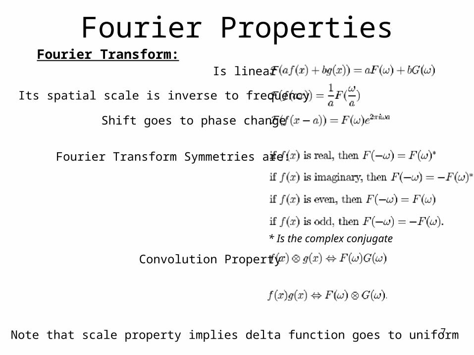
Fourier PropertiesFourier Transform:
Is linear
Its spatial scale is inverse to frequency
Shift goes to phase change
Fourier Transform Symmetries are:
Convolution Property
Note that scale property implies delta function goes to uniform
* Is the complex conjugate

8
Animals and Machines live in a discrete world. To move the continuous Fourier world to its discrete version, we sample• => Multiply by infinite series of delta functions spaced apart• => Convolve with a uniform function inversely spaced
Fourier Discrete (DFT)
/1

9
Fourier Discrete (DFT) 2All real world signals are “band limited” That is, they don’t have infinite frequenciesnor infinite spatial extend. This is good, otherwise our discrete Fourier copies wouldcollide and alias together. But, what if we still sample too seldom? Even band limitedwill eventually collide.
How do we keep the copiesapart? Sample at at least twice the signal’s band limitfrequency => Niquist Criterion
interval. sampleour is where2
1
c

10
2D DFTDiscrete Fourier Transform (DFT)
Inverse DFT
Optimally implemented on serial machines via the “Fast Fourier Transform” (FFT), DFT is faster on parallel machines.
11
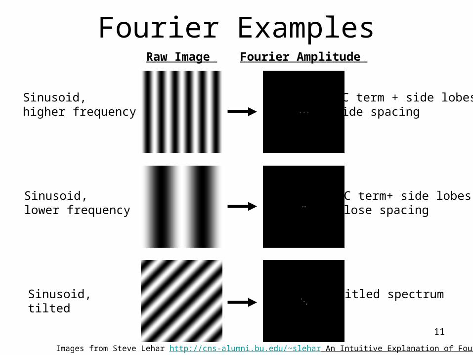
Fourier ExamplesRaw Image Fourier Amplitude
Sinusoid,higher frequency
Sinusoid,lower frequency
Sinusoid,tilted
DC term + side lobeswide spacing
DC term+ side lobesclose spacing
Titled spectrum
Images from Steve Lehar http://cns-alumni.bu.edu/~slehar An Intuitive Explanation of Fourier Theory
12
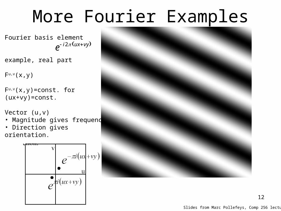
Fourier basis element
example, real part
Fu,v(x,y)
Fu,v(x,y)=const. for (ux+vy)=const.
Vector (u,v)• Magnitude gives frequency• Direction gives orientation.
e i2 uxvy
Slides from Marc Pollefeys, Comp 256 lecture 7
More Fourier Examples

13
Here u and v are larger than in the previous slide.
Slides from Marc Pollefeys, Comp 256 lecture 7
More Fourier Examples

14
And larger still...
Slides from Marc Pollefeys, Comp 256 lecture 7
More Fourier Examples
15
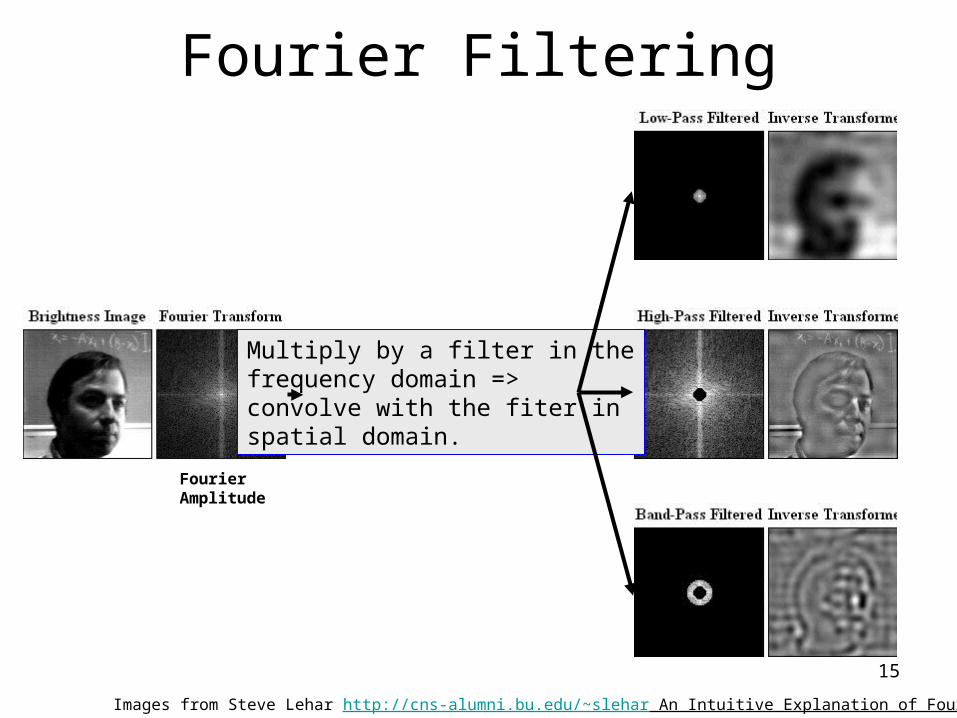
Fourier Filtering
Images from Steve Lehar http://cns-alumni.bu.edu/~slehar An Intuitive Explanation of Fourier Theory
FourierAmplitude
Multiply by a filter in thefrequency domain => convolve with the fiter inspatial domain.

16
Fourier LensRemember that Fourier transform takes delta functions to uniform, and uniform to delta?
Figures from Steve Lehar http://cns-alumni.bu.edu/~slehar An Intuitive Explanation of Fourier Theory
Well, when focused at infinity (parallel rays to a point), so do lenses!
A lens approximates a Fourier transform processed at the speed of light

17
Phase Caries More Information
MagnitudeandPhase:
RawImages:
Reconstruct(inverse FFT)mixing themagnitude andphase images
Phase “Wins”

18
Phase Coherence for Feature Detection?
Images: Peter Kovesi, Proc. VIIth Digital Image Computing: Techniques and Applications, Sun C., Talbot H., Ourselin S. and Adriaansen T. (Eds.), 10-12 Dec. 2003, Sydney
Note that the Fourier components for a square wave cohere (are in phase) at the step junction Here, they must all pass through zero right at the step edge, and achieve local maximums at the “corners”.
Phase coherence is maximal at “corner points” of triangle and trapezoid waves too
Triangle Wave Trapezoid Wave

19
Morrone defined a measure that at absolute phase coherence will be 1 – everythingpoints in the same direction -- and for no phase coherence will be zero. Local maximumsindicate edges and corners, insensitive to contrast in the image.
In practice, these local components are calculated with Gabor filters at severalorientations that can yield oriented edges and corners.
Phase Coherence for Feature DetectionGist of the idea: Fourier transform yields a series of real and imaginary sinusoidal terms.At any point x, the local Fourier components will each have an amplitude An(x) and a phase angle φn(x). Vector addition of these terms yields an vector E(x) at the average phase angle.
Images: Peter Kovesi, Proc. VIIth Digital Image Computing: Techniques and Applications, Sun C., Talbot H., Ourselin S. and Adriaansen T. (Eds.), 10-12 Dec. 2003, Sydney

20
Phase Coherence for Feature Detection
Images: Peter Kovesi, Proc. VIIth Digital Image Computing: Techniques and Applications, Sun C., Talbot H., Ourselin S. and Adriaansen T. (Eds.), 10-12 Dec. 2003, Sydney
Comparison of phase vs. Harris Corner detector. Harris response varies by 2 or moreorders of magnitude…threshold? Phase can only vary between 0 and 1 and isnot sensitive to contrast or lighting.

21
Gabor filters and JetsGlobal information is used for physical systems
identification.– Impulse response of a centrifuge to identify resonance
points which indicate which spin frequencies to avoid.
Local information is used for physical signal analysis. – In images, it is the relationship of details that matter, not
(usually) things like average brightness.
In 1946, Gabor suggested representing signals over space and time called Information diagrams. He showed that a Gaussian occupies minimal area in such diagrams. Time and Frequency analysis are the two extremes of such an analysis.
22
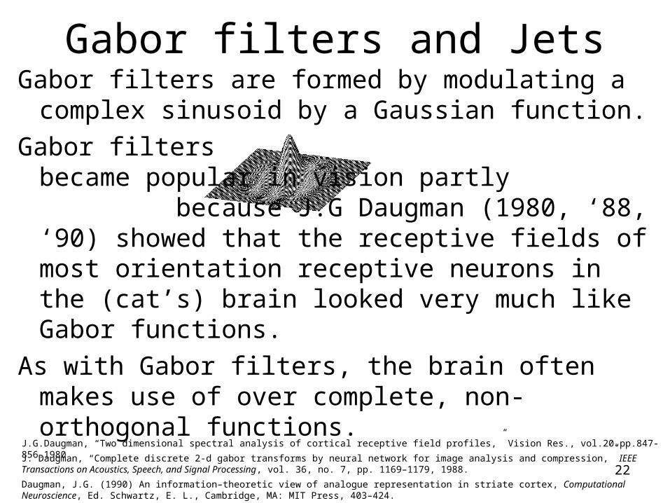
Gabor filters are formed by modulating a complex sinusoid by a Gaussian function.
Gabor filters became popular in vision partly because J.G Daugman (1980, ‘88, ‘90) showed that the receptive fields of most orientation receptive neurons in the (cat’s) brain looked very much like Gabor functions.
As with Gabor filters, the brain often makes use of over complete, non-orthogonal functions.
Gabor filters and Jets
Daugman, J.G. (1990) An information–theoretic view of analogue representation in striate cortex, Computational Neuroscience, Ed. Schwartz, E. L., Cambridge, MA: MIT Press, 403–424.
J. Daugman, “Complete discrete 2-d gabor transforms by neural network for image analysis and compression,” IEEE Transactions on Acoustics, Speech, and Signal Processing, vol. 36, no. 7, pp. 1169–1179, 1988.
J.G.Daugman, “Two dimensional spectral analysis of cortical receptive field profiles,” Vision Res., vol.20.pp.847-856.1980

23
Gabor filters and Jets
2D Gabor filter:
Rotated Gaussian
Oriented ComplexSinusoid
sinusoid. theoffrequency radial theis andfilter theofn orientatio
theis filter, theofextent spatial thecontrol and where 2x
2x
W
Depending on one’s task (object ID, texture analysis, tracking,…) one must then decide what size filters, in what orientations and what frequencies to use.

24
Gabor filters and Jets
In practice, once the scales, orientation and radial frequencies are chosen one usually sets up filters in quadrature (90o phase shift) pairs and just empirically normalizes them such that the response is zero to a uniform background.
Quadrature pairs, in practice the center point (p,q) is set to (0,0).
The magnitude response is then calculated as:

25
Gabor filters and JetsVon Der Malsburg organized Gabor filters at multiple scales and orientationsin a vector, or “Jet”
A graph of such Jets (“Elastic Graph Matching”) has proven to be a good “primitive” for object recognition.
Image from Laurenz Wiskott, http://itb.biologie.hu-berlin.de/~wiskott/
L. Wiskott, J-M. Fellous, N. Kuiger, C. Malsburg, “Face Recognition by Elastic Bunch Graph Matching”, IEEE Transactions on Pattern Analysis and Machine Intelligence, vol.19(7), July 1997, pp. 775-779.

26
Gabor filters and Jets Example
Gang Song, Tao Wang, Yimin Zhang, Wei Hu, Guangyou Xu, Gary Bradski, “Face Modeling and Recognition Using Bayesian Networks”, Submitted to CVPR 2004
Gabor Filters used
BayesNet Facial Model Instead of anMalsburg Elastic Graph Model (EGM).
Pose
Pose variable added
Training and Recognition Flow Chart
Results: BN Pose Face Rec. vs. EGM

27
Scale• 3D to 2D Perspective projections give widely
varying scale for the same object. Computer vision needs to address scale.
• Gabor discussion above addressed image scale via the sigma of the modulating Gaussians and the frequency of the complex sinusoid.
• We can directly deal with scale by repeatedly down-sampling the image to look for courser and courser patterns. We call this scale space, or Image Pyramids

28
Image Pyramids
Gaussianblur
GaussianPyramid
LaplacianPyramid
Commonly, wedown-sampleby 2 or sqrt(2).Sqrt(2) obviouslycalls for inter-pixelinterpolation
Laplacian Pyramid~ “Error Pyramid
For down-sample by2, typical Gaussiansigma is 1.4. For Sqrt(2) sigma istypically the sqrt(1.4).
Full power 2 pyramidonly doubles the numberof pixels to process.

29
SteerabilityBill Freeman, in his 1992 Thesis determined the necessary conditions for “Steerability”-- the ability to synthesize a filter of any orientation from a linear combination of filters at fixed orientations.
The simplest example of this is oriented first derivative of Gaussian filters, at 0o and 90o:
Steering Eqn:
Filter Set:0o 90o Synthesized 30o
Response:
Raw Image
Taken from:W. Freeman, T. Adelson, “The Design and Use of Sterrable Filters”, IEEE Trans. Patt, Anal. and Machine Intell., vol 13, #9, pp 891-900, Sept 1991

30
SteerabilityFreeman showed that any band limited signal could form a steerable basis with as manybases as it had non-zero Fourier coefs.
Important example is 2nd derivative of Gaussian (~Laplacian):
Taken from: W. Freeman, T. Adelson, “The Design and Use of Steerable Filters”, IEEE Trans. Patt, Anal. and Machine Intell., vol 13, #9, pp 891-900, Sept 1991

31
Steerable PyramidWe may combine Steerability with Pyramids to get a Steerable Laplacian Pyramid as shown below
Images from: http://www.cis.upenn.edu/~eero/steerpyr.html
High pass, sinceband pass in pyramidlow pass at bottom.
Low Pass
Orie
nted
Decomposition Reconstruction
2 Level decompositionof white circle example:

32
Scale Invariant Feature Transform
• Idea is to find local features that stay the same (as much as possible) under:– Scale change– 2D rotation in the image x,y plane– 3D rotation (affine variation)– Illumination
• Collections of such features can be used for reliable– 3D object recognition– User interface, toy interface– Robot localization, navigation and mapping– Digital image stitching, organization– 3D scene understanding

33
Scale Invariant Feature Transform
High Level Algorithm1. Find peak responses (over scale) in
Laplacian pyramid.
2. Find response with sub-pixel accuracy.
3. Only keep “corner like” responses
4. Assign orientation
5. Create recognition signature
6. Solve affine parameters (~3D rot. changes)

34
Scale Invariant Feature TransformFrom Gaussian scale pyramid -- create Difference of Gaussian (DOG) images
And find maximum response over space and scale:
Images from: David G. Lowe, Object recognition from local scale-invariant features, International Conference on Computer Vision, Corfu, Greece (September 1999), pp. 1150-1157

35
Scale Invariant Feature TransformAt the location and scale of peak found, find the gradient orientation:
Use the gradients to only keep “corner like” peaks in manner similar to Harris corner detector:
At each peak location and scale, use gradients to form slip tolerant orientation histogram recognition keys:
Imag
es fr
om: D
avid
G. L
owe,
Ob
ject
rec
og
nit
ion
fro
m lo
cal s
cale
-in
vari
ant
feat
ure
s,
Inte
rnat
iona
l Con
fere
nce
on C
ompu
ter
Vis
ion,
Cor
fu, G
reec
e (S
epte
mbe
r 19
99),
pp.
115
0-11
57

36
Scale Invariant Feature TransformTo account for out of image plane (3D) rotation, solve for affine distortion parameters:
Eqns from: David G. Lowe, Object recognition from local scale-invariant features, International Conference on Computer Vision, Corfu, Greece (September 1999), pp. 1150-1157
For features found, set up system of equations
Which take the form of . Over determined (least sqrs) solution is then:

37
Scale Invariant Feature TransformRecognition example. Learned models of SIFT features, and got object outline frombackground subtraction:
Objects may then be found under occlusion and 3D rotation:
Imag
es fr
om: D
avid
Low
e, O
bje
ct R
eco
gn
itio
n f
rom
Lo
cal S
cale
-In
vari
ant
Fea
ture
s P
roc.
of
the
Inte
rnat
iona
l Con
fere
nce
on C
ompu
ter
Vis
ion,
Cor
fu (
Sep
t. 19
99)
38
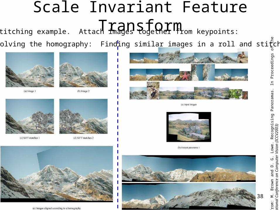
Scale Invariant Feature TransformImage stitching example. Attach images together from keypoints:
Solving the homography: Finding similar images in a roll and stitching:
Imag
es fr
om: M
. Bro
wn
and
D. G
. Low
e. R
ecog
nisi
ng P
anor
amas
. In
Pro
ceed
ings
of t
he
9th
Inte
rnat
iona
l Con
fere
nce
on C
ompu
ter
Vis
ion
(IC
CV
2003
)

39
Scale Invariant Feature TransformLocalizing Example:
Given key images, find and trigger on them1: Find different views of same scene in video2:
2) Josef Sivic and Andrew Zisserman, Video Google: A Text Retrieval Approach to Object Matching in Videos, ICCV 2003
1) David G. Lowe, Distinctive Image Features from Scale-Invariant Keypoints, Submitted to International Journal of Computer Vision. Version date: June 2003

40
Log-Polar TransformGo from Euclidian (x,y) to log-polar space log(rei) => (log r, ) space. Log-polartransform is always done relative to a chosen center point (xc,yc):
(xc,yc)
r
x
y
log rLog-Polar
r(xc,yc)
x
y
Log-Polarlog r
Rotation and scale are converted to shifts along the or log r axis. Shifting back to a canonical location gives rotation and scale invariance. If used on a Fourier image (translation invariant), we getrotation, scale and translation invariance (called Fourier-Mellin transform)1. 1)
Imag
es, f
urth
er a
dvan
ces
in: G
eorg
e W
olbe
rg, S
iava
sh Z
okai
, RO
BU
ST
IM
AG
E R
EG
IST
RA
TIO
N U
SIN
G L
OG
-PO
LA
R T
RA
NS
FO
RM
, IC
IP 2
000

41
Bilateral FilteringWe want smoothing that preserves edges.
Typically done via P. Perona and J. Malik anisotropic diffusion. More clever is the Tomasi and Manduchi* approximation:
• Rather than just convolve with a Gaussian in space• the convolution weights use a Gaussian in space together with a
Gaussian in gray level values.
* C. Tomasi and R. Manduchi, "Bilateral Filtering for Gray and Color Images", Proceedings of the 1998 IEEE International Conference on Computer Vision, Bombay, India
=

42
But Bio-Vision is more dynamic• Artifacts of competitive edge/diffusion process:
Neon Color Spreading Illusion
Best explanation is Grossberg and Mingolla – edge detectors need to be “shut off”, performed by competitive inhibition. When weaker edges meet stronger, the weaker edge is suppressed breaking the dikes that hold back the diffusion process. When the edges are disconnected, the illusion goes away or is diminished below:
Grossberg, S., & Mingolla, E. (1985). Neural Dynamics of Form Perception: Boundary Completion. Psychol. Rev., 92, 173--211.
43
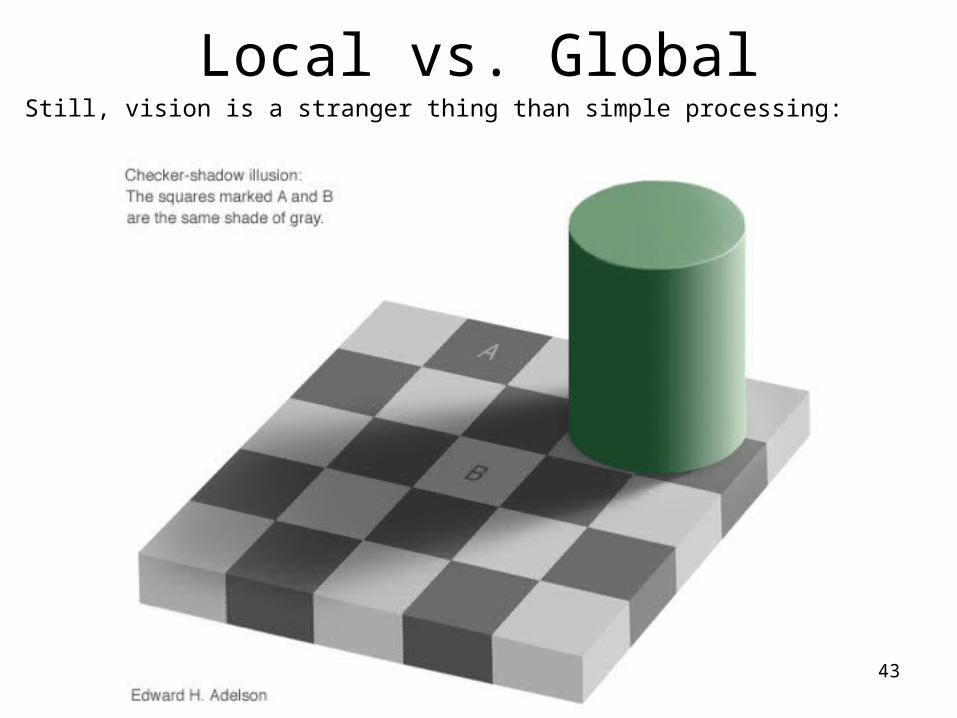
Local vs. GlobalStill, vision is a stranger thing than simple processing:
44
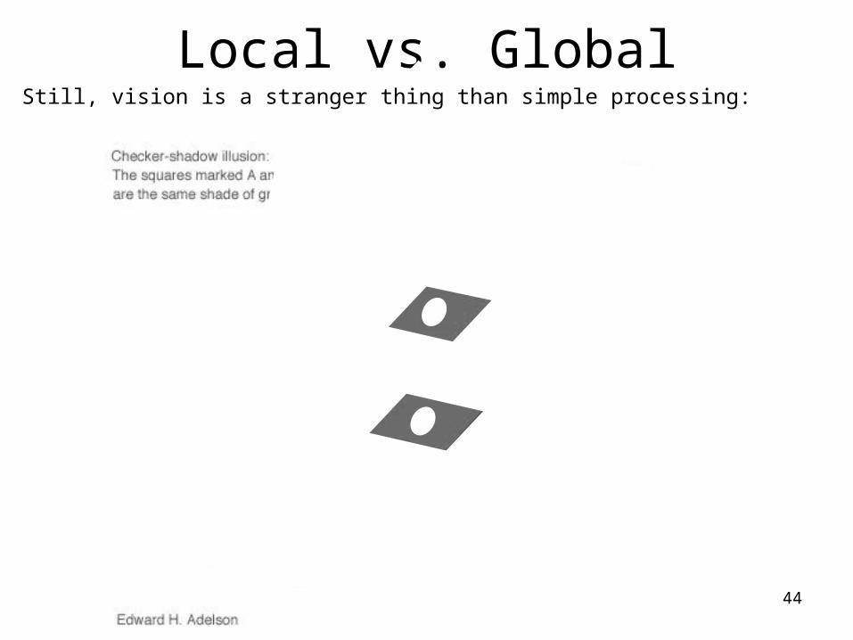
Local vs. GlobalStill, vision is a stranger thing than simple processing:

45
Computer vision often misses the fact that vision is an active sense
These lines are straight Nothing is moving here


