84
1 Data Mining and Knowledge Acquisition — Chapter 6 — BIS 541 2013/2014 Summer
| Date post: | 27-Dec-2015 |
| Category: |
Documents |
| Upload: | paula-preston |
| View: | 215 times |
| Download: | 1 times |

1
Data Mining and Knowledge Acquisition
— Chapter 6 —
BIS 541
2013/2014 Summer

2
Chapter 5: Mining Association Rules in Large Databases
Association rule mining Mining single-dimensional Boolean association
rules from transactional databases Mining multilevel association rules from
transactional databases Mining multidimensional association rules from
transactional databases and data warehouse From association mining to correlation analysis Constraint-based association mining Summary
3
What Is Association Mining?
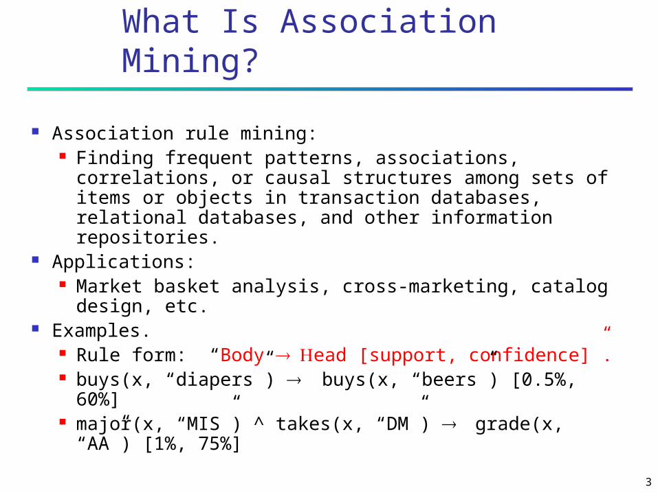
Association rule mining: Finding frequent patterns, associations,
correlations, or causal structures among sets of items or objects in transaction databases, relational databases, and other information repositories.
Applications: Market basket analysis, cross-marketing, catalog
design, etc. Examples.
Rule form: “Body ead [support, confidence]”. buys(x, “diapers”) buys(x, “beers”) [0.5%, 60%] major(x, “MIS”) ^ takes(x, “DM”) grade(x, “AA”)
[1%, 75%]

4
Association Rule: Basic Concepts
Given: (1) database of transactions, (2) each transaction is a list of items (purchased
by a customer in a visit) Find: all rules that correlate the presence of one set
of items with that of another set of items E.g., 98% of people who purchase tires and auto
accessories also get automotive services done The user specifies
Minimum support level Minimum confidence level Rules exceeding the two trasholds are listed as
interesting

5
Basic Concepts cont.
I:{i1,..,im} set of all items, T any transaction AT: T contains the itemset A AT, BT A,B itemsets Examine rule like: AB where AB=,
support s: P(AB) frequency of transactions containing both A
and B confidence c: P(BA) = P(AB)/P(A)
Conditional probability that a transaction containing A contains B

6
Rule Measures: Support and Confidence
Find all the rules X & Y Z with minimum confidence and support
support, s, probability that a transaction contains {X Y Z}
confidence, c, conditional probability that a transaction having {X Y} also contains Z
Transaction ID Items Bought2000 A,B,C1000 A,C4000 A,D5000 B,E,F
Let minimum support 50%, and minimum confidence 50%, we have
A C (50%, 66.6%) C A (50%, 100%)
Customerbuys diaper
Customerbuys both
Customerbuys beer

7
Frequent itemsets
Strong association rules: Support rule > min_support Confidence rule > min_confidence
k-item set: itemsets containing k items occurrence frequency=count=support count: Minimum support count = min_sup*#transactions in database frequent item sets:
İtemsets satisfying minimum support count The Apriori Algorithm has two steps:
(1) - Find all frequent itemsets (2) - Genertate strong association rules from
frequent itemsets
8
Mining Association Rules—An Example(1)
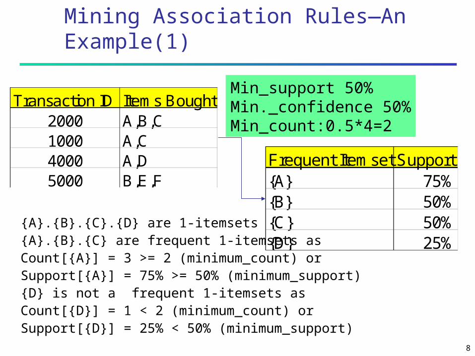
{A}.{B}.{C}.{D} are 1-itemsets{A}.{B}.{C} are frequent 1-itemsets asCount[{A}] = 3 >= 2 (minimum_count) orSupport[{A}] = 75% >= 50% (minimum_support){D} is not a frequent 1-itemsets asCount[{D}] = 1 < 2 (minimum_count) orSupport[{D}] = 25% < 50% (minimum_support)
Transaction ID Items Bought2000 A,B,C1000 A,C4000 A,D5000 B,E,F
Frequent Itemset Support{A} 75%{B} 50%{C} 50%{D} 25%
Min_support 50%Min._confidence 50%Min_count:0.5*4=2

9
Mining Association Rules—An Example(2)
{A.B}.{A.C}.{A.D}.{B.C} are 2-itemsets{A.C}is frequent 2-itemsets asCount[{A.C}] = 2 >= 2 (minimum_count) orSupport[{A.C}] = 50% >= 50% (minimum_support){A.B}.{A.D} are not frequent 2-itemsets asCount[{A.D}] = 1 < 2 (minimum_count) orSupport[{A.D}] = 25% < 50% (minimum_support)
Transaction ID Items Bought2000 A,B,C1000 A,C4000 A,D5000 B,E,F
Frequent Itemset Support{A.B} 25%{A.C} 50%{A.D} 25%{B,C} 25%
Min_support 50%Min._confidence 50%Min_count:0.5*4=2

10
Mining Association Rules—An Example(3)
For rule A C:support = support({A C}) = 50%confidence = support({A C})/support({A}) =
66.6%Strong rule as support >=min_support confidence >= min_confidence
Transaction ID Items Bought2000 A,B,C1000 A,C4000 A,D5000 B,E,F
Frequent Itemset Support{A} 75%{B} 50%{C} 50%{A,C} 50%
Min. support 50%Min. confidence 50%

11
The Apriori Principle
The Apriori principle:Any subset of a frequent itemset must be
frequent{A.C} is a frequent 2-itemset{A} and {C}: subsets of {A,C} must be frequent
1-itemsets
Transaction ID Items Bought2000 A,B,C1000 A,C4000 A,D5000 B,E,F
Frequent Itemset Support{A} 75%{B} 50%{C} 50%{A,C} 50%
Min. support 50%Min. confidence 50%
12
Apriori Algorithme has two steps
(1)-Find the frequent itemsets: the sets of items that have minimum support (the key step)
A subset of a frequent itemset must also be a frequent itemset
i.e., if {AB} is a frequent itemset, both {A} and {B} should be a frequent itemsets
Iteratively find frequent itemsets with cardinality from 1 to k (k-itemset)
Until k is an empty set
(2)-Use the frequent itemsets to generate association rules.

13
Generation of frequent itemsets from candidate itemsets (Step 1)
C1L1 C2L2 C3 L3 C4L4… From Ck (candidate k-itemsets) generate Lk :Ck Lk
From candidate k itemsets generate frequent k itemsets
(a)-Using the Apriori principle that: Eliminate itemset sk in Ck if
At least one k-1 subset of sk is not in Lk-1
(b)-For candidate k itemsets in Ck
Make a database scan to eliminate those itemsets whose support counts are below the critical min support cout
From frequent k itemsets Lk generate candidate k+1 itemsets Ck+1 : Lk Ck+1
Self joining any Lk with Lk

14
Self Join operation
Sort the items in any li Lk in some lexicographic order li[1]<li[2]<,… <li[k-1]<li[k]
li and lj are elements of Lk li.lj Lk
If li[1]=lj[1] and li[2]=lj[2] and … li[k-1]=lj[k-1] and li[k]<lj[k]
The first k-1 elements are the same Only the last elements are different
li lj satisfiing the above condition Construct the item set lk+1:
li[1], li[2],… li[k-1],li[k], lj[k] common items the k-1 items are taken form li or lj k th item is taken from li k+1 th item is from lj

15
Example of Self Join operation Lexigographic order: alphabetic a<b<c<d....
L3={abc, abd, acd, ace, bcd}
Self-joining: L3*L3 Step(2)
abcd from abc and abd
acde from acd and ace
Pruning by Apriori principle: Step(1a)
acde is removed because ade is not in L3
C4={abcd}

16
The Apriori Algorithm — Examplemin support cont=2
TID Items100 1 3 4200 2 3 5300 1 2 3 5400 2 5
Database D itemset sup.{1} 2{2} 3{3} 3{4} 1{5} 3
itemset sup.{1} 2{2} 3{3} 3{5} 3
Scan D
C1L1
itemset{1 2}{1 3}{1 5}{2 3}{2 5}{3 5}
itemset sup{1 2} 1{1 3} 2{1 5} 1{2 3} 2{2 5} 3{3 5} 2
itemset sup{1 3} 2{2 3} 2{2 5} 3{3 5} 2
L2
C2 C2
Scan D
C3 L3itemset{2 3 5}
Scan D itemset sup{2 3 5} 2

17
Example 6.1 Han
TID_____list of item_Ids T1001 2 5 9 transactions T2002 4 D=9 T300 2 3 minimum transaction T4001 2 4 support_count=2 T5001 3 min_sup=2/9=22% T6002 3 T7001 3 min conf: 70% T8001 2 3 5 T9001 2 3
Find strong association rules: having min sup count of 2 and min confidence %70

18
Data Dictionary
1: milk 2: apple 3: butter 4: bread 5: orange

19
1th iteration of algorithm
C1: itemset sup_count L1:itemset sup_count 1 6 1 6 2 7 2 7 3 6 3 6 4 2 4 2 5 2 5 2
C2:L1 join L1, itemset sup_count L2 itset supcount
1 2 4 1 2 4 1 3 4 1 3 4 1 4 1x 1 5 2 1 5 2 2 3 4 2 3 4 2 4 2 2 4 2 2 5 2 2 5 2 frequent 2 item sets L2
3 4 0x those itemsets in C2
3 5 1x having minimum support 4 5 0x Step (1b)

20
3 th iteration
Self join to get C3 Step (2) C3: L2 join L2: [1 2 3], [1 2 5],[1 3 5],[2 3 4], [2 3 5],[2 4 5] Now Step (1a) Apply Apriori to every itemset in C3
2 item subsets of [1 2 3]:[1 2],[1 3],[2 3] all 2 items sets are members of L2
keep [1 2 3] in C3
2 item subsets of [1 2 5]:[1 2],[1 5],[2 5] all 2 items sets are members of L2
keep [1 2 5] in C3
2 item subsets of [1 3 5]:[1 3],[1 5],[3 5] [3 5] is not a members of L2 so it si not frequent remove [1 2 5] from C3

21
3 iteration cont.
2 item subsets of [2 3 4]:[2 3],[2 4],[3 4] [3 4] is not a members of L2 so it si not frequent remove [2 3 4] from C3
2 item subsets of [2 3 5]:[2 3],[2 5],[3 5] [3 5] is not a members of L2 so it si not frequent remove [2 3 5] from C3
2 item subsets of [2 4 5]:[2 4],[2 5],[4 5] [4 5] is not a members of L2 so it si not frequent remove [2 4 5] from C3
C3:[1 2 3],[1 2 5] after pruning

22
4 th iteration
C3L3 check min support Step (1b) L3:those item sets having minimum support L3: item sets minsupcount
1 2 3 2 1 2 5 2
L3 join L3 to generate C4 Step (2) L3 join L3: 1 2 3 5 pruned since its subset [2 3 5] is not frequent C4= the algorithm terminates

23
Generating Association Rules from frequent itemsets
Strong rules min support and min confidence
confidence(AB)= P(BA):sup_count(AB) sup_count(A) for each frequent itemset l
generate non empty subsets of l: denoted by s
For each sl construct rules: s (l-s) Satısfying the condition:
sup_count(l)/sup_count(s)>=min_conf are listed as interestıng

24
Example 6.2 Han cont.
the 3-frequent item set l:[1 2 5]: transaction containing milk, apple and orange is frequent
non empty subsets of l are [1 2],[1 5],[2 5],[1],[2],[5]
the resulting association rules are: 125 conf: 2/4=50% 152 conf: 2/2=100% 251 conf: 2/2=100% 125 conf: 2/6=33% 215 conf: 2/7=29% 512 conf: 2/2=100%
if min conf: 70% 2th 3th and last rules are strong

25
Example 6.2 cont. Detail on confidence for two rules
For the rule 152 conf: s(1,2,5)/s(1,5) conf: 2/2=100% >= 70% A strong rule
For the rule 215 conf: s(1,2,5)/s(2) conf: 2/7=29% < 70% Not a strong rule

26
Exercise
Find all strong association rules in Example 6.2 Check minimum confindence for 2-frequent intemsets
[1,2], [1,3], [1,5], [2,3], [2,4], [2,5] 12, 21 25, 52 exetra
for 3-frequent intemset [1,2,5] 123 3 12 exetra

27
Exercise
a) Suppose A B and B C are strong rules Dose this imply that A C is also a strong
rule? b) Suppose A B and A C are strong rules Dose this imply that B C is also a strong
rule? c) Suppose A C and B C are strong rules Dose this imply that A and B C is also a
strong rule?

28
Bottleneck of Frequent-pattern Mining
Multiple database scans are costly Mining long patterns needs many passes of
scanning and generates lots of candidates To find frequent itemset i1i2…i100
# of scans: 100 # of Candidates: (100
1) + (1002) + … + (1
10
00
0) =
2100-1 = 1.27*1030 !
Bottleneck: candidate-generation-and-test Can we avoid candidate generation?
29
Is Apriori Fast Enough? — Performance Bottlenecks
The core of the Apriori algorithm: Use frequent (k – 1)-itemsets to generate candidate frequent
k-itemsets Use database scan and pattern matching to collect counts
for the candidate itemsets The bottleneck of Apriori: candidate generation
Huge candidate sets: 104 frequent 1-itemset will generate 107 candidate 2-
itemsets To discover a frequent pattern of size 100, e.g., {a1, a2,
…, a100}, one needs to generate 2100 1030 candidates.
Multiple scans of database: Needs (n +1 ) scans, n is the length of the longest
pattern

30
Mining Frequent Patterns Without Candidate Generation
Compress a large database into a compact, Frequent-Pattern tree (FP-tree) structure
highly condensed, but complete for frequent pattern mining
avoid costly database scans Develop an efficient, FP-tree-based frequent
pattern mining method A divide-and-conquer methodology: decompose
mining tasks into smaller ones Avoid candidate generation: sub-database test
only!

31
Construct FP-tree from a Transaction DB
{}
f:4 c:1
b:1
p:1
b:1c:3
a:3
b:1m:2
p:2 m:1
Header Table
Item frequency head f 4c 4a 3b 3m 3p 3
min_support = 0.5
TID Items bought (ordered) frequent items100 {f, a, c, d, g, i, m, p} {f, c, a, m, p}200 {a, b, c, f, l, m, o} {f, c, a, b, m}300 {b, f, h, j, o} {f, b}400 {b, c, k, s, p} {c, b, p}500 {a, f, c, e, l, p, m, n} {f, c, a, m, p}
Steps:
1. Scan DB once, find frequent 1-itemset (single item pattern)
2. Order frequent items in frequency descending order
3. Scan DB again, construct FP-tree

32
Benefits of the FP-tree Structure
Completeness: never breaks a long pattern of any transaction preserves complete information for frequent
pattern mining Compactness
reduce irrelevant information—infrequent items are gone
frequency descending ordering: more frequent items are more likely to be shared
never be larger than the original database (if not count node-links and counts)
Example: For Connect-4 DB, compression ratio could be over 100

33
Chapter 5: Mining Association Rules in Large Databases
Association rule mining Mining single-dimensional Boolean association
rules from transactional databases Mining multilevel association rules from
transactional databases Mining multidimensional association rules from
transactional databases and data warehouse From association mining to correlation analysis Constraint-based association mining Summary

34
Multiple-Level Association Rules
Items often form hierarchy. Items at the lower level are
expected to have lower support.
Rules regarding itemsets at
appropriate levels could be quite useful.
Transaction database can be encoded based on dimensions and levels
We can explore shared multi-level mining
Food
breadmilk
skim
SunsetFraser
2% whitewheat
TID ItemsT1 {111, 121, 211, 221}T2 {111, 211, 222, 323}T3 {112, 122, 221, 411}T4 {111, 121}T5 {111, 122, 211, 221, 413}

35
Mining Multi-Level Associations
A top_down, progressive deepening approach: First find high-level strong rules:
milk bread [20%, 60%]. Then find their lower-level “weaker” rules:
2% milk wheat bread [6%, 50%]. Variations at mining multiple-level association
rules. Level-crossed association rules:
2% milk Wonder wheat bread Association rules with multiple, alternative
hierarchies: 2% milk Wonder bread
36
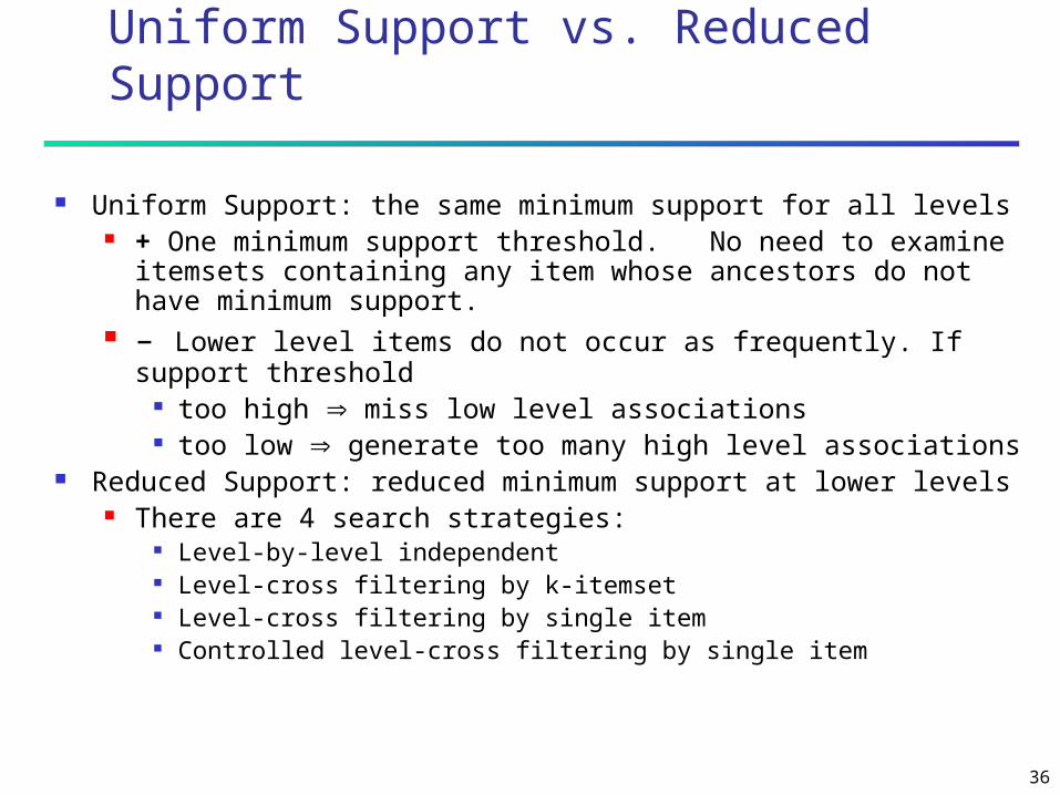
Multi-level Association: Uniform Support vs. Reduced Support
Uniform Support: the same minimum support for all levels + One minimum support threshold. No need to examine
itemsets containing any item whose ancestors do not have minimum support.
– Lower level items do not occur as frequently. If support threshold
too high miss low level associations too low generate too many high level associations
Reduced Support: reduced minimum support at lower levels There are 4 search strategies:
Level-by-level independent Level-cross filtering by k-itemset Level-cross filtering by single item Controlled level-cross filtering by single item

37
Uniform Support
Multi-level mining with uniform support
Milk
[support = 10%]
2% Milk
[support = 6%]
Skim Milk
[support = 4%]
Level 1min_sup = 5%
Level 2min_sup = 5%
Back

38
Reduced Support
Multi-level mining with reduced support
2% Milk
[support = 6%]
Skim Milk
[support = 4%]
Level 1min_sup = 5%
Level 2min_sup = 3%
Back
Milk
[support = 10%]

39
Controlled level-cross filtering by single item Specify a level passage treshold for each
level k min_sup_T(k+1)<LPT(k)<min_sup_T(k) Example:
High level milk min supp=5%
Low level 2% milk,skim milk Min supp = 3%
Level passage trashold = 4%

40
Multi-level Association: Redundancy Filtering
Some rules may be redundant due to “ancestor” relationships between items.
Example milk wheat bread [support = 8%, confidence =
70%] 2% milk wheat bread [support = 2%, confidence =
72%] We say the first rule is an ancestor of the second
rule. A rule is redundant if its support is close to the
“expected” value, based on the rule’s ancestor.

41
Multi-Level Mining: Progressive Deepening
A top-down, progressive deepening approach: First mine high-level frequent items:
milk (15%), bread (10%) Then mine their lower-level “weaker” frequent
itemsets: 2% milk (5%), wheat bread (4%) Different min_support threshold across multi-
levels lead to different algorithms: If adopting the same min_support across multi-
levelsthen toss t if any of t’s ancestors is infrequent.
If adopting reduced min_support at lower levelsthen examine only those descendents whose
ancestor’s support is frequent/non-negligible.
42
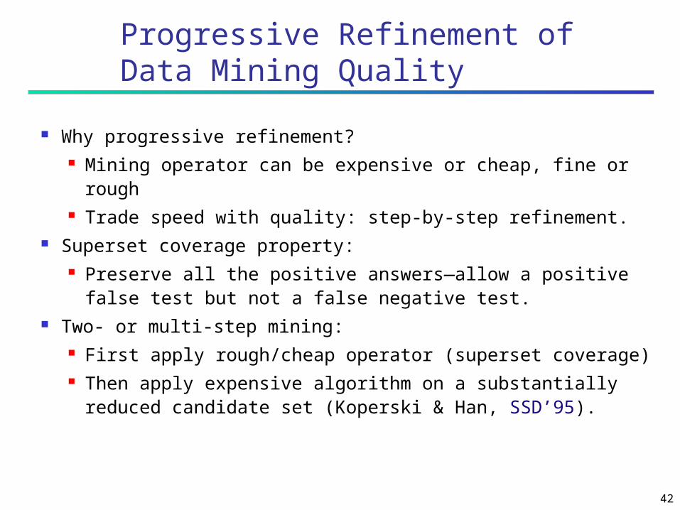
Progressive Refinement of Data Mining Quality
Why progressive refinement? Mining operator can be expensive or cheap, fine or
rough Trade speed with quality: step-by-step refinement.
Superset coverage property: Preserve all the positive answers—allow a positive
false test but not a false negative test. Two- or multi-step mining:
First apply rough/cheap operator (superset coverage)
Then apply expensive algorithm on a substantially reduced candidate set (Koperski & Han, SSD’95).

43
Chapter 5: Mining Association Rules in Large Databases
Association rule mining Mining single-dimensional Boolean association
rules from transactional databases Mining multilevel association rules from
transactional databases Mining multidimensional association rules from
transactional databases and data warehouse From association mining to correlation analysis Constraint-based association mining Summary

44
Interestingness Measurements
Objective measuresTwo popular measurements: support; and confidence
Subjective measures (Silberschatz & Tuzhilin, KDD95)A rule (pattern) is interesting if it is unexpected (surprising to the user);
and/or actionable (the user can do something with
it)
45
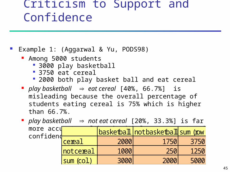
Criticism to Support and Confidence
Example 1: (Aggarwal & Yu, PODS98) Among 5000 students
3000 play basketball 3750 eat cereal 2000 both play basket ball and eat cereal
play basketball eat cereal [40%, 66.7%] is misleading because the overall percentage of students eating cereal is 75% which is higher than 66.7%.
play basketball not eat cereal [20%, 33.3%] is far more accurate, although with lower support and confidence
basketball not basketball sum(row)cereal 2000 1750 3750not cereal 1000 250 1250sum(col.) 3000 2000 5000
46
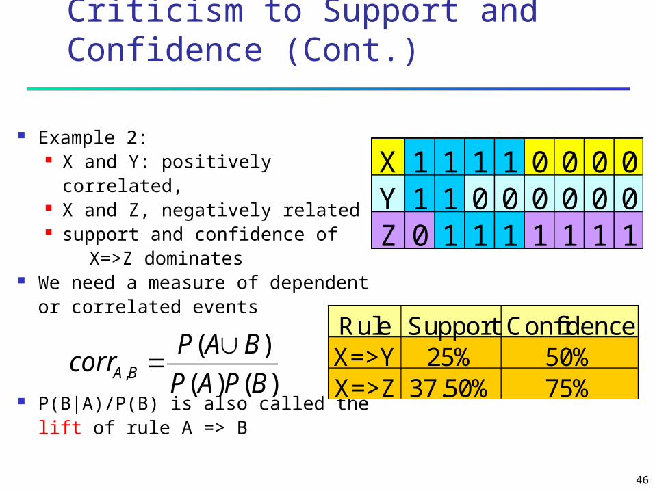
Criticism to Support and Confidence (Cont.)
Example 2: X and Y: positively
correlated, X and Z, negatively related support and confidence of X=>Z dominates
We need a measure of dependent or correlated events
P(B|A)/P(B) is also called the lift of rule A => B
X 1 1 1 1 0 0 0 0Y 1 1 0 0 0 0 0 0Z 0 1 1 1 1 1 1 1
Rule Support ConfidenceX=>Y 25% 50%X=>Z 37.50% 75%)()(
)(, BPAP
BAPcorr BA

47
Other Interestingness Measures: Interest Interest (correlation, lift)
taking both P(A) and P(B) in consideration
P(A^B)=P(B)*P(A), if A and B are independent
events
A and B negatively correlated, if the value is less
than 1; otherwise A and B positively correlated
)()(
)(
BPAP
BAP
X 1 1 1 1 0 0 0 0Y 1 1 0 0 0 0 0 0Z 0 1 1 1 1 1 1 1
Itemset Support InterestX,Y 25% 2X,Z 37.50% 0.9Y,Z 12.50% 0.57

48
Example
Total transactions 10,000 İtems C:computers, V: video V: 7,500 C: 6,000 C and V: 4,000
Min_support: 0.3 min_conf:0,50 Consider the rule: Buy(X: computer) buy(X: video)
Support : = 4000/10000 = 0.4 Confidence: P(C and V) /P(C) = 4000/6000 =%66 Strong but The probablity of buying a video is 0.75 buying a
comuter reduces the probablity of buying a video From 0.75 to 0.66 Computer and video are negatively correlated

49
Lift of A B Lift : P(A and B)/P(A)*P(B) P(A and B) = P(B|A)*P(A) then Lift = P(B|A)/P(B) Ratio of probablity of buying A and B
divided by buying A and B independently Or it can be interpreted as:
Conditional probablity of buying B given that A is purchased divided by unconditional probablity of buying B

50
4000 3500
2000 500
6000 4000
7500
2500
10000
V
not V
C not C
Lift CV is P(P and V)/P(V)P(C) = P(V|C)/P(V)= 0.4/0.6*0.75=0.89<1 there is a negative correlationBetween Video and computer

51
Are All the Rules Found Interesting?
“Buy walnuts buy milk [1%, 80%]” is misleading
if 85% of customers buy milk
Support and confidence are not good to represent correlations
So many interestingness measures? (Tan, Kumar, Sritastava
@KDD’02)
Milk No Milk Sum (row)
Coffee m, c ~m, c c
No Coffee
m, ~c ~m, c ~c
Sum(col.)
m ~m
)()(
)(
BPAP
BAPlift
DB m, c ~m, c
m~c ~m~c lift all-conf
coh 2
A1 1000 100 100 10,000 9.26
0.91 0.83 9055
A2 100 1000 1000 100,000
8.44
0.09 0.05 670
A3 1000 100 10000
100,000
9.18
0.09 0.09 8172
A4 1000 1000 1000 1000 1 0.5 0.33 0
)sup(_max_
)sup(_
Xitem
Xconfall
|)(|
)sup(
Xuniverse
Xcoh

52
All Confidence
All confidence: All_conf= sup(X)/max sup(Xi)i X: (X1,X2,...,Xk) For k = 2 Rules are X1X2 and X2 X1 All_conf = sup(X1,X2)/max sup(X1),sup(X2) Here sup(X1,X2)/sup(X1): confidence of rule X1X2 Ex all conf: 0.4/max(0.6,0.75)=0.4/0.75=0.53

53
Cosine
Cosine : P(A,B)/sqrt(P(A),P(B)) Similar to lift but take square root of
denominator Both cosine and all_conf are null inveriant
Not affected from null transactions Ex: Cosine: 0.4/sqrt(0.6*0.75)=0.27

54
Mining Highly Correlated Patterns
lift and 2 are not good measures for correlations in transactional DBs
all-conf or cosine could be good measures (Omiecinski @TKDE’03)
Both all-conf and coherence have the downward closure
DB m, c ~m, c
m~c ~m~c lift all-conf
coh 2
A1 1000 100 100 10,000 9.26
0.91 0.83 9055
A2 100 1000 1000 100,000
8.44
0.09 0.05 670
A3 1000 100 10000
100,000
9.18
0.09 0.09 8172
A4 1000 1000 1000 1000 1 0.5 0.33 0
)sup(_max_
)sup(_
Xitem
Xconfall
|)(|
)sup(
Xuniverse
Xcoh

55
Dataset mc mc mc mc all_conf. cosine lift 2
A1 1000 100 100 100000 0.91 0.91 83.64 83452.6
A2 1000 100 100 10000 0.91 0.91 9.36 9055.7
A3 1000 100 100 1000 0.91 0.91 1.82 1472.7
A4 1000 100 100 0 0.91 0.91 0.99 9.9
B1 1000 1000 1000 1000 0.5 0.5 1 0
C1 100 1000 1000 100000 0.09 0.09 8.44 670
C2 1000 100 10000 100000 0.09 0.29 9.18 8172.8
C3 1 1 100 10000 0.1 0.07 50 48.5

56
Chapter 5: Mining Association Rules in Large Databases
Association rule mining Mining single-dimensional Boolean association
rules from transactional databases Mining multilevel association rules from
transactional databases Mining multidimensional association rules from
transactional databases and data warehouse From association mining to correlation analysis Constraint-based association mining Summary

57
Constraint-based (Query-Directed) Mining
Finding all the patterns in a database autonomously? — unrealistic!
The patterns could be too many but not focused! Data mining should be an interactive process
User directs what to be mined using a data mining query language (or a graphical user interface)
Constraint-based mining User flexibility: provides constraints on what to be
mined System optimization: explores such constraints for
efficient mining—constraint-based mining

58
Constraints in Data Mining
Knowledge type constraint: classification, association, etc.
Data constraint — using SQL-like queries find product pairs sold together in stores in Chicago
in Dec.’02 Dimension/level constraint
in relevance to region, price, brand, customer category
Rule (or pattern) constraint small sales (price < $10) triggers big sales (sum >
$200) Interestingness constraint
strong rules: min_support 3%, min_confidence 60%

59
Example
bread milk milk butter
Strong rules but items are not that valuable
TV VCD player Support may be lower then previous
rules but value of items are much higher This rule may be more valuable

60
Apriori principle stating that All non empty subsets of a frequent
itemsets must also be frequent Note that:
If a given itemset does not satisfy minimum support
None of its supersets can Other examples of anti-monotone
constraints: Min(l.price) >= 500 Count(l) < 10
Average(l.price) < 10 : not anti-monotone
61
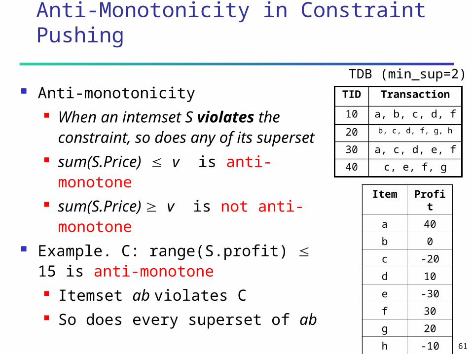
Anti-Monotonicity in Constraint Pushing
Anti-monotonicity When an intemset S violates the
constraint, so does any of its superset
sum(S.Price) v is anti-monotone sum(S.Price) v is not anti-
monotone Example. C: range(S.profit) 15 is
anti-monotone Itemset ab violates C So does every superset of ab
TransactionTID
a, b, c, d, f10
b, c, d, f, g, h20
a, c, d, e, f30
c, e, f, g40
TDB (min_sup=2)
Item Profit
a 40
b 0
c -20
d 10
e -30
f 30
g 20
h -10
62
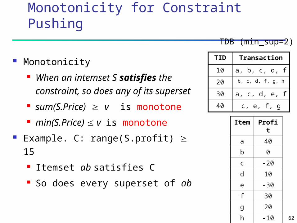
Monotonicity for Constraint Pushing
Monotonicity When an intemset S satisfies
the constraint, so does any of its superset
sum(S.Price) v is monotone min(S.Price) v is monotone
Example. C: range(S.profit) 15 Itemset ab satisfies C So does every superset of ab
TransactionTID
a, b, c, d, f10
b, c, d, f, g, h20
a, c, d, e, f30
c, e, f, g40
TDB (min_sup=2)
Item Profit
a 40
b 0
c -20
d 10
e -30
f 30
g 20
h -10

63
The Apriori Algorithm — Example
TID Items100 1 3 4200 2 3 5300 1 2 3 5400 2 5
Database D itemset sup.{1} 2{2} 3{3} 3{4} 1{5} 3
itemset sup.{1} 2{2} 3{3} 3{5} 3
Scan D
C1L1
itemset{1 2}{1 3}{1 5}{2 3}{2 5}{3 5}
itemset sup{1 2} 1{1 3} 2{1 5} 1{2 3} 2{2 5} 3{3 5} 2
itemset sup{1 3} 2{2 3} 2{2 5} 3{3 5} 2
L2
C2 C2
Scan D
C3 L3itemset{2 3 5}
Scan D itemset sup{2 3 5} 2

64
Naïve Algorithm: Apriori + Constraint
TID Items100 1 3 4200 2 3 5300 1 2 3 5400 2 5
Database D itemset sup.{1} 2{2} 3{3} 3{4} 1{5} 3
itemset sup.{1} 2{2} 3{3} 3{5} 3
Scan D
C1L1
itemset{1 2}{1 3}{1 5}{2 3}{2 5}{3 5}
itemset sup{1 2} 1{1 3} 2{1 5} 1{2 3} 2{2 5} 3{3 5} 2
itemset sup{1 3} 2{2 3} 2{2 5} 3{3 5} 2
L2
C2 C2
Scan D
C3 L3itemset{2 3 5}
Scan D itemset sup{2 3 5} 2
Constraint:
Sum{S.price < 5}

65
The Constrained Apriori Algorithm: Push an Anti-monotone Constraint Deep
TID Items100 1 3 4200 2 3 5300 1 2 3 5400 2 5
Database D itemset sup.{1} 2{2} 3{3} 3{4} 1{5} 3
itemset sup.{1} 2{2} 3{3} 3{5} 3
Scan D
C1L1
itemset{1 2}{1 3}{1 5}{2 3}{2 5}{3 5}
itemset sup{1 2} 1{1 3} 2{1 5} 1{2 3} 2{2 5} 3{3 5} 2
itemset sup{1 3} 2{2 3} 2{2 5} 3{3 5} 2
L2
C2 C2
Scan D
C3 L3itemset{2 3 5}
Scan D itemset sup{2 3 5} 2
Constraint:
Sum{S.price < 5}

66
The Constrained Apriori Algorithm: Push Another Constraint Deep
TID Items100 1 3 4200 2 3 5300 1 2 3 5400 2 5
Database D itemset sup.{1} 2{2} 3{3} 3{4} 1{5} 3
itemset sup.{1} 2{2} 3{3} 3{5} 3
Scan D
C1L1
itemset{1 2}{1 3}{1 5}{2 3}{2 5}{3 5}
itemset sup{1 2} 1{1 3} 2{1 5} 1{2 3} 2{2 5} 3{3 5} 2
itemset sup{1 3} 2{2 3} 2{2 5} 3{3 5} 2
L2
C2 C2
Scan D
C3 L3itemset{2 3 5}
Scan D itemset sup{2 3 5} 2
Constraint:
min{S.price <= 1 }

67
Chapter 5: Mining Association Rules in Large Databases
Association rule mining
Algorithms for scalable mining of (single-dimensional
Boolean) association rules in transactional databases
Mining various kinds of association/correlation rules
Constraint-based association mining
Sequential pattern mining
Applications/extensions of frequent pattern mining
Summary

68
Sequence Databases and Sequential Pattern Analysis
Transaction databases, time-series databases vs. sequence databases
Frequent patterns vs. (frequent) sequential patterns Applications of sequential pattern mining
Customer shopping sequences: First buy computer, then CD-ROM, and then digital
camera, within 3 months. Medical treatment, natural disasters (e.g., earthquakes),
science & engineering processes, stocks and markets, etc.
Telephone calling patterns, Weblog click streams DNA sequences and gene structures

69
What Is Sequential Pattern Mining?
Given a set of sequences, find the complete set of frequent subsequences
A sequence database
A sequence : < (ef) (ab) (df) c b >
An element may contain a set of items.Items within an element are unorderedand we list them alphabetically.
<a(bc)dc> is a subsequence of <<a(abc)(ac)d(cf)>
Given support threshold min_sup =2, <(ab)c> is a sequential pattern
SID sequence
10 <a(abc)(ac)d(cf)>
20 <(ad)c(bc)(ae)>
30 <(ef)(ab)(df)cb>
40 <eg(af)cbc>

70
Challenges on Sequential Pattern Mining
A huge number of possible sequential patterns are hidden in databases
A mining algorithm should find the complete set of patterns, when
possible, satisfying the minimum support (frequency) threshold
be highly efficient, scalable, involving only a small number of database scans
be able to incorporate various kinds of user-specific constraints

71
Studies on Sequential Pattern Mining
Concept introduction and an initial Apriori-like algorithm R. Agrawal & R. Srikant. “Mining sequential patterns,” ICDE’95
GSP—An Apriori-based, influential mining method (developed at IBM Almaden)
R. Srikant & R. Agrawal. “Mining sequential patterns: Generalizations and performance improvements,” EDBT’96
From sequential patterns to episodes (Apriori-like + constraints) H. Mannila, H. Toivonen & A.I. Verkamo. “Discovery of
frequent episodes in event sequences,” Data Mining and Knowledge Discovery, 1997
Mining sequential patterns with constraints M.N. Garofalakis, R. Rastogi, K. Shim: SPIRIT: Sequential
Pattern Mining with Regular Expression Constraints. VLDB 1999

72
Sequential pattern mining: Cases and Parameters
Duration of a time sequence T Sequential pattern mining can then be confined to
the data within a specified duration Ex. Subsequence corresponding to the year of 1999 Ex. Partitioned sequences, such as every year, or
every week after stock crashes, or every two weeks before and after a volcano eruption
Event folding window w If w = T, time-insensitive frequent patterns are found If w = 0 (no event sequence folding), sequential
patterns are found where each event occurs at a distinct time instant
If 0 < w < T, sequences occurring within the same period w are folded in the analysis

73
Example
When event folding window is 5 munites Purchases within 5 munits is considered to
be taken together

74
Sequential pattern mining: Cases and Parameters (2)
Time interval, int, between events in the discovered pattern
int = 0: no interval gap is allowed, i.e., only strictly consecutive sequences are found
Ex. “Find frequent patterns occurring in consecutive weeks”
min_int int max_int: find patterns that are separated by at least min_int but at most max_int
Ex. “If a person rents movie A, it is likely she will rent movie B within 30 days” (int 30)
int = c 0: find patterns carrying an exact interval Ex. “Every time when Dow Jones drops more than 5%,
what will happen exactly two days later?” (int = 2)

75
A Basic Property of Sequential Patterns: Apriori
A basic property: Apriori (Agrawal & Sirkant’94) If a sequence S is not frequent Then none of the super-sequences of S is frequent E.g, <hb> is infrequent so do <hab> and <(ah)b>
<a(bd)bcb(ade)>50
<(be)(ce)d>40
<(ah)(bf)abf>30
<(bf)(ce)b(fg)>20
<(bd)cb(ac)>10
SequenceSeq. ID Given support threshold min_sup =2
76
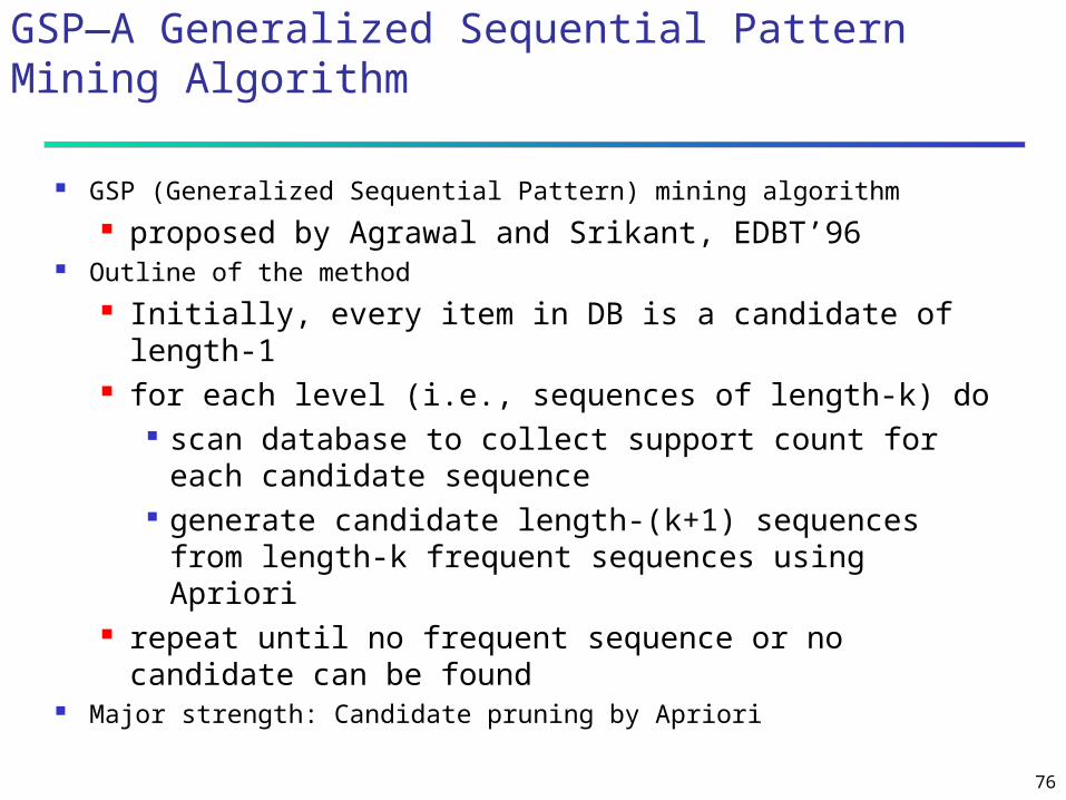
GSP—A Generalized Sequential Pattern Mining Algorithm
GSP (Generalized Sequential Pattern) mining algorithm proposed by Agrawal and Srikant, EDBT’96
Outline of the method Initially, every item in DB is a candidate of length-
1 for each level (i.e., sequences of length-k) do
scan database to collect support count for each candidate sequence
generate candidate length-(k+1) sequences from length-k frequent sequences using Apriori
repeat until no frequent sequence or no candidate can be found
Major strength: Candidate pruning by Apriori

77
Finding Length-1 Sequential Patterns
Examine GSP using an example Initial candidates: all singleton sequences
<a>, <b>, <c>, <d>, <e>, <f>, <g>, <h>
Scan database once, count support for candidates
<a(bd)bcb(ade)>50
<(be)(ce)d>40
<(ah)(bf)abf>30
<(bf)(ce)b(fg)>20
<(bd)cb(ac)>10
SequenceSeq. ID
min_sup =2
Cand Sup
<a> 3
<b> 5
<c> 4
<d> 3
<e> 3
<f> 2
<g> 1
<h> 1

78
Generating Length-2 Candidates
<a> <b> <c> <d> <e> <f>
<a> <aa> <ab> <ac> <ad> <ae> <af>
<b> <ba> <bb> <bc> <bd> <be> <bf>
<c> <ca> <cb> <cc> <cd> <ce> <cf>
<d> <da> <db> <dc> <dd> <de> <df>
<e> <ea> <eb> <ec> <ed> <ee> <ef>
<f> <fa> <fb> <fc> <fd> <fe> <ff>
<a> <b> <c> <d> <e> <f>
<a> <(ab)> <(ac)> <(ad)> <(ae)> <(af)>
<b> <(bc)> <(bd)> <(be)> <(bf)>
<c> <(cd)> <(ce)> <(cf)>
<d> <(de)> <(df)>
<e> <(ef)>
<f>
51 length-2Candidates
Without Apriori property,8*8+8*7/2=92 candidates
Apriori prunes 44.57% candidates

80
Generating Length-3 Candidates and Finding Length-3 Patterns
Generate Length-3 Candidates Self-join length-2 sequential patterns
Based on the Apriori property <ab>, <aa> and <ba> are all length-2 sequential
patterns <aba> is a length-3 candidate <(bd)>, <bb> and <db> are all length-2
sequential patterns <(bd)b> is a length-3 candidate
46 candidates are generated Find Length-3 Sequential Patterns
Scan database once more, collect support counts for candidates
19 out of 46 candidates pass support threshold

81
The GSP Mining Process
<a> <b> <c> <d> <e> <f> <g> <h>
<aa> <ab> … <af> <ba> <bb> … <ff> <(ab)> … <(ef)>
<abb> <aab> <aba> <baa> <bab> …
<abba> <(bd)bc> …
<(bd)cba>
1st scan: 8 cand. 6 length-1 seq. pat.
2nd scan: 51 cand. 19 length-2 seq. pat. 10 cand. not in DB at all
3rd scan: 46 cand. 19 length-3 seq. pat. 20 cand. not in DB at all
4th scan: 8 cand. 6 length-4 seq. pat.
5th scan: 1 cand. 1 length-5 seq. pat.
Cand. cannot pass sup. threshold
Cand. not in DB at all
<a(bd)bcb(ade)>50
<(be)(ce)d>40
<(ah)(bf)abf>30
<(bf)(ce)b(fg)>20
<(bd)cb(ac)>10
SequenceSeq. ID
min_sup =2

82
Definition c is a contiguous subsequence of a sequence s:{s1,s2,...,sn} if c is derived by dropping an item from s1 or
sn
c is derived by dropping an item from si which has at least 2 items
c’ is a contiguous subsequence of c and c is a contiguous subsequence of s
Ex: s:{ (1,2),(3,4),5,6} { 2,(3,4),5}, { (1,2),3,5,6},{ (3,5} are but { (1,2),(3,4),6},{ (1,5,6} are not

83
Candidate genration
Step 1: Join Step Lk-1 join with Lk-1 to give Ck
s1 and s2 are joined if dropping first item of s1 and last item of s2 gives the same sequence
s1 is extended by adding the last item of s2
Step 2: Prune Step Delete candidate sequences having (k-1) contiguous subsequences whose support count is less than min_support count

84
L3 C4 L4 {(1,2),3} {(1,2),(3,4)} {(1,2),(3,4)} {(1,2),4} {(1,2),3,5} {1,(3,4)} {(1,3),5} {2,(3,4)} {2,3,5}
{(1,2),3} joined with {2,(3,4)} to give {(1,2),(3,4)} {(1,2),3} joined with {2,3,5} to give {(1,2),3,5} {(1,2),3,5} is dropped since its 3 contiguous
subseq {(1,3,5} not in L3

86
Bottlenecks of GSP
A huge set of candidates could be generated
1,000 frequent length-1 sequences generate length-2
candidates!
Multiple scans of database in mining
Real challenge: mining long sequential patterns
An exponential number of short candidates A length-100 sequential pattern needs 1030
candidate sequences!
500,499,12
999100010001000
30100100
1
1012100
i i


