Page 1
1
Developing Real Option Game Models
Alcino Azevedo1,2
* and Dean Paxson**
*Hull University Business School
Cottingham Road, Hull HU6 7RX, UK
**Manchester Business School
Booth Street West, Manchester M15 6PB, UK
June, 2011
1 Corresponding author: [email protected] ; +44(0)1482463107.
2 Acknowledgments: We thank Roger Adkins, Peter Hammond, Wilson Koh, Helena Pinto, Lenos Trigeorgis,
Martin Walker, and participants at the Real Options Conference Rome 2010 and the Seminar at the Centre for
International Accounting and Finance Research, HUBS 2010, for comments on earlier versions. Alcino
Azevedo gratefully acknowledges Fundação Para a Ciência e a Tecnologia.
Page 2
2
Developing Real Option Game Models
Abstract
By mixing concepts from both game theoretic analysis and real options theory, an investment
decision in a competitive market can be seen as a “game” between firms, as firms implicitly take
into account other firms’ reactions to their own investment actions. We review several real option
game models, suggesting which critical problems have been “solved” by considering game theory,
and which significant problems have not been adequately addressed. We provide some insights on
the plausible empirical applications, or shortfalls in applications to date, and suggest some
promising avenues for future research.
keywords: Real Option Games, Games of Investment Timing, Pre-emption, War of Attrition.
Page 3
3
1. Introduction
An investment decision in competitive markets is a “game” among firms, since in making
investment decisions, firms implicitly take into account what they think will be the other firms’
reactions to their own investment actions, and they know that their competitors think the same way.
Consequently, as game theory aims to provide an abstract framework for modeling situations
involving interdependent choices, and real options theory is appropriate for most investment
decisions, a merger between these two theories appears to be a logic step.
The first paper in the real options literature to consider interactions between firms was Frank Smets
(1993), who created a new branch of real option models taking into account the interactions
between firms.
In the current literature, a “standard” real option game (“SROG”) model is where the value of the
investment is treated as a state variable that follows a known process3; time is considered infinite
and continuous; the investment cost is sunk, indivisible and fixed4; firms are not financially
constrained; the investment problem is studied in isolation as if it were the only asset on the firm’s
balance sheet5 (i.e., the game is played on a single project); and there are usually two firms holding
the option to invest6 (duopoly). The focus of the analysis is the derivation of the firms’ value
functions and their respective investment thresholds, under the assumption that either firms are risk-
neutral or the stochastic evolution of the variable(s) underlying the investment value is spanned by
the current instantaneous returns from a portfolio of securities that can be traded continuously
without transaction costs in a perfectly competitive capital market.
The two most common investment games are the “pre-emption game” and the “war of attrition
game”, both usually formulated as “zero-sum games”. In the pre-emption game, it is assumed that
there is a first-mover advantage that gives firms an incentive to be the first to invest. In the attrition
game, it is assumed that there is a second-mover advantage that gives firms an incentive to be the
3 Typically, geometric Brownian motion (gBm) and mean reverting processes, stochastic processes with
jumps, birth and death processes, or combinations of these processes. 4 There are papers, however, where this assumption is relaxed. See, for instance, Robert Pindyck (1993),
where it is assumed that due to physical difficulties in completing a project, which can only be resolved as the
project proceeds, and to uncertainty about the price of the project inputs, the investment costs are uncertain;
see also Avinash Dixit and Pindyck (1994), chapter 6, where, in a slightly different context, the same
assumption is made. 5 This is a weakness of the SROG models in the sense that the full dynamics of an industry is not analyzed.
Joseph Williams (1993) and Fridick Baldursson (1998), who analyze the dynamics of oligopolistic industries,
are exceptions to this rule. 6 See Romain Bouis, Kuno Huisman and Peter Kort (2009) for an example of a real options model with three
firms.
Page 4
4
second to invest. Furthermore, typically the firm’s advantage to invest first/second is assumed to be
partial7 (i.e., the investment of the leader (pre-emption) or the follower (war of attrition) does not
completely eliminate the revenues of its opponent); the investment game is treated as a “one-shot
game (i.e., firms are allowed to invest only once) where firms are allowed to invest (play) either
sequentially or simultaneously, or both; cooperation between firms is not allowed; the market for
the project, underlying the investment decision, is considered to be complete and frictionless; and
firms are assumed to be ex-ante symmetric and ex-post either symmetric or asymmetric, and can
only improve their profits by reducing the profits of rivals (zero-sum game).
In addition, in a SROG model8, the way the firm’s investment thresholds are defined, in the firm’s
strategy space, depends on the number of underlying variables used. Thus, in models that use just
one underlying variable, the firm’s investment threshold is defined by a point; in models that use
two underlying variables, the firm’s investment threshold is defined by a line; and in models that
use three or more underlying variables, the firm’s investment threshold is defined by a surface or
other more complex space structures. However, regardless of the number of underlying variables
used in the real options model, the principle underlying the use of the investment threshold(s),
derived through the real options valuation technique, remains the same: “a firm should invest as
soon as its investment threshold is crossed the first time”.
Non-standard ROG (“NSROG”) relax some of these assumptions and constraints. In Table 1, in the
Appendix, we summarize the types and assumptions of several NSROG.
The three most basic elements that characterize a game are the players, their strategies and payoffs.
Translating these to a ROG, the players are the firms that hold the option to invest (investment
opportunity), the strategies are the choices “invest”/”defer” and the payoffs are the firms’ value
functions. Additionally, to be fully characterized, a game still needs to be specified in terms of what
sort of knowledge (complete/incomplete) and information (perfect/imperfect,
symmetric/asymmetric) the players have at each point in time (node of the game-tree) and regarding
the history of the game; what type of game is being played (a “one-shot” game, a “zero-sum” game,
7 Exceptions to this rule are Bart Lambrecht and William Perraudin (2003) and Pauli Murto and Jussi Keppo
(2002) models, which are derived for a context of complete pre-emption. 8 By (“ROG”) we mean an investment game or activity where firms’ payoffs are derived combining game
theory concepts with the real options methodology.
Page 5
5
a sequential/simultaneous9 game, or a cooperative/non-cooperative game); and whether mixed
strategies are allowed10
.
Even though, at a first glance, the adaptability of game theory concepts to real option models seems
obvious and straightforward, there are some differences between a “standard” ROG and a
“standard” game like those which are illustrated in basic game theory textbooks.
One difference between a “standard” game and a SROG is the way the players’ payoffs are given.
In “standard” games such as the “prisoners’ dilemma”, the “grab-the-dollar”, the “burning the
bridge” or the “battle-of-the-sexes” games, the players’ payoffs are deterministic, while in SROGs
they are given by sometimes complex mathematical functions that depend on one, or more,
stochastic underlying variables. This fact changes radically the rules under which the game
equilibrium is determined, because if the players’ payoffs depend on time, and time is continuous,
the game is played in continuous-time. But, if the game is played in a continuous-time and players
can move at any time, what does the strategy “move immediately after” mean? In the real options
literature, the approach used to overcome this problem is based on Drew Fudenberg and Jean Tirole
(1985), which develops a new formalism for modeling games of timing, permitting a continuous-
time representation of the limit of discrete-time mixed-strategy equilibria11
.
In a further section, we discuss in more detail some of the most important differences, from the
point of view of the mathematical formulation of the model, between continuous-time ROG and
discrete-time ROG, as well as some potential time-consistency and formal and structure-coherence
problems which may arise in a continuous-time framework.
The main principle underlying game theory is that those involved in strategic decisions are affected
not only by their own choices but also by the decisions of others. Game theory started with the work
of John von Neumann in the 1920s, which culminated in his book with Oskar Morgenstern
published in 1944. Von Neumann and Morgenstern studied “zero-sum” games where the interests
of two players are strictly opposed. John Nash (1950, 1953) treated the more general and realistic
case of a mixture of common interests and rivalry for any number of players. Others, notably
Reinhard Selten and John Harsanyi (1988), studied even more complex games with sequences of
moves and games with asymmetric information.
9 In real option sequential games, the players’ payoffs depend on time and are usually called the “Leader” and
the “Follower” value functions. 10
The papers reviewed here are organized according to all of these categories in table 2, by author
contributions. 11
Fudenberg and Tirole (1985) contributions to real option game models are discussed in section 2.
Page 6
6
With the development of game theory, a formal analysis of competitive interactions became
possible in economics and business strategy. Game theory provides a way to think about social
interactions of individuals, by bringing them together and examining the equilibrium of the game in
which these strategies interact, on the assumption that every person (economic agent) has his own
aims and strategies. There are four main specifications for a game: the players, the actions available
to them, the timing of these actions and the payoff structure of each possible outcome. The players
are assumed to be rational (i.e., each player is aware of the rationality of the other players and acts
accordingly) and their rationality is accepted as a common knowledge12
. Once the structure of a
game understood and the strategies of the players set, the solution of the game can be determined
using Nash (1950, 1953), which uses novel mathematical techniques to prove the existence of
equilibrium in a very general class of games.
Game-theoretic models can be divided into games with or without “perfect information” and with or
without “complete information”. “Perfect information” means that the players know all previous
decisions of all the players in each decision node; “complete information” means that the complete
structure of the game, including all the actions of the players and the possible outcomes, is common
knowledge13
. Sometimes, it may be unclear to each firm where its rival is at each point in time and
so the assumption of complete information may not be realistic14
. In addition, games can also be
classified according to whether cooperation among players is allowed or not. In the former case, the
game is called a “cooperative game”, in the later, it is called a “non-cooperative game”. In “non-
cooperative games” it is assumed that players cannot make a binding agreement. That is, each
cooperative outcome must be sustained by Nash equilibrium strategies. On the other hand, in
“cooperative games”, firms have no choice but to cooperate. Many real life investment situations
exhibit both cooperative and non-cooperative features.
The Nash equilibrium is a concept commonly used in the real options literature. Translated to real
option game models, when competing for the revenues from an investment, if firms reach a point
where there is a set of strategies with the property that no firm can benefit by changing its strategy
12
Note that, although game theory assumes rationality on the part of the players in a game, people may act in
imperfectly rational ways. There are many unexplained phenomena assuming rationality. However, in
business and economic decisions, this assumption may be a good start for gaining a better understanding of
what is going on around us. 13
The distinction between incomplete and imperfect information is somewhat semantic (see Tirole (1988), p.
174, for more details). For instance, in R&D investment games, firms may have “incomplete information”
about the quality or success of each other’s research effort and “imperfect information” about how much their
rivals have invested in R&D. 14
It is quite common, for instance, that a firm, before an investment decision, is uncertain about the strategic
implications of its action, such as whether it will make its rival back down or reciprocate, whether its rival
will take it as a serious threat or not.
Page 7
7
while its opponent keeps its strategies unchanged, then that set of strategies, and the corresponding
firms’ payoffs, constitute a Nash equilibrium. This notion captures a steady state of the play of a
strategic game in which each firm holds the correct expectation about its rival’s behavior and acts
rationally. Although seldom used in the real options literature, the notion of a real option “mixed
strategy Nash equilibrium” is designated to model a steady state investment game in which firms’
choices are not deterministic but regulated by probabilistic rules. In this case we study a real option
Bayesian Nash equilibrium, which, in its essence, is the Nash equilibrium of the Bayesian version
of the real option game, i.e., the Nash equilibrium we obtain when we consider not only the
strategic structure of the real option game but also the probability distributions over the firms’
different (potential) characters or types. For instance, consider a N-firm real option game. A
Bayesian version of this game consists of: i) a finite set of potential types for each firm, ii) a finite
set of perfect information games, each corresponding to one of the potential combinations of the
firms’ different types and, iii) a probability distribution over a firm’s type, reflecting the beliefs of
its opponents about its true type.
A game can be represented in a “normal-form” or in an “extensive-form”. In the “normal-form
representation”, each player, simultaneously, chooses a strategy, and the combination of the
strategies chosen by the players determines a payoff for each player. In the “extensive-form
representation” we specify: (i) the players in the game, (ii) when each player has the move, (iii)
what each player can do at each opportunity to move, (iv) what each player knows at each
opportunity to move, and (v) the payoff received by each player for each combination of moves that
can be chosen by players15
.
In our review we select an extensive number of papers, published or in progress, modeling
investment decisions considering uncertainty and competition, developed over the last two decades.
Our goal is to highlight many of the contributions to the literature on ROG, relate these results to
the known empirical evidence, if any, and suggest new avenues for future research.
This paper is organized as follows. In section 2, we introduce basic aspects of the SROG models,
discuss the mathematical formulation, principles and methodologies commonly used, such as the
derivation of the firms’ payoffs, and respective investment thresholds, and the determination of
firms’ dominant strategies and game equilibrium(a). In addition, we analyze, and contrast, the
differences between discrete-time real option games and continuous-time real option games. In
section 3, as a complement to our discussions, we briefly introduce real option-related literature,
15
For a detailed description about game representation techniques see Robert Gibbons (1992), pp. 2-12, for
the normal-form representation, and pp. 115-129, for the extensive-form representation.
Page 8
8
namely, “continuous-time games of timing” and “deterministic” and “stochastic” investment
models. Section 4 reviews two decades of academic research on “standard” and “non standard”
ROG models. Tables 1 and 2, in the Appendix, classify these articles by game characteristics.
Section 5 surveys the limited empirical research and suggests some testable hypotheses. Section 6
concludes and suggests new avenues for research.
2. Real Option Game Framework
We first review standard monopoly real option models, and then provide the basic framework for
standard strategic real option models.
2.1 Monopoly Market
The standard real option model for a monopoly market can be described as follows: there is a single
firm with the possibility of investing I in a project that yields a flow of income tX , where tX
follows a gBm process given by equation (1).
t X t X tdX X dt X dz (1)
where, X is the instantaneous conditional expected percentage change in tX per unit of time
(also known as the drift) and X is the instantaneous conditional standard deviation per unit of
time in tX (also known as the volatility). Both of these variables are assumed to be constant over
time and the condition X r holds, where r is the riskless interest rate, and dz is the increment of
a standard Wiener process for the variable tX . Given the assumptions above, using standard real
options procedures the derivation of the firm’s value function and investment threshold is
straightforward (see Robert McDonald and Daniel Siegel, 1986).
The firm’s value function is given by (for simplicity of notation we neglect the subscript t in the
variable X):
*
*
if ( )
if
AX X XF X
X I X X
(2)
with,
1 1
1 1 1A
I
(3)
Page 9
9
I is the constant investment cost, and is the positive root of the following quadratic function:
211 0
2r r (4)
that is,
2
2 2 2
1 ( ) ( ) 1 2 1
2 2
r r r
(5)
with Xr .
The firm’s optimal investment strategy consists in investing as soon as tX first crosses *X , where
*X is given by equation (6):
*
1X I
(6)
Since 1 , the investment rule specifies that the firm should not invest before the value of the
project has exceeded I by a certain mark-up margin.
This is the fundamental result from irreversible investment analysis under uncertainty. The essence
of the investment timing strategy is to find a critical project value, *X , at which the value from
postponing the investment further equals the net present value of the project X I . As soon as this
value (investment threshold) is reached, the firm should invest. Since this is the solution for a
monopoly market, the investment threshold, *X , is sometimes referred to in the literature as the
“non-strategic investment threshold”, recognizing the fact that it is the firm’s optimal threshold
value on the assumption that its payoff is independent of other firms’ actions16
.
2.2 Duopoly Market
In the real options literature there are models concerned with an exclusive (monopolistic) projects,
in the sense that only one firm holds the opportunity to invest, and models concerned with non-
exclusive projects, leading usually to sequential investments (leader/follower models). The former
case, characterizes a game of one firm against nature, the later characterizes a standard ROG.
16
Note, however, that investments in large projects in monopoly markets can have an effect on the value of
the monopolistic firm similar to the entrance of a new competitor. For instance, Jussi Keppo and Hao Lu
(2003) derived a real options model for a monopolistic electricity market where due to the size of the new
electricity plant, its operation will affect the market supply and the path of the electricity prices, and
consequently, the value of the firm’s currently active projects.
Page 10
10
Ideally, in ROG models the choice regarding leadership in the investment should be endogenous to
the derivation of the firms’ value functions and investment thresholds and the determination of the
equilibrium(a) of the game. However, the mathematics for doing so are complex and, consequently,
in the real options literature, so far, the approach that has been followed in this regard has been to
assign, deterministically or by flipping a coin, the leader and the follower roles17
.
Consider an industry comprised of two identical firms, where each firm possesses an option to
invest in the same (and unique) project that will produce a unit of output18
. Furthermore, assume
that the cost of the investment is I and irreversible and the cash flow stream from the investment is
uncertain. In such context the payoff of each firm is affected by the actions (strategy) of its
opponent. Then consider the extreme case where not only the project is unique but also as soon as
one firm invests, it becomes worthless for the firm which has not invested, i.e., at time t when one
firm triggers its investment, the investment opportunity is completely lost for the other firm.
Consequently, due to the fear of losing the investment opportunity, each firm has a strong incentive
to invest before its opponent as long as its payoff is positive. Hence, firms have an incentive to
invest earlier than suggested by the monopoly solution (6).
Avinash Dixit and Robert Pindyck (1994), chapter 9, Kuno Huisman (2001), Dean Paxson and
Helena Pinto (2005), among others, developed real option models for leader/follower competition
settings. In these models, at a first moment of the investment game, only one firm invests and
becomes the leader, achieving a (perhaps temporary) monopolist payoff; in a subsequent moment, a
second firm is allowed to invest if that becomes optimal, and becomes the follower, with both firms
thereafter sharing the payoff of a duopoly market. More specifically, assume that the firms’ revenue
flow is given by (7),
,( )i jk kX t D
(7)
where ( )X t is the market revenue flow and ,i jk kD is a deterministic factor representing the
proportion of the market revenue allocated to each firm for each investment scenario, with
, ,i j L F , where L means “leader” and F “follower”, and 0,1k , where 0 means that firm is
not active and 1 means that firm is active.
17
Williams (1993) and Steven Grenadier (1996) are among the few exceptions to this rule. 18
In this section we rely on Smets (1993).
Page 11
11
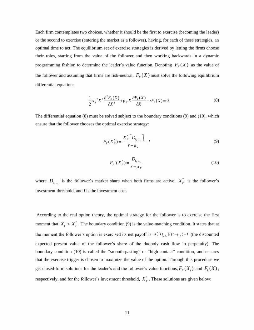
Each firm contemplates two choices, whether it should be the first to exercise (becoming the leader)
or the second to exercise (entering the market as a follower), having, for each of these strategies, an
optimal time to act. The equilibrium set of exercise strategies is derived by letting the firms choose
their roles, starting from the value of the follower and then working backwards in a dynamic
programming fashion to determine the leader’s value function. Denoting ( )FF X as the value of
the follower and assuming that firms are risk-neutral, ( )FF X must solve the following equilibrium
differential equation:
22 2
2
( ) ( )1( ) 0
2
F FX X F
F X F XX X rF X
X X
(8)
The differential equation (8) must be solved subject to the boundary conditions (9) and (10), which
ensure that the follower chooses the optimal exercise strategy:
*
1 ,1*( ) F LF
F F
x
X DF X I
r
(9)
1 ,1*'( ) F L
F F
X
DF X
r
(10)
where 1 ,1F L
D is the follower’s market share when both firms are active, *
FX is the follower’s
investment threshold, and I is the investment cost.
According to the real option theory, the optimal strategy for the follower is to exercise the first
moment that *
t FX X . The boundary condition (9) is the value-matching condition. It states that at
the moment the follower’s option is exercised its net payoff is *
1 ,1[ ] / ( )F LF XX D r I (the discounted
expected present value of the follower’s share of the duopoly cash flow in perpetuity). The
boundary condition (10) is called the “smooth-pasting” or “high-contact” condition, and ensures
that the exercise trigger is chosen to maximize the value of the option. Through this procedure we
get closed-form solutions for the leader’s and the follower’s value functions, ( )F tF X and ( )LF X ,
respectively, and for the follower’s investment threshold, *
FX . These solutions are given below:
Page 12
12
*
*
1 ,1 *
if 1
( )[ ]
if F L
F
F
F
F
X
I XX X
XF X
X DI X X
r
(11)
*
1 ,11F L
XF
rX I
D
(1 2)
And,
1 ,0 1 ,1 1 ,0 *
*
1 ,1
1 ,1 *
[ ] [ ] if
1( )
[ ] if
L F L F L F
L F
L F
F
X F
L
F
X
X D D D XI X X
r D XF X
X DX X
r
(13)
where 1 ,0L F
D and 1 ,1L F
D are the leader’s market shares when it is alone in the market and when it is
active with the follower, respectively.
The expression for the leader’s investment threshold, *
LX , is derived by equalizing, for *
FX X ,
expressions (11) and (13), replacing variable X by *
LX and solving the resulting equation for *
LX .
Finally, when both firms invest simultaneously they will share the duopoly cash flow in perpetuity
given by equation (14).
( ) ( )1 ,1
( )
[ ]( )
L F F L
L F
X
X DF X I
r
(14)
In the real options literature there are models for duopoly markets, such as Pauli Murto and Jussi
Keppo (2002), where simultaneous investment is not allowed. In such cases, without any loss of
insight, we can assume that “if the two firms want to invest simultaneously, then the one with the
highest value, X , gets the project; if the project has the same value for both firms and both want to
invest at the same time, the one who gets the project is chosen randomly using an even uniform
distribution.” With few exceptions, in the literature it is generally assumed that both players can
Page 13
13
observe all the parameters of the model (drift, volatility, etc) and the evolution of the random
variable dz given in (1) 19
.
2.2.1 Competition Setting
The Smets (1993) framework consists in the (deterministic) definition of a certain number of
competition factors, each assigned to a particular investment scenario, all governed by an
inequality. These competition factors, and the respective inequality, are the key elements in the
determination of the firms’ dominant strategy at each node of the game-tree and the resultant
equilibrium of the game.
2.2.2 Dominant Strategies and Game Equilibrium
For a standard duopoly pre-emption game, the formulation of the game setting can be described as
follows: there are two idle firms, each with two strategies available “invest”/”defer” which can lead
to three different game scenarios: (i) both firms inactive; (ii) one firm, the leader, active and the
other firm, the follower, inactive; (iii) both firms active, with the leader the first to invest. To each
of these investment scenarios correspond different firms’ payoffs, given by equation (17),
conditioned by one (or several) competition factors governed by an inequality similar to the one
below:
1 0 11 0 0i j i j i jD D D (15)
The competition factors are represented by i jk kD , with k 0,1 , where “zero” means inactive,
“one” means active20
and i, in this case, denotes the leader (L) and j denotes the follower (F).
Following the notation above, we can redefine inequality (15) for each of the firms. For the leader it
would be:
1 0 1 1 0 0L F L F L FD D D
(16)
19
Two exceptions are Jean-Paul Décamps, Mariotti, and Stéphane Villeneuve (2002), who studied a
competitive investment problem where firms have imperfect information regarding those variables, and
Ariane Reiss (1998) who derived a real option model for a patent race where the actions of the investors are
formulated in a non-game theoretic framework. 20
Note that this notation allows models with a wider range of investment scenarios. For instance, in Alcino
Azevedo and Paxson (2009), i jk kD is defined with k 0,1,2,12 , with “0” and “1” meaning the same as
above, and “2” and “12” representing investment scenarios where firms are active but with, respectively,
technology 2 alone and both technology 1 and technology 2 at the same time.
Page 14
14
The economic interpretation for the relationship between the first two factors, 1 0 1 1L F L F
D D , is that
the leader’s revenue market share is higher when operating alone than when operating with the
follower; the economic interpretation for the relationship between the second and the third
factors,1 1 0 0L F L F
D D , is that the leader’s market share is higher when it operates with the follower
than when it is idle. Note that in a duopoly, the market share of the follower is a complement of the
leader’s. Hence, 1F L L Fk k k kD D . Therefore, for the follower, inequality (17) holds.
1 1 0 0 0 1F L F L F LD D D
(17)
After the definition of the competition factors, their economic meaning and the inequality that
govern the relationship between the competition factors, we can determine at each node of the
investment game-tree, the firms’ dominant strategy, and study the equilibrium of the game. Note
that the example used above is a “zero-sum pre-emption game” with the two firms competing for a
percentage of the market revenues, where for each investment scenario, the dominate share is
deterministically assigned to the leader, and the follower is given a proportion of the total market
revenues upon entry (see Andrianos Tsekrekos, 2003). These deterministic competition factors can
take more sophisticated forms and different meanings, but, essentially, the framework described
above to derive the firms’ payoffs, determine the dominant strategies at each node of the investment
game-tree, and study the equilibrium of the game is the same.
Figure 1 illustrates the relationship between the leader’s competition factors and the firms’
investment thresholds.
0 0L F
D 1 0L F
D 1 1L F
D
Time 0 *
1LX
*
1FX
Figure 1 – Duopoly Pre-emption Game: Leader/Follower Investment Thresholds
2.2.3 The Firms’ Payoffs
Using the general form for the representation of the firms’ values as a function of t, with 0t at
the beginning of the game, the firms’ revenue flow is given by:
Page 15
15
k k i ji j t k kF X D
(18)
where, tX is the underlying variable (for instance, market revenues); i jk kD represents the
competition factors, with k 0,1 , where “0” means that the firm to which is assigned this
competition factor is inactive and “1” means that the firm is active, with i, j denoting the leader (L)
or the follower (F).
The existence of a first mover’s advantage (pre-emption game) is one assumption underlying the
derivation of the SROG model, and so there is no need to make this assumption explicit in the
inequality. However, in order to do so we just need to introduce a new pair of competition factors in
inequality (16), 1 1 1 1L F F LD D , and it would become 1 0 1 1 1 1 0 0L F L F F L L F
D D D D with the second and
third competition factors ensuring that the market revenue share of the leader, 1 1L FD , is greater than
that of the follower, 1 1F LD , when both firms are active.
This framework also allows for the treatment of other types of investment games, such as a second
mover’s advantage context (war of attrition game). In addition, the first mover’s advantage can be
set as temporary or permanent. If permanent, we assume that inequality (16) holds forever, i.e., as
soon as the follower enters the market, both firms share the market revenues in a static and pre-
defined way, governed by the competition factors and the respective investment game inequality,
with an advantage for the leader. If temporary, it is assumed that, at some stage of the game, with
both firms active, a new market share arrangement will take place, reducing, or even eliminating,
the leader’s initial market share advantage. New entries or exits of existing players are not allowed.
The firms’ value functions (payoffs) can incorporate one or several competition factors and, as
mentioned earlier, a key parameter for the comparison of the firms’ payoffs, at each node of the
game-tree, is (are) the competition factor(s), which determines the payoff assigned to each firm and
investment strategies available. The information underlying each competition factor/game
inequality is then transposed to the firms’ payoffs and allows the determination of the firms’
dominant strategy at each node of the game-tree. When the leader is active and the follower is idle,
the leader’s payoff function is:
1 0 1 0L FL F tF X D (19)
Following similar procedures as those described above, the payoff functions for the leader and the
follower when both firms are active are given, respectively, by:
Page 16
16
1 1 1 1L FL F tF X D (20)
1 1 1 1F LF L tF X D (21)
Going back to inequality (16) we can see that 1 0 1 1L F L FD D and 1 1 1 1L F F L
D D , hence 1 0 1 1
L F L FF F
and 1 1 1 1
L F F LF F . Similar rationale is used to determine firms’ dominant strategies at each node of
the game-tree and the equilibrium of the game. Both firms are assumed to have common knowledge
about inequality (16).
2.2.4 Two-Player Pre-emption Game
The pre-emption game is one of the most common games used in the real option literature, usually
formulated as a two-player game where investment costs are sunk, firms’ payoffs uncertain, time is
assumed to be continuous and the horizon of the investment game infinite. Real options theory
shows that when an investor has a monopoly over an investment opportunity, where the investment
cost is sunk and the revenues are uncertain, there is an option value to wait which is an incentive to
delay the investment opportunity more than the net present value methodology suggests. The more
uncertain are the revenues, the more valuable is the option to wait. However, when competition is
introduced into the investment problem, for a ceteris paribus analysis, the intuition is that the value
of the option to wait erodes. The higher the competition among firms, the less valuable is the option
to wait (defer) the investment.
In modeling duopoly pre-emption investment games using the combined real options and games
framework, one key element which is common to almost all ROG models is the use of the
Fudenberg and Tirole (1985) principle of rent equalization. According to this principle, the erosion
in the value of the option to defer the investment is caused by the fact that each firm fears being pre-
empted in the market by its rival due to the existence of a first mover-advantage. Consequently,
each firm knows that by investing a little earlier than its opponent, they will get a revenue
advantage. When this advantage is sufficiently high, firms will try to pre-empt each other, leading
them to invest earlier than would be the case otherwise.
Fudenberg and Tirole (1985) use the example of a new technology adoption game to illustrate the
effect of pre-emption in games of timing, showing that the threat of pre-emption equalizes rents in a
duopoly, thus the term “principle of rent equalization”. Figure 2 illustrates how this principle works.
Page 17
17
Figure 2 – Two-Player Pre-emption Game
In Figure 2, there are three different regions on the timeline: 0, A , ,A C and ,C . In the
interval 0, A the payoff of the follower is higher than that of the leader; in the interval ,A C the
payoff of the leader is higher than that of the follower; and in the interval ,C both players have
the same payoff. In addition, we can see that point B is the point at which the leader’s advantage
reaches a maximum. In absence of the pre-emption effect, the optimal investment time for the
leader would be point where the difference between its payoff and the follower’s payoff is highest
(point B). However, in a context where there is a first-mover advantage, because firms are afraid of
being pre-empted, the leader invests at point A, a point where the payoffs (rents) from being the
leader and the follower are equalized.
Note that, in the interval ,A B there are an infinite number of timing strategies that would lead to a
better payoff for the leader than the strategy to invest at time A. However, in a game where firms
have perfect, complete and symmetric information about the game, both firms know that, in the
interval ,A B , if they invest an instant before the opponent they will get a payoff advantage, and
this competition to pre-empt the rival leads both firms to target their investment at point A where
each firm has 50 percent chance of being the leader. In these cases, the leader is chosen by flipping
a coin. As soon as one firm achieves the leadership in the investment, for the follower, the optimal
time to invest is point C. After the follower investment both firms will share the market revenues in
a pre-assigned way, i.e., according to the information underlying inequality (16).
2.2.5 Discrete-time game Versus Continuous-time game
SROG are focused on symmetric, Markov, sub-game perfect equilibrium exercise strategies in
which each firm’s exercise strategy, conditional upon the other’s exercise strategy, is value-
maximizing. It is a Markov equilibrium in the sense that it is considered that the state of the
C B A
Follower’s Optimal Investment time Leader’s Optimal
Investment time
Point where the Leader’s Advantage
is highest
0
Page 18
18
decision process tomorrow is only affected by the state of the decision process today, and not by the
other states before that; and it is a “subgame perfect equilibrium” because the players’ strategies
must constitute a Nash equilibrium in every subgame of the original game.
In continuous-time games with an infinite horizon, the time index t, is defined in the domain
0,t . Hence, given the relative values of the leader and the follower for a given current value
of tX , we are allowed to construct the equilibrium set of exercise strategies for each firm. SROG are
usually formulated in continuous-time, so there is an obvious link between the literature on real
option game models and the literature on continuous-time games of timing. Below we briefly
introduce, discuss and illustrate the concept of continuous-time games and its relation with the
SROG models, relying mainly on the works of Carolyn Pitchik (1981), David Kreps and Robert
Wilson (1982a,b), Fudenberg and Tirole (1985), Partha Dasgupta and Eric Maskin (1986a,b), Leon
Simon and Maxwell Stinchcombe (1989), Stinchcombe (1992), James Bergin (1992), Prajit Dutta
and Aldo Rustichini (1995), and Rida Laraki, Eilon Solan, and Nicolas Vieille (2005).
As discussed earlier, for a sequential real options game in continuous-time, there is no definition for
“the last period” and the “next period”21
. This restricts the set of possible strategic game
equilibria22
and introduces potential time-consistency problems into real option game models. The
formulation of firms’ investment strategies in continuous-time is complex. Fudenberg and Tirole
(1985) highlight the fact that there is a loss of information inherent in representing continuous-time
equilibria as the limits of discrete-time mixed strategy equilibria. To correct this they extend the
strategy space to specify not only the cumulative probability that player i has invested, but also the
“intensity” with which each player invests at times “just after” the probability has jumped to one.
An investor’s strategy is defined as a “collection of simple strategies” satisfying an “inter-temporal
consistency condition”.
More specifically, a simple strategy for investor i in a game starting at a positive level of the
state variable is a pair of real-value functions ( ), ( ) : 0, 0, 0,1 0,1i iG satisfying
certain conditions ensuring that iG is a cumulative distribution function, and that when 0i ,
1iG (i.e., if the intensity of atoms in the interval , d is positive, the investor is sure to
21
See Fudenberg and Tirole (1985), Simon and Stinchcombe (1989) and Bergin (1992) for detailed
discussions on this problem. 22
For instance, the follower’s strategy “invest immediately after the leader” cannot be accommodated.
Page 19
19
invest by ). A collection of strategies for investor i, (.), (.)i iG , is the set of simple strategies
that satisfy inter-temporal consistency conditions.
Although this formulation uses mixed strategies, the equilibrium outcomes are equivalent to those
in which investors employ pure strategies. Consequently, the analysis will proceed as if each agent
uses a pure Markovian strategy, i.e., a stopping rule specifying a critical value or “trigger point” for
the exogenous variable at which the investor invests23
. Fudenberg and Tirole (1985) employ a
deterministic framework. Their methodology has been extended to a real option stochastic
environment.
An investment game can be represented using one of the following techniques: i) a normal-form
representation or ii) an extensive-form representation. The choice between these two types of
representation depends on the type of investment game. Figures 3 and 4 illustrate a sequential
investment game using a normal-form representation and an extensive-form representation,
respectively.
Firm j
Defer Invest
Firm i
Defer Repeat game ( ), ( )F t L tF X F X
Invest ( ), ( )L t F tF X F X ( ), ( )S t S tF X F X
Figure 3 – Normal-Form Representation: Sequential Real Option Duopoly Game
Firm i
invest defer
j j
invest defer invest defer
Payoff: firm i ( )L tF X ( )L tF X ( )F tF X ( )i tF X
Payoff: firm j ( )F tF X ( )F tF X
( )L tF X ( )i tF X ,i L F
Figure 4 – Extensive-Form Representation: Sequential Real Option Duopoly Game
23
Note that this is for convenience only given that underlying the analysis is an extended space with mixed
strategies (see Robin Mason and Helen Weeds, 2001).
Page 20
20
In Figure 3 the concept of “timing strategy”, implicit in a sequential ROG, and the sequence of the
players’ moves is not as intuitive as in Figure 4, which explains the convenience of using the
extensive-form representation to describe this type of game rather than the normal-form
representation. In both of the representations above, however, the leader’s and the follower’s
payoffs are represented by the same expressions ( )L tF X and ( )F tF X , expressions (13) and (11),
respectively. ( )S tF X , in Figure 3, is the leader’s and the follower’s payoffs when both firms invest
simultaneously, expression (14).
The subscript t in ( )L tF X , ( )F tF X and ( )S tF X , denotes the fact that X is not static but varies over
time, meaning that as time changes so do the firms’ payoffs. Consequently, in practice, for each
firm, Figures 3 and 4 display different payoffs at each instant of the game. An intuitive view of the
dynamic nature of the firms’ payoffs, “timing strategy” and the Fudenberg and Tirole (1985)
methodology of using the discrete-time framework as a proxy of the continuous-time approach is
the elaborated representation of a duopoly ROG given in Figure 5.
i
Invest Defer
j Period 0
Invest Defer Invest Defer
i
Invest Defer
j Period 1
Invest Defer Invest Defer
i
Invest Defer
j Period 2
Invest Defer Invest Defer
i
Invest Defer
j Period n
Invest Defer Invest Defer
Figure 5 – Illustrative Extensive-Form: Continuous-Time Real Option Duopoly Game
Page 21
21
An additional aspect that Figure 5 makes easier to see is the fact that in a duopoly sequential game
where firms have two strategies available (invest/defer), although they can choose the strategy
“invest” only once, they are allowed to choose the strategy “defer” an infinite number of times,
since in a continuous-time framework, in between any two instants of the game where firms do not
choose the strategy “invest”, they have chosen, theoretically, an infinite number of times the
strategy “defer”24
.
ROG models usually assume that time is infinite. This assumption is a mathematical convenience to
derive the firms’ payoffs and respective investment thresholds. However, it is not appropriate for
many investment projects. From the point of view of the equilibrium of the game, there are
differences between games where the option to invest matures at some particular point in time, and
games where the option to invest can be held in perpetuity. However, this problem has passed
“unnoticed” because the focus of our analysis has been directed not to the “timing strategy”,
chronologically speaking, but to the time at which the value of the investment (i.e., the underlying
variable) reaches a threshold, regardless at which chronological point that occurs.
Using (13) and (11) we plot, in Figure 6, the leader and the follower payoff functions, respectively,
whose shapes are standard (see Dixit and Pindyck, 1994).
Figure 6 – Firms’ Investment Thresholds for a Two-player Pre-emption Game
In Figure 6, there exists a unique point * *0,L FX X with the following properties:
*
*
* *
*
( ) ( ) if
( ) ( ) if
( ) ( ) if
( ) ( ) if
L t F t t L
L t F t t L
L t F t L t F
L t F t t F
F X F X X X
F X F X X X
F X F X X X X
F X F X X X
24
Note that this does not happen in the “The Prisoner’s Dilemma” game because it is a “simultaneous-one-
shot” game, where players can choose only once either “confess” or “defect”.
XF*
Page 22
22
which demonstrates that there is a unique value at which the payoffs to both the leader and the
follower are equal. At any point below *
LX each firm prefers to be the follower; at *
LX the benefits
of a potentially temporary monopoly just equal the costs of paying the exercise price earlier; at any
point above between *
LX and *
FX each firm prefers to be the leader; for *
t FX X , the value of
leading, following or simultaneous exercise are equal (see Grenadier (1996), p. 1661 and p. 1678
for a formal proof).
Figure 6 shows the results for a scenario where after the follower investment both firms share a
(permanent) symmetric market share (the initial leader’s advantage is eliminated). Hence, both the
leader’s and the follower’s payoff functions overlap each other for * ,t FX X . However, notice
that the framework above allows, through inequality (16), any other market arrangement, for
instance, scenarios where, after the follower investment, the leader’s market share is reduced but a
certain (temporary or permanent) advantage is kept. In this case, the leader’s payoff function would
be parallel to and above the follower’s payoff function for * ,t FX X .
3. Real Options-Related Literature
3.1 Continuous-time Games of Timing
There is a rich literature on continuous-time games of timing. As mentioned earlier, real option
game models are usually formulated in continuous-time. To reduce complexity, one key assumption
for modeling continuous-time games as the limit of discrete-time is to prevent firms from exiting
and re-entering repeatedly. However, this assumption is not realistic for many investments25
.
Following Guillermo Owen (1976), Pitchik (1981) studies the necessary and sufficient conditions
for the existence of a dominating equilibrium point in a “two-person non-zero sum game of timing”
and the problem of pre-emption in a competitive race. David Kreps and Robert Wilson (1982a)
propose a new criterion for equilibria of extensive-form games, in the spirit of Selten’s perfectness
criteria, and study the topological structure of the set of sequential equilibria. Kreps and Wilson
(1982b) study the effect of “reputation” and “imperfect information” on the outcomes of a game,
starting from the observation that in multistage games, players may seek early in the game to
acquire a reputation for being “tough” or “benevolent” or something else.
Pankaj Ghemawat and Barry Nalebuff (1985) apply game theory concepts to when and how a firm
exits first from a declining industry where shrinking demand creates pressure for capacity to be
reduced. Hendricks and Wilson (1985) investigate the relation between the equilibria of discrete and
25
See John Weyant and Tao Yao (2005) for a good discussion on this issue.
Page 23
23
continuous-time formulations of the “war of attrition” game and show that there is no analogue in
continuous-time for the variety of types of discrete-time equilibrium. Generally there is no one to
one correspondence between the equilibria of the continuous-time with the limiting distributions of
the equilibria of discrete-time games.
Dasgupta and Maskin (1986a,b) extend the previous literature by studying the existence of Nash
equilibrium in games where an agent’s payoffs functions are discontinuous. Fudenberg and David
Levine (1986) provide necessary and sufficient conditions for equilibria of a game to arise as limit
of -equilibria of games with smaller strategy spaces. Ken Hendricks and Charles Wilson (1987)
provide a complete characterization of the equilibria for a class of pre-emption games, when time is
continuous and information is complete, that allows for asymmetric payoffs and an arbitrary time
horizon.
Hendricks, Andrew Weiss, and Wilson (1988) present a general analysis of the “war of attrition” in
continuous-time with complete information. Simon and Stinchcombe (1989) propose a new
framework for continuous-time games that conforms as closely as possible to the conventional
discrete-time framework, taking the view that continuous-time can be seen as “discrete-time” but
with a grid that is infinitely fine26
. Chi-Fu Huang and Lode Li (1990) prove the existence of a Nash
equilibrium for a set of continuous-time stopping games when certain monotonicity conditions are
satisfied.
Following Hendricks and Wilson (1985) and Simon and Stinchcombe (1989), Bergin (1992) tackles
the problem of the difficulties involved in modeling continuous-time strategic behavior, since “time
is not well ordered”, and develops a general repeated game model over an arbitrary time domain.
Stinchcome (1992) defines the maximal set of strategies for continuous-time games, characterized
by two conditions: (i) a strategy must identify an agent’s next move time, and (ii) agents’ only
initiate finitely many points in time.
Dutta and Rustichini (1993) study a general class of stopping games with pure strategy sub-game
perfect equilibria and show that there always exists a natural class Markov-perfect equilibria.
Bergin and Macleod (1993) develop a model of strategic behavior in continuous-time games of
complete information, excluding conventional repeated games in discrete-time as a special case.
Rune Stenbacka and Mihkel Tombak (1994) introduce experience effects into a duopoly game of
timing the adoption of a new technology which exhibit exogenous technological progress,
26
This is the approach that has been followed in the real options literature in continuous-time real option
games.
Page 24
24
concluding that a higher level of technological uncertainty increases the extent of dispersion
between the equilibrium timings of adoption and that the equilibrium timings are even more
dispersed when the leader takes the follower’s reaction into account. Dutta and Rustichini (1995)
study a class of two-player continuous-time stochastic games in which agents can make (costly)
discrete or discontinuous changes in the variables that affect their payoffs and show that in these
games there are Markov-perfect equilibria of the two-sided (s, S) rule type. Laraki et al. (2005)
address the question of the existence of equilibrium in general timing games with complete
information. These papers, along with many others, paved the progress towards more sophisticated
methodologies to treat games in continuous-time, which are implicitly or explicitly used in
“continuous-time real option game” models.
3.1 Other Investment Game Frameworks
There are also other branches of real options-related literature which although based on radically
different theories, assumptions and mathematical formulations have been good source of insights to
developing new real option game models. Many of these approaches have been converted into ROG
models. Robert Lucas and Eduard Prescott (1971), David Mills (1988), John Leahy (1993) and
Fridick Baldursson and Ioannis Karatzas (1997) derive models for a wide range of investment
contexts. Jennifer Reinganum (1981a), Reinganum (1981b), Reinganum (1982), Richard Gilbert
and David Newbery (1982), Reinganum (1983), Richard Gilbert and Richard Harris (1984),
Richard Jensen (1992), Hendricks (1992) and Stenbacka and Tombak (1994) derive models for
investments in new technologies. All these models consider strategic interactions among firms but
using two different frameworks: (1) “deterministic”, where the variables that drive the value of the
investment are assumed to be deterministic, (2) “non-option stochastic”, where the variables that
drive the value of the investment are assumed to be stochastic but there are no (real) options
involved, and (3) “auction theory framework”.
3.2.1 Deterministic
This branch of literature analyses timing games of entry and exit in a deterministic framework.
Essentially, these are stopping games where the underlying process is simply time itself.
Reinganum (1981a) notes that the perfection of a new and superior technology confers neither
private nor social benefit until that technology is adopted and employed by potential users. In an
industry with substantial entry costs, perfection and adoption of an innovation are not necessarily
coterminous. She studies the diffusion of new technologies considering an industry composed of
two firms, each using current best-practice technology, assuming that the firms are operating at
Page 25
25
Nash equilibrium output levels, generating a market price (given demand) and profit allocation.
When a cost-reducing innovation is announced, each firm must determine when (if ever) to adopt it,
based in part upon the discounted cost of implementing the new technology and in part upon the
behavior of the rival firm.
Reinganum (1981b) investigates the issues related to industrial research and development, in
particular, situations in which two firms are rivals in developing a new process or device. She notes
that in such cases there is, sometimes, a distinct advantage to being the first to produce a new
product or implement a new technology. But since only the first to succeed realizes this advantage,
each firm’s profits will depend upon the research efforts of its rival, which suggests a game-
theoretic approach. In addition, she develops a theory of optimal resource allocation to R&D, under
the assumption of uncertain technical advance and in presence of game-playing rivals, and finds
that the Nash equilibrium and the socially optimal rates of investment do not coincide.
Reinganum (1982) addresses the problem of resource allocation to R&D in an n-firm industry using
differential games. Following Reinganum (1981a, 1981b, 1982), Gilbert and Newbery (1982)
enquire whether institutions such as the patent system create opportunities for the firms with
monopoly power to maintain their monopoly power. They show that, under certain conditions, a
firm with monopoly power has an incentive to maintain its monopoly power by patenting new
technologies before potential competitors and that this activity can lead to patents that are neither
used nor licensed to others (“sleeping patents”).
Reinganum (1983) applies two-person, nonzero-sum game theory to a problem in the economics of
technology adoption, extending previous papers by considering differentiable mixed-strategy
equilibria. Gilbert and Harris (1984) develop a theory of competition in markets with indivisible
and irreversible investments, noting that in markets with increasing returns to investment scale,
competition occurs over both the amount and timing of the new capital construction and that the
consequences of competition depend on the strategies and information available to the competitors.
Jensen (1992) examines the welfare effects of adopting an innovation when there is uncertainty
about whether it will succeed or fail, noting that the incentives of firms to adopt a new process need
not coincide with maximum expected consumer surplus or social welfare if there is uncertainty
before the process is adopted and if the only loss from failure is a fixed cost. Additionally, he finds
that in some cases no firm will adopt an innovation likely to fail, although expected welfare is
maximized if one firm adopts. There are cases where both firms will adopt an innovation likely to
succeed, although expected welfare is maximized if only one firm adopts.
Page 26
26
Hendricks (1992) studies the effects of uncertainty on the timing of adoption of a new technology in
a duopoly. Firms are assumed to be uncertain about the innovation capabilities of their rivals and
the profitability of the adoption, which creates a richer and, in some respects, more plausible theory
of adoption where rents from delayed adoption are always realized and returns are not equalized
across adoption times.
Mills (1988) examines timing and profits in investment-timing games where two or more firms
compete to make an indivisible one-time investment, showing that the perfect-Nash equilibrium
timing strategies eliminate rents only when it is costless for rivals to threaten pre-emption credibly.
Stenbacka and Tombak (1994) introduce the effect of experience into a duopoly game of timing of
adoption of new technologies that exhibit exogenous technological progress. Their results show that
a higher level of uncertainty increases the extent of dispersion between the equilibrium timings of
adoption and that the equilibrium timings are even more dispersed when the leader takes the
follower’s reaction into account.
3.2.2 Stochastic
There are several stochastic models which have not (yet) been converted into ROG models. Robert
Lucas and Eduard Prescott (1971) assume that the actual and anticipated prices have the same
probability distribution, or that price expectations are rational, and the social optimality of the
equilibrium in a discrete-time Markov chain model is established and determines a time series
behavior of investment, output, and prices for a competitive industry with stochastic demand.
Starting from the real options insight about the effect of irreversibility on a firm’s investment
decision, Leahy (1993) shows that the equilibrium entry time under free entry is the same as the
optimal entry time of a myopic firm who ignores future entry by competitors, even considering the
effect that entry may have on the mean and variance of the output price process.
Following Leahy (1993), Baldursson and Karatzas (1997) establish the links between social
optimum, equilibrium, and optimum of a myopic investor under a general stochastic demand
process utilizing singular stochastic control theory. Their main focus is on a partial equilibrium
model of a competitive industry. In Leahy (1993) the industry is composed of a continuum of
infinitesimally small firms which incur irretrievable costs as they enter or exit. It is argued that each
firm can be myopic as regards future investment in the industry and yet its decision will be optimal.
The investment game is formulated in discrete-time and the model is applicable only to specific
industries in which demand is linear in the sense that the methodology does not work for more
general investment game specifications.
Page 27
27
3.3 Auction Theory
More recently, there are some works combining real option and auction theories, such as JØril
Maeland (2002, 2006, 2007) and Steven Anderson, Friedman, and Ryan Oprea (2010). Albert Moel
and Peter Tufano (2000) provide a good discussion about potential advantages of combining both
theories. By nature, auction models are “winner takes all” games. The models above are reviewed in
detail in section 4.2.4 (see pp. 39-41)27, 28
.
4. ROG Models
We classify ROG models as “standard” and “non-standard”. Standard Real Option Game (SROG)
models use game concepts/formulations which fit with the standard approach used within the real
options literature, briefly described in sections 1 and 2. Their main contribution to the literature lies
on the results and practical application found or on the projects’ value underlying variables used or
mathematical frameworks used, rather than on the novelty of the game concepts/formulation or
assumptions used. Non-standard real option game (NSROG) models use game
concepts/formulations which do not fit with the standard approach used in the real options
literature. These models address the critical issues of (1) the determinants of leadership, (2) ex-ante
and ex-post asymmetric firms, (3) games where the “winner-takes-all”, or there is a “war of
attrition”, or cooperative repeated games, or market sharing is dynamic, (4) games of incomplete
information, (5) oligopolies, and highly competitive industries, or duopolies where exit is feasible,
(6) capacity choice strategies, (7) projects with several stochastic elements, and (8) consideration of
several other innovative factors, not found in SROG.
Note that the citations below usually focus on only critical parts of each article, ignoring other,
possibly important, aspects.
4.1 SROG Models
The literature combining the real options valuation technique with game theory concepts started
with Smets (1993), which derives, for a duopoly market, a continuous-time model of strategic real
option exercise under product market competition. His paper assumes that entry is irreversible,
demand stochastic and simultaneous investment may arise only when the leadership role is
exogenously pre-assigned.
27
Moel and Tufano (2000) provide hints about the good prospects of combining both real options and auction
theories, however, the model presented and the analyses provided are based on auction theory only, hence not
reviewed here. 28
Notice that assumptions underlying the Lambrech and Perraudin (2003) model lead to a multi-firm
equilibrium similar to that arising from models of first price auctions under incomplete information with a
continuum of types (see pp. 627-629).
Page 28
28
Han Smit and L.A. Ankum (1993) combine the real options approach of investment timing with
basic principles of game theory and industrial organization. Using simple standard game
assumptions/formulations they illustrate the influence of competition on project value and
investment timing. The “time” variable is assumed to be discrete. Following Smets (1993), Dixit
and Pindyck (1994) supply a basic ROG model for duopoly markets.
Grenadier (1996) develops an equilibrium game framework for strategic option exercise games for
duopoly markets. He suggests a possible explanation for why some markets may experience
building booms in the face of declining demand and property values. Equilibrium real estate
development may arise endogenously either simultaneously or sequentially, depending on the initial
conditions and the parameter values, in contrast to Williams (1993), where equilibrium real estate
development is symmetric and simultaneous. If at the beginning of the game, 0t , the variable
underlying the value of the real estate development, ( )X t , is below the trigger value determined for
the leader entry time, (0) LX X , one developer will wait until the trigger LX is reached, and the
other will wait until the trigger FX is reached. Therefore, developers will be indifferent between
leading and following. If (0) ,L FX X X , each will race to build immediately. The random winner29
of the race will then build, and the loser will wait until the trigger FX is reached. If (0) FX X , an
equilibrium will be characterized by simultaneous exercise.
Grenadier (2000a) provides a good summary of existing literature on game-theoretic option models.
Grenadier (2000b) illustrates how intersection of real options and game theory provides powerful
new insights into the behavior of economic agents under uncertainty, with examples from real estate
development in an oligopoly and oil exploration investment decisions with symmetric information.
Huisman (2001) develops several innovative new technology adoptions game models for duopoly
markets. Tom Cottrell and Gordon Sick (2001) study first-mover advantage, starting from their
belief that fear of losing first-mover advantages causes managers to ignore standard real options
analysis completely and simply go ahead with any project that they think has a positive net present
value. Their results show that by considering the merits of a delayed-entry follower strategy, value
enhancing managers will want to be suitably cautious before ignoring real options analysis.
Starting from the intuition that infrastructure investments generate other investment opportunities,
and in doing so change the strategic position of the firm, Smit (2003) analyses the optional and
29
SROG often make the assumption that leadership is determined by flipping a coin, an unlikely and
unsatisfactory assumption.
Page 29
29
strategic features of infrastructure investments. Mason and Weeds (2005) show that, in duopoly
markets with positive externalities, greater uncertainty can raise the leader’s value more than the
follower’s. Hence, the leader may act sooner, but, as uncertainty increases a switch in this pattern of
equilibrium investment is possible, which may hasten investment.
Smit and Lenos Trigeorgis (2004, 2006) are good reviews of SROG models, with several
illustrations of model applications. Benoît Chevalier-Roignant and Trigeorgis (2010) supply good
illustrations of the interception between real options and game theories, and practical examples
about how to use both together to address investment decision for several industries and economic
contexts.
4.2 NSROG Models
In this section we review several NSROG models focusing mainly on the following game aspects:
(i) degree of competition, (ii) asymmetry between firms (i.e., ex-ante and/or ex-post), (iii) dynamic
versus static market sharing, (iv) cooperative games, (v) games with incomplete information (vi)
multi-factor models, (vii) capacity choice, and (viii) other innovative parameters.
4.2.1 Degree of Competition
SROG assume that there is a simple duopoly and leadership is exogenously determined or randomly
chosen. This is characteristic of only a few industries.
i) N-Rivals
Williams (1993) provides the first rigorous derivation of a Nash-equilibrium in a real options
framework. He derives an equilibrium set of exercises strategies for real estate developers where
equilibrium development is symmetric and simultaneous. In equilibrium all developers build at the
maximum feasible rate whenever income rises above a critical value, and each developer
conjectures correctly that each other developer currently builds at his optimal rate. The aggregate
demand for the good or service and its supply of developed assets are proportional to power
functions of the income. The optimal building rate depends on an exogenous factor which changes
stochastically through time and affects the aggregate demand.
Additionally, it is assumed that the number of identical owners of undeveloped assets is constant
over time, and that the owners have an equal number of undeveloped assets. This model provides
investment thresholds which, in equilibrium, all market players, simultaneously, should use to
optimize their investment, regardless of the type of market (monopoly, oligopoly or perfect
competition).
Page 30
30
Ariene Reiss (1998) derives a real option model for when a firm should patent and adopt an
innovation if the arrival time of competitors follows a Poisson process. The innovation value
change over time is defined by the following differential equation:
dCF CFdt CFdz CFdq (20)
Where, CF is the stochastic net cash flow in perpetuity, is the expected grow rate of the net cash
flow, is the volatility of the net cash flow, and dq is the increment of a Poisson process and
independent of dz :
0 with probability (1 )
1 with probability
dtdq
dt
(21)
Reiss finds four different option exercise strategies and respective investment thresholds. The
model applies to markets where there is competition, but does not specify the number of market
participants. Instead, the intensity of rivalry is specified through a constant hazard rate dt which
can be regarded as a measure of intensity of rivalry, since the expected arrival time of competition
decreases with an increasing hazard rate. The characterization of the investment game is, however,
incomplete. For instance, if the innovation game is played in a context where firms are ex-ante
symmetric and have complete, perfect and symmetric information, then simultaneous investment
may occur.
However, this outcome is not allowed. In addition, the market is not explicitly characterized, so the
model may apply to several types of competition and market structures. If it is used for oligopoly or
perfect competition markets with complete, perfect and symmetric information, all market
participants would be guided in their investment decision by the same, and unique, investment
scenario thresholds. Consequently, the option to invest in the innovation project would be
simultaneously exercised by all market players and the value of the innovation project would
decrease significantly for each player, a scenario not discussed. Finally, the model is derived for a
pre-emption investment game with competition exogenously set. This later aspect is a weakness of
the model, shared by most of other investment game models in the real options literature.
Grenadier (2002) provides a general tractable approach for deriving equilibrium investment
strategies in a continuous-time Cournot-Nash equilibrium framework, with more than two
competitors. Each firm faces a sequence of investment opportunities and must determine an
exercise strategy for its path of investment. The cash flows from investment are determined by a
Page 31
31
continuous-time stochastic shock process as well as the investment strategies of all firms in the
industry. A symmetric Nash equilibrium in exercise policies is determined such that each firm’s
equilibrium exercise strategy is optimal, conditional on its competitors following their equilibrium
exercise strategies. The resulting equilibrium is quite simple and shows that the impact of
competition on exercise strategies is substantial. Competition drastically erodes the value of the
option to wait and leads to investment at very near the zero net present value threshold.
Martin Nielson (2002) extends the dupoly result described in Dixit and Pindyck (1994) for
investments with positive externalities and scenarios where the monopolist has multiple investment
opportunities. His results show that, with decreased profit flow, a monopolist always makes its first
investment later than the leader among two competitive firms. It makes no difference for the first
investment whether the monopolist has access to one or two investment projects. A monopolist will
make its second investment earlier than the follower if the profit loss due to increased competition
is larger than that due to increased supply.
Pauli Murto, Erkka Nӓsӓkkӓlӓ, and Jussi Keppo (2004) assume an oligopoly market for a
homogeneous non-storable commodity, where the demand evolves stochastically. Firms make
investments in order to adjust their production cost functions or production capacities, allowing for
the timing of lumpy investment projects under uncertainty in a discrete-time state-space game.
There are several large firms which move sequentially, ensuring a Markov-perfect Nash
equilibrium. Once the equilibrium has been solved, Monte Carlo simulation is used to form
probability distributions for the firms’ cash flow patterns and completed investments, information
which can be used to value the firms operations.
Martin Odening, Oliver Muβhoff, Norbert Hirschauer, and Alfons Balmann (2007) study
investment decisions for markets where perfect competition holds. Firms are risk neutral, price
takers and produce with the same “constant returns to scale” technology at a constant variable cost
per unit, investments are irreversible and infinitely divisible with capital stock subjected to
depreciation at a given rate. The demand shock follows a gBm diffusion process. Using simulations,
they demonstrate that myopic planning may lead to non-optimal investment strategies. They
quantify the degree of sub-optimality and propose measures to reduce the error.
Romain Bouis, Huisman, Peter Kort (2009) derive a real option game model for case where more
than two identical firms are present. In a market with three firms the investment timing of the first
investor lies between the one and the two-firm case. In addition, in equilibria where firms invest
sequentially, the timing of the first investor in case of n+2 firms always lies between the timing of
Page 32
32
the n and n+1 firm case. Increased competition can delay rather than hasten investment. Market
entry occurs earlier when the number of anticipated market entrants is small.
ii) Entry-Exit
In the traditional real options game framework, “ex-post” losses are infrequent. Since a
monopolistic invests at a substantial premium, the likelihood for large asset value reversals is
remote. Hence, a SROG is not appropriate for explaining boom-and-bust markets such as real
estate, where periodic overbuilding results in waves of high vacancy and foreclosure rates.
Lambrecht (2001) investigates the interaction between market entry, company foreclosure, and
capital structure in a duopoly. Firms have complete information with respect to all model
parameters, including rivals, and are restricted to a single entry/exit trigger strategy (one-shot
entry/exit game). He extends the standard exit model by allowing financially distressed firms to
renegotiate their debt contracts through a one-off debt exchange offer and concludes that firms with
high bankruptcy costs or with prospects of profit improvement can get bigger reductions on their
debt repayments.
Laarni Bulan, Christopher Mayer, and Tsuriel Somerville (2002) examine 1,214 individual real
estate projects built in Vancouver, Canada, between 1979 and 1998, and conclude that competition
erodes option value. Murto (2004) examines a declining duopoly market where firms must choose
when to exit from the market, considering a Markov-perfect equilibrium. He finds that with low
degree of uncertainty there is a unique equilibrium, where one of the firms always exits before the
other, and, when uncertainty is increased, another equilibrium with the reverse order of exit may
appear, ruining the uniqueness. The occurrence of this event depends on the degree of asymmetry in
the firm specific parameters.
Francisco Ruiz-Aliseda (2005) develops a ROG entry/exit model for a duopoly market where firms
have to decide at each instant of time whether to be in or out of a market that expands up to a
random date and dies thereafter. Firms are asymmetric only on the opportunity costs of usage of the
assets they employ, so their investments are not equally recoverable. His results show that the
destructive effect of the threat of pre-emption on option values is modified if the rival’s
commitment to remain active after investing is not credible.
Makoto Goto, Ryuta Takashima, Motoh Tsujimura, and Takahiro Ohno (2008) provide a feasible
exit for a follower, when profitability or the market declines. The leader then reverts to a monopoly
position awaiting re-entry of the follower.
Page 33
33
4.2.2 Asymmetry between Firms
There are several sources of asymmetries between firms, such as different learning rates, different
organization flexibility, different liquidity constrains or benefits/losses from positive/negative
externalities due to other firms investments, or different sunk/operating costs or combinations of
several of these asymmetries. In ROGs, asymmetries between firms can exist “ex-ante” only (i.e.,
before the investment decision has been made), “ex-post” only (i.e., after the investment decisions
has been made), or “ex-ante” and “ex-post”, with the same or different sizes and natures, and
modeled as deterministic variables (i.e., exogenously set) or endogenous variables (i.e., governed by
stochastic or probabilistic distribution function(s)), temporary or permanent.
There are ROGs where firms have asymmetric information and ROGs where the game is
asymmetric in favor of one of the firms. In the later case, firms are treated as not equally capable of
making the investment, however, this does not necessarily mean they are not fully and
symmetrically informed of such asymmetry. Notice that a firm can enjoy an ex-ante lower
investment/operating cost, or a location, or learning rate advantage on a particular investment in a
context where all participants in the game are fully informed of such advantages, or in a context
where the information about those asymmetries is not equally shared by all participants in the
game30
. In the sub-sections below, we focus our analysis mainly on the nature of the asymmetry
between firms, the formulation used to incorporate it into a ROG model and its effects on the model
results.
i) Ex-post Asymmetry
Ex-post asymmetry is a characteristic of most of the ROG models. Smets (1993) assumes ex-ante
symmetry between firms and uses deterministic competition factors governed by an inequality to
ensure ex-post symmetry or asymmetry. The two-firm, two-period Nalin Kulatilaka and Enrico
Perrotti (1998) model is example of a “ex-post symmetric” ROG model. Several other “ex-post
asymmetry” models have been derived subsequently, although in continuous-time and incorporating
other important distinctive features such as imperfect/incomplete information, N-firms and
cooperation between firms.
ii) Ex-ante Asymmetry
In our classification of ROGs as “ex-ante asymmetric”, we assume that firms are aware of the
asymmetry. Hence, the game is asymmetric regarding the firms capabilities of making the
30
See Appendix 1, Table C for details about ROG models where firms are assumed to be fully (and
symmetrically) informed about “asymmetries” on the “economic conditions under which they are competing”.
Page 34
34
investment, but all firms are symmetrically (complete/incomplete, perfect/imperfect) informed of
such asymmetry.
Kulatilaka and Perotti (1998) provide a strategic rationale for growth options under uncertainty and
imperfect competition. In a market with strategic competition, investment confers a greater
capability to take advantage of future growth opportunities. This strategic advantage leads to a
greater share of the market, either by dissuading entry or by inducing competitors to “make room”
for the stronger competitor. When the strategic advantage is strong, increased uncertainty
encourages investment in growth options; when the strategic effect is weak the reverse holds. An
increase in systematic risk discourages the acquisition of growth options. These results contradict
the view that volatility is a strong disincentive for investment. Where firms are ex-ante symmetric,
there is simultaneous strategic entry by all market players; where firms are ex-ante asymmetric,
there is a pre-emption game where one firm enters the market first.
Huisman (2001), chapter 8, develops detailed studies for dynamic duopoly markets where two ex-
ante asymmetric firms compete for revenues underlying the adoption of new technologies. He
identifies three types of investment equilibria: (i) sequential equilibrium, which occurs when cost
asymmetry is high so that the low-cost firm has a dominant competitive advantage; (ii) pre-emptive
equilibrium, which occurs when cost asymmetry is not substantial; and (iii) simultaneous
investment equilibrium, where both firms enter at the same threshold level.
Naohiko Baba (2001) derives a leader/follower real options model to optimize a bank’s entry
decisions into a duopolistic loan market. When the leader and follower roles are pre-determined, as
in the case of the Japanese main bank system, both leader and follower banks have a greater
incentive to wait until the loan demand condition improves sufficiently than when the roles are
interchangeable. Puli Murto and Jussi Keppo (2002) develop a model for an irreversible investment
with n firms with different (asymmetric) valuations for a project whose value follows a gBM
process (see section 4.23 for a detailed characterization).
Thomas Sparla (2004) examines exercise policies for closure options in a duopoly with uncertain
(inverse) demand and strong and possible asymmetric strategic externalities. For asymmetric
duopoly markets the level of the demand uncertainty may affect the number of prevailing equilibria.
Duopolists disinvest later than a monopolist and earlier than myopic firms, and that increases in
market price volatility make strategic externalities less important.
Page 35
35
Smit and Trigeorgis (2004, chapter 7) use an integrated real options and game-theoretic framework
for strategic R&D investments to analyze duopoly two-stage games where the growth option value
of R&D depends on endogenous competitive reactions. Firms choose output levels endogenously
and may have different (asymmetric) production costs as a result of R&D, investment timing
differences or learning. R&D investment decisions are made under asymmetric and imperfect
information, i.e., without being able to observe all the important strategic factors, such as the
success of their rival’s R&D efforts and their precise cost functions, and therefore, firms may have
an incentive to provide partial or misleading information over the success of its R&D efforts.
Jean-Paul Décamps and Thomas Mariotti (2004) develop a duopoly model of investment in which
firms have incomplete but symmetric information about the value of the investment project, but
asymmetric information about their investment costs. Learning externality is due to the increase in
the signal quality generated by the leaders investment. If the project is of low quality, then players
eventually learn this by observing failures that occur according to a Poisson process. In contrast, a
high-quality project never fails.
Grzegorz Pawlina and Peter Kort (2006) focus on the impact of investment cost asymmetry on
optimal real option exercise strategies for a duopoly market. Sources of potential investment cost
asymmetries may be due to different liquidity constraints or organizational flexibility at
implementing a new production technology. Firms differ ex-ante regarding the required sunk cost
associated with the investment. There are three equilibrium strategies, and critical levels of cost
asymmetry which delineate the equilibrium regions, as a function of the model underlying
variables. Within a certain range of asymmetry level, a marginal increase in the investment cost of
the firm with the cost disadvantage can enhance its own value and reduce its opponent’s value,
which is a “surprising” and counterintuitive result.
Jean Kong and Yue Kwon (2007) examine strategic investment pre-emptive games for a duopoly
market with uncertain revenues and asymmetric firms in terms of investment costs and revenue
flows. Compared to other models where firms are assumed to be asymmetric (ex-ante or ex-post),
this model has a higher level of generality under the assumption of asymmetry in both cost and
revenue, generating a rich set of strategic equilibriums.
Hsu and Lambrecht (2007) incorporate asymmetric information into a model which examines the
investment behavior of an incumbent and a potential entrant that are competing for a patent with a
stochastic payoff. The challenger has complete information about the incumbent, whereas the later
does not know the precise value of its rivals investment cost. Even a small probability of being pre-
Page 36
36
empted gives the informationally-disadvantaged firm an incentive to invest at the break-even point
where it is indifferent between investing and being pre-empted.
Takahiro Watanabe (2010) studies a duopoly ex-ante asymmetric game. Both firms want to
optimize their investment decision in a context where the profit flows has two uncertain parameters,
one known only by the incumbent and the other shared by both firms. The incumbent is assumed to
have a higher expected profit and therefore it invests earlier than the entrant. However, this earlier
move reveals the, until then, incumbent private information, which accelerates the entrant
investment. Knowing the signaling effect of its investment, the incumbent may hide the private
information strategically. Watanabe characterizes the equilibrium conditions for the incumbent with
such strategic information to invest.
Models like those of Maeland (2002, 2006, 2007), Hsu and Lambrecht (2007), Décamps and
Mariotti (2004), assume both that firms have incomplete/imperfect information and are ex-ante, ex-
post or ex-ante and ex-post asymmetric regarding some model parameters.
4.2.3 Incomplete/Imperfect Information
In section (4.2.2) we focused on the “asymmetry” between firms from the perspective of the
economic conditions underlying the game. In this section, we review ROG models which study the
effect of the existence of “incomplete/imperfect” information about the economic conditions
underlying the game on firms investment decisions, specifying how the incomplete or imperfect
information is revealed and whether those specifications are characteristic of one, few, or all
participants of the game. If characteristic of one or few participants, it is an asymmetric
incomplete/imperfect game, with the asymmetries holding temporary or permanent, and existing ex-
ante, ex-post, or ex-ante and ex-post. Otherwise, it is a symmetric game where all firms share the
same incomplete/imperfect information while active. In ROG models, the assumption of the
“incomplete” or “imperfect” information of the game is a structural component of the model and an
extra element of uncertainty affecting firms decision-making process.
Grenadier (1999) relaxes the real option model standard assumptions that timing the option exercise
is simultaneous and uninformative and that agents are perfectly informed about the parameters of
their opponents’ real options. Instead, agents are imperfectly and differentially informed and may
impute the private information of others by observing their exercise (or lack of exercise) decisions.
In markets with both public and private information, the exercise of options must be determined as
part of a strategic equilibrium. Grenadier presents a model of equilibrium option exercise policies
Page 37
37
and information revelation in markets with private signals that provides insights into the patterns of
exercise.
Spiros Martzoukos and Eleftherios Zacharias (2001) develop a two-stage real options duopoly game
model to study the optimization of R&D value enhancement in the presence of spillover effects,
where firms have the option to enhance value by doing R&D and/or acquiring more information
about the project. Firms have incomplete information about the investment game and have to
decide: (i) how much of its investment effort should be shared by its rival (the level of coordination)
and (ii) how much to spend on direct actions (R&D, advertisement, etc) to enhance the project
value, given the spillover effect. Their results show that these decisions are heavily dependent on
the effectiveness of R&D investments, their cost, and the degree of coordination that is optimal for
the two firms, whose optimality varies over time.
Jean-Paul Décamps, Mariotti, and Stéphane Villeneuve (2002) investigate the impact of incomplete
information on firms’ investment strategies. The optimal time to invest in an indivisible project,
whose value, while still perfectly observable, is driven by a parameter that is unknown to the
decision maker ex-ante. This captures a variety of empirically relevant investment situations. For
instance, a firm might ignore the exact growth characteristics of a market where it contemplates
investing. By observing the evolution of the asset value, the decision maker can update beliefs
about the uncertain drift of the value process. However, this information is noisy, since it does not
allow one to distinguish perfectly between the relative contributions of the drift and diffusion
components to the instantaneous variations of the project value. Their results show that the decision
maker always benefits from being uncertain about the drift of the value process, always preferring
the option to invest in a project with an unknown drift to that of investing in a project with constant
drift equal to the prior expectation of the drift in the first option.
Murto and Keppo (2002) develop a game-theoretic model to study the competition for a single
investment opportunity under uncertainty, where firms do not know the rival valuations for the
project. The investment game is modeled as a WTA game in the sense that as soon as one firm
triggers the investment for the first time, the value of the investment for the others jumps to zero.
They characterize the resulting Nash equilibrium under different assumptions regarding the
information that firms have about each other’s valuation for the project, providing results for a
scenarios where firms know the value of each other’s projects (complete information) and where
that is not the case (incomplete information).
Page 38
38
Lambrecht and William Perraudin (2003) derive a full dynamic model of investment under
uncertainty for first-mover advantage contexts, where firms have incomplete information about
each other. Firms observe their own investment cost, but know only that the cost of rivals is an
independent draw from a distribution which has a continuous differentiable density with strictly
positive support on an open interval. This leads to a Bayesian Nash equilibrium where each firm
invests strategically. The inclusion of incomplete information yields rich implications for the equity
return distributions of companies holding real options subject to possible pre-emption. The model
predicts that returns on such equities will contain jumps and that the volatility associated with those
jumps will be negatively correlated across competing firms, unlike more standard volatility
attributable to news on the general prospects of the industry.
Yuanshun Li and Gordon Sick (2010) examine empirically the equilibrium of firms investment
decision for contexts where firms output price and production volume are uncertain. Firms may
choose to invest cooperatively or competitively, and there are economies of scale (network effects).
Interacting firms play a real option bargaining and exercise game under incomplete information.
Their results show that the probability of cooperation is positively affected by the network effect
and negatively affected by the real option exercise price.
4.2.4 Static versus Dynamic Market Sharing
Departing from the Tsekrekos (2003) assumption that the market share of the leader and the
follower remains constant after the follower enters, several authors consider dynamic games, where
(i) immediately (patent) or eventually (brand dominance) the winner-takes-all (“WTA”), or (ii)
there is a war-of-attrition (“WOA”) so eventually one of the firms shrinks or disappears, or (iii)
dominate shares are allocated dynamically over time among firms, or (iv) there are repeated
cooperative games, where market shares are maintained through collusion.
i) Static
Weeds (2002) provides a real option game model of R&D investments in a WTA patent system
with irreversible investment cost and uncertain revenues. The technological success of the project is
probabilistic and the economic value of the patent to be won evolves stochastically over time.
Economic uncertainty gives rise to option values and a tendency for delay, however, the WTA
nature of the patent system generates a first-mover advantage that counteracts the incentive to
delay. Her results show that comparing with the optimal cooperative investment pattern, investment
is more delayed when firms act non-cooperatively as each holds back from investing in the fear of
starting a patent race.
Page 39
39
JØril Maeland (2002, 2006) combines real options theory with auction theory to optimize
investment decisions for a WTA investment game with two or more firms sharing asymmetric
information. Maeland (2002) models an investment decision where there is a project whose owner
holds the option to implement, and organizes an auction where privately informed agents can
participate. Firms have asymmetric information about the cost of the investment and the investment
strategy is formulated as an optimal stopping problem, delegated to the winner of the auction. She
found that asymmetric information causes “an additional wedge between affecting the critical price
of the implementation, with the inverse hazard rate being a key component”.
Maeland (2006) develops an investment model for contexts where there are n firms technically
capable of managing a project which is being auctioned, in a context where agency conflicts and
information asymmetries hold, in a WTA game framework, where the winner of the contract is the
firm that reports the lowest investment cost. She found that the private information problem
increases the critical price of investment compared to the case of no inefficiency and that the effect
of moral hazard in the investment trigger is ambiguous.
Maeland (2007) shows that the auction participants’ private information increases the project
owners cost of exercising the option, leading perhaps to under-investment. The investment strategy
is independent of the number of privately informed agents participating in the auction.
Anderson et al. (2010), study a complete pre-emption investment games, theoretically and
empirically, based on auction and real options theory. They characterize the symmetric Bayesian-
Nash equilibrium of the pre-emption game with an arbitrary number of firms and model investment
opportunities available to n+1 investors whose value (V) is publicly observed and evolves
according to a gBm process with known parameters. Each investor has a privately known avoidable
cost of investing. When the first mover pre-empts, it obtains the entire value V (the winner takes all
the revenues). Firms are uncertain about their rival’s costs (ex-ante symmetric, with incomplete
information about the game). This model extends Lambrecht and Perraudin (2003) to more than two
players and is explicitly rooted in auction theory as well as in real options theory.
Jaco Thijssen, Huisman, and Peter Kort (2002) study pre-emption (first-mover advantage) games
and WOA (second-mover advantage) games extending the strategy spaces and equilibrium concepts
introduced in Fudenberg and Tirole (1985). Marcel Boyer, Gravel, Mariotti, and Moreaux (2001)
have a similar approach, but their adaptation is less suitable to modeling WOA games. The attempts
to extend the firms’ strategic space and equilibrium concepts tried to overcome a weakness
Page 40
40
underlying real options models such as those of Grenadier (1996) and Weeds (2002), who assume
that, at the pre-emption point, only one firm can succeed in investing, an unsatisfactory assumption
given that firms are assumed to be ex-ante symmetric, and, therefore, there is no a priori ground for
assuming that firms are not allowed to invest simultaneously even if it is optimal for both.
Cottrell and Sick (2002) discuss follower advantages, providing practical examples of successful
delay in the context of a real option on innovation, such as the ability to learn more about a
technology before irreversibly committing scarce resources, the advantage of observing market
reaction to product design and features, and the avoidance of sunk investment in obsolete
technology.
Décamps and Mariotti (2004) develop a duopoly model of investment in which each player learns
about the quality of a common value project by observing some public background information, and
possibly the experience of a rival. Investment costs are assumed to be private information; the
background signal follows a Poisson process conditional on the quality of the project being low;
firms have incomplete, but symmetric, information about the value of the investment project and
asymmetric information about their investment costs; the return of the project is the same for both
players and independent of whom invests first. The resulting WOA game has a unique symmetric
equilibrium which depends on initial public beliefs. They determine the impact of changes in the
cost and signal distributions on investment timing, and how equilibrium is affected when a first-
mover advantage is introduced.
ii) Dynamic
Lorenzo Garlappi (2001) develops a (potentially) large stochastic game for two all-equity financed
single project firms competing in the development of a project that requires N phases to be
completed. In making their decisions on whether to undertake a phase of the investment or not,
firms consider the number of stages completed, a geometric random walk signal, , in the form of
potential cash flows generated by the completed project, and two random variables
( )n t and ( )m t
that represent the number of phases completed by a firm and its opponent, respectively, at time t.
His results show that the erosion in value, due to preemption, is higher when firms are “neck-and-
neck” and in early stages of development and that the premia demanded by a perfectly collusive
market are generally lower than that demanded by a portfolio of competing firms, being the
opposite true in early stages of development.
Paulo Pereira and Artur Rodrigues (2010) develop a ROG model for a duopoly with an exogenous
entry of a third competitor which due to its competitive characteristics is able to expand the market,
Page 41
41
introducing a positive externality in the game. Their preliminary results show that the likelihood of
the third firm entry, its impact on the market share held by the first two firms to invest and the
dimension of the expansion as consequence of the activity of the third firm has substantial impact
on the investment behavior of the firms who want to lead the investment.
4.2.5 Cooperative Games
Mason and Weeds (2001) demonstrate that strategic interactions can have important consequences
for irreversible and uncertain investments and pre-emption significantly decreases investment
option values. Relative to the cooperative outcome, externalities introduce inefficiencies in the
investment decisions, and pre-emption and externalities combined can actually hasten, rather than
delay, investment. The model is derived for a duopoly market with or without cooperation. The
innovative of this model is that it does not impose exogenously an asymmetry between firms, but,
instead, allows the first-mover to be determined endogenously.
Boyer, Pierre Lasserre, Thomas Mariotti, and Moreaux (2001) develop the conventional literature
on strategic investment with a deterministic formulation and perfect foresight by firms. They focus
on a duopoly in a homogeneous growing product market with incremental indivisible capacity
investments. Firms are assumed to have access to the same technology and time is continuous.
Their results show that collusion is likely when the industry is made up of two active firms of equal
size, and the market is volatile and develops quickly.
Nicos Savva and Stefan Scholtes (2005) examine partnership bilateral deals under uncertainty but
with downstream flexibility and real options on the synergy underlying the deal. They distinguish
between cooperative options, which are exercised jointly and in the interest of maximizing the total
deal value, and non-cooperative options, which are exercised unilaterally in the interest of one
partners payoff. Firms are ex-ante asymmetric and share incomplete and imperfect information
about the true intentions of each other regarding the deal. Their results illustrate some of the effects
that optionality has on the synergies created by a partnership.
Weyant and Yao (2005) derive a model for investments in R&D projects for contexts where there is
competition and market and technical uncertainty. Firms make R&D investment decisions on an
ongoing basis before the success of the project is known. These repeated strategic interactions may
facilitate self-enforcement tacit collusion. They study the possibility of defining a collusion
(cooperative) equilibrium based on the use of a trigger strategy with information time lag and
conclude that, when there is a long time lag, a pre-emptive (non-cooperative) equilibrium emerges
in which the option value of delay is reduced by competition and, when the information time lag is
Page 42
42
sufficiently short, a collusion (cooperative) equilibrium emerges in which investment is delayed
more than for a monopoly.
Manuel Armada, Lawrence Kryzanowski, and Pereira (2011) introduce the concept of “hidden
rivals” so that proportions of the market share can be taken not only by positioned firms but also by
hidden (not yet disclosed) competitors. They derive the investment thresholds for the two firms
facing hidden competitors, for scenarios where firms are ex-ante symmetric and ex-post
asymmetric, with a permanent market share for the leader, or ex-ante asymmetric in terms of
investment costs and ex-post symmetric or asymmetric. Their results show that the additional
competition has a major impact on the investment behavior of the positioned firms, causing
possibly the complete erosion of the value of their option to defer.
4.2.6 Multi-Factor Models
Typically the process underlying most real options is gBm for a single factor. However, there are
several ROG models for projects whose value is affected by multi-factors, such as price, quantity,
investment/operating cost uncertainty, or technical and technological uncertainty.
Huisman (2001) develops several new technology adoption ROG models, for several economic
contexts, with constant and non-constant investment costs, with one, two or multiple new
technology(ies) available, and with or without technological uncertainty.
Paxson and Pinto (2003), derived the investment thresholds for a leader and a follower game
setting, assuming that the market share evolves according to an immigration (birth) and death
process. Paxson and Pinto (2005) provide a ROG model for a duopoly market using two stochastic
underlying variables, showing that the degree of correlation between the two variables results in
different value functions and investment thresholds, especially for the follower. Paxson and Arun
Melmane (2009) assume that the market share for search engines evolves deterministically, but is
subject to synergy shocks from complementary activities.
Azevedo and Paxson (2009) develop a ROG model for a duopoly, where firms have two
technologies available whose functions are complementary (adding a second technology improves
the efficiency of the first technology). Therefore, firms have the option to adopt one or both
technologies, at the same time or at different times, in a context where the evolution of the gains
that can be made through the adoption and the cost of the technologies evolve according to gBm
processes. Their results contradict the conventional wisdom which says that “when a production
Page 43
43
process requires two extremely complementary inputs, a firm should upgrade (or replace) them
simultaneously”.
4.2.7 Capacity Choice
Most of the real option game models reviewed above ignores the operating decisions that may arise
once the investment is completed.
Filipe Aguerrevere (2003) studies strategic investment behavior in a real options framework that
includes more realistic features of investment projects such as capacity choice. He considers the
effects of competitive interactions on investment decisions and the dynamics of the price of a
storable commodity, in a model of incremental investment with time to build and operating
flexibility. This work extends the classic capacity choice models of Pindyck (1988) and Hua He and
Pindyck (1992). His result contrasts with that from models of incremental investment which assume
no “construction lags” and where it has been shown that there is a negative effect of uncertainty on
capacity choice.
Other works close to the approach used by Aguerrevere are those of Baldursson (1998) and
Grenadier (2002). However, Baldursson (1998) assumes that investment is instantaneous and
installed capacity is fully utilized. His result indicates that qualitatively the price process will be the
same in oligopoly and perfect competition. Grenadier (2002) develops an approach to study
investment equilibrium that is applicable to a more general specification of demand. It does not
assume flexibility in the use of the installed capacity.
Murray Carlson, Engelbert Dockner, Adlai Fisher, and Ron Giammarino (2006) study the
relationships between industry and individual firm risk that reflect the strategic interplay of option
exercise by imperfectly competitive firms, characterizing the industries as adolescent, juvenile and
mature, and examining the risk dynamics of heterogeneous duopolistic firms that strategically
manage options to expand and contract capacity. Jianjun Wu (2006) explores the problem of firms
incentives to expand capacity using a ROG model, where two ex-ante identical firms can choose
capacity and investment timing regarding the entry into a new industry. Demand grows until an
unknown maturity date and declines thereafter. Firms are allowed to entry and exit when it is
optimal to do so.
Aguerrevere (2009) studies the effects of competitive interactions among firms on asset returns in a
real options framework. Competition in the product market affects the link between firms real
investment decisions and their return dynamics. At any time t firms play a static Cournot game
Page 44
44
where each chooses its output level to maximize its profits and the optimal investment decision is
an endogenous Nash equilibrium solution in investment strategies, where “production capacity” is
the strategic variable. When firms have the ability to vary their capacity utilization in response to a
shock in demand, output price volatility is increasing in the number of firms in the industry. Firms
in competitive industries are riskier when demand is low because operating leverage makes assets in
place riskier than growth options and that without production costs increased competition always
reduces risk. An unconditional competition premium must be associated with high production costs,
while low production costs lead to an unconditional concentration premium.
4.2.8 Other Innovative Parameters
Some interesting innovative parameters include (i) correlated firm profitabilities, (ii) synergies in
joint activities, and (iii) games between lenders and borrowers in restructuring debt.
Mark Shackleton, Tsekrekos, and Rafal Wojakowski (2004) analyze for a duopoly market the entry
decision of the competing firms when rivals earn different but correlated uncertain profitabilities,
allowing each firms decision to be subject to a firm-specific stochastic variable. In the presence of
entry costs, decision thresholds exhibit hysteresis, which decreases as the correlation between firms
increases. They determine an explicit measure for the expected time of each firm being active in the
market and the probability of both rivals entering within a finite time.
Alexandre Ziegler (2004) uses game theory to study leverage and bankruptcy, following Hayne
Leland (1994), arguing that the payoff values of borrowers-lenders are strategic real options. There
are several extensions of this approach over the past five years, including foreclosures and debt
renegotiation strategies. Suresh Sundaresan and Neng Wang (2007) develop a framework to model
the role of financial architecture on ex-ante growth option exercising decisions and firm value when
debt offers tax benefits. They show that strong equity bargaining power lowers debt capacity,
reduces firm value, and delays growth option exercising.
5. Competition Factor in ROG Models
5.1 Basis for First-Mover Advantage
The concept of first-mover advantage helps to provide a unifying real options framework to analyze
investments in competitive contexts. However, the mechanisms that benefit the first-mover
advantage31
may be counterbalanced by various disadvantages since late movers can benefit from,
31
In the literature of real options and economics, several possible justifications have been stated as the
reason(s) for one firm taking the leadership in the investment, such as: (i) the technological leadership,
namely through advantages derived from the “learning curve” and success in patent races; (ii) the pre-emption
Page 45
45
for instance, a “free-ride” on the pioneer’s investment and a resolution of the market, technical and
technological uncertainty, as Cottrell and Sick (2001) illustrate with empirical examples.
Assuming some reasonable definition for what constitutes a first-mover advantage, for empirical
work on oligopolies, there still remains the problem of distinguishing among later entrants.
According to Marvin Lieberman and David Montgomery (1988), such entrants can be classified by
(i) their numerical order of sequence of entry, (ii) elapsed time since entry of the pioneer, or (iii)
general categories such as early follower and late follower, although these categories may not be
comparable across markets. Given that profit maximization is the primary objective of shareholders
in modern theories of firm, economic profit or economic profit-related variables are the appropriate
measure for a first-mover advantage, although disaggregate profit data are seldom available. Market
share and rates of firm survival can also be used as surrogate measures, since both have been shown
to be correlated with profits, although the correlation is not always high and causality is often
ambiguous32
.
The magnitude and duration of the first-mover advantage may depend on the point in time that the
market is observed. For instance, a firm (first-mover) protected by a patent can earn substantial
profits during the patent protection, but its profits can fall substantially once the patent expires,
making its first-move less profitable than later moves if analyzed for all the life of the underlying
project. This leads to the following empirical questions: (i) what conditions constitute a first-mover
advantage and over what timeframe (ephemeral versus long-lived) and (ii) how this varies by
economic mechanisms and by industry. These issues are absent from most of the real option
literature. Most models define a first/second-mover advantage as “the ability of pioneering/follower
firm to earn a positive economic profit in excess of the follower/leader”. However, a given firm
cannot simply choose whether or not to pioneer. Pioneering opportunities may arise endogenously
and it is not yet clear under what conditions first/second-mover advantages arise and by what
specific economic mechanisms. There are few answers for when it is in a firm interest to pursue
first-mover opportunities, as opposed to allowing rivals to make the pioneering investment.
ROG models resolve these conceptual issues through the (unsatisfactory) assumption that, for some
hidden reason, one firm will invest first, and, if both firms might invest at the same time, one of
them will become the leader by flipping a coin, making a contradicting assumption given that in
of assets, where by pre-empting rivals in the acquisition of scarce assets the first-mover gains advantage by
controlling assets that already exist; and (iii) the buyer switching costs, where late entrants are required to
invest extra resources to attract customers away from the first-mover firm. 32
See Lieberman and Montgomery (1988), p. 51, for a discussion on this issue.
Page 46
46
most cases firms are assumed to be ex-ante symmetric. We need more precise models in elucidating
economic mechanisms underlying the first/second-mover advantage game settings, avoiding models
to be too general, deterministic and definitionally elusive.
5.2 Competition Measures
A problem in most industries is that competition cannot be measured directly, as costs and often
also price data of single products are usually unavailable. Hence, indirect measures are needed.
Most studies of competition rely on one of the two standard competition measures that capture the
classic determinants of competition: the number and relative sizes of firms. Usually, the presence of
more firms is associated with more competition. The simplest type of measure counts the number of
competing firms. It is an easy measure, but it does not capture the relative sizes of firms, which can
play an important role in competition. Another common measure of competition is the Herfindahl-
Hirschman index (HHI). The HHI for a market is the sum of the squared market shares of all the
firms competing in the market, where higher HHI means less competition.
Recent articles have contributed to the introduction of new industry-related measures of
competition, such as, Pinelopi Goldberg and Michael Knetter (1999), who develop an approach to
measure competition in export markets, Laurence Baker (2000), who presents a new technique to
measure competition in the health care market and, Michiel Leuvensteijn, Jacob Bikker, Adrian
Pixtel and Chirstoffer Sorensen (2010), who, based on the HHI, suggest a new measure of
competition, the “Boone indicator”, for the EU banking industry. Some of these techniques can be
useful to produce “competition measures” to calibrate ROG models.
5.3 Testable Hypotheses
There are many testable hypotheses arising from the SROG and NSROG literature, although limited
empirical testing or calibration of theoretical parameters to date. Some of the most common
applications of SROG and NSROG are: “R&D investments” (at a firm-level, patent race strategies,
design of incentives for individual or group of researchers, or allocation of funds among competing
projects, and, at a country level, setting of innovation policies, tax incentives or direct subsidies);
investment on new technologies (timing the adoption of new technologies in contexts where there
are one or several technologies available, with or without technical and technological uncertainty, in
markets with first or second mover advantages); “production capacity choices” (when to
expand/reduce capacity); and “real estate investments” (optimization of project design or location
first-mover advantage).
Page 47
47
With the increasing sophistication of the information technologies and marketing monitoring
techniques, frequent and public monitoring is today sometimes feasible, for instance in the cases of
public marketing of innovations, FDA applications and patent applications. However, brand loyalty
and differential pricing for the first-mover is not always transparent or measurable (see Paxson,
2003, pp. 318-320). Progress on this monitoring area would allow the calibration of some SROG
and NSROG models and the empirical test of hypotheses.
6. Conclusions
The ROG models reviewed above address modern questions in investment decisions, provide new
solutions to investment problems, and contribute to a better understanding of the complex nature of
firms investment behavior in markets where uncertainty and competition prevail. SROG advances
real option models beyond monopolies by considering investments by rival firms, which alter
market share, product profitability or market size. Standard determination of leadership by artificial
assumptions and simple pre-emption has been improved in some NSROG articles assuming ex-ante
asymmetric advantages, or wars of attrition.
The number of frameworks, techniques and theories combined with the real options theory has
grown in the last two decades. The variety of assumptions made regarding the models underlying
variables is now extensive, and the subsequent results vast and rich. Over the last two decades we
can say that we have succeed in bringing into light a credible investment analysis methodology
which incorporates both uncertainty and competition, departing, therefore, from the classical
investment appraisal techniques which make the unrealistic assumption that firms have the
monopoly over the investment decision and therefore there is no “fear of pre-emption”. However,
the development of ROG models may be at a stage where the ambition of getting more accurate
theoretical models may collides sometimes with the urgent need of keeping them simple and
practicable.
Therefore, we believe the literature in ROG is in urgent need of a large scale benchmarking study,
where the most relevant models from each branch should be calibrated for some plausible economic
contexts and their results compared. Such work is a key element to identify incongruence areas
within the literature, disparities among models results, inaccuracies, successes and shortfalls, and,
above all, to set which research avenues should be followed and which should be abandoned.
Page 48
48
References
1. Aguerrevere, Filipe. 2003. “Equilibrium Investment Strategies and Output Price Behavior: A
Real Options Approach.” Review of Financial Studies, 16(4): 1239-1272.
2. Aguerrevere, Filipe. 2009. “Real Options, Product Market Competition and Asset Returns.”
Journal of Finance, 64: 957-983.
3. Anderson, Steven, Daniel Friedman, Ryan Oprea. 2010. “Preemption Games: Theory and
Experiment.” American Economic Review, September: 1778-1803.
4. Armada, Manuel, Lawrence Kryzanowski, and Paulo Pereira. 2009. “Optimal Investment
Decisions for Two Positioned Firms Competing in a Duopoly Market with Hidden
Competitors.” European Financial Management, 17: 305-330.
5. Azevedo, Alcino, and Dean Paxson. 2009. “Uncertainty and Competition in the Adoption of
Complementary Technologies.” Presented at the Real Options Conference 2009, University
of Braga/Santiago de Compustela, Braga.
6. Baba, Naohiko. 2001. “Uncertainty, Monitoring Costs, and Private Banks’ Lending Decisions
in a Duopolistic Loan Market: A Game-Theoretic Real Options Approach.” Monetary and
Economic Studies, May: 21-46.
7. Baker, Laurence. 2001. “Measuring Competition in Health Care Markets.” Health Services
Resarch, 36(1): 223-251.
8. Baldursson, Fridick, and Ioannis Karatzas. 1997. “Irreversible Investment and Industry
Equilibrium.” Finance and Stochastics, 1: 69-89.
9. Baldursson, Fridick. 1998. “Irreversible Investment under Uncertainty in Oligopoly.” Journal
of Economic Dynamics and Control, 22: 627-644.
10. Bergin, James, and Bentley McLeod. 1993. “Continuous Time Repeated Games.”
International Economic Review, 34(1): 21-37.
11. Bergin, James. 1992. “A Model of Strategic Behavior in Repeated Games.” Journal of
Mathematical Economics, 21: 113-153.
12. Bouis, Romain, Kuno Huisman, and Peter Kort. 2009. “Investment in Oligopoly under
Uncertainty: The Accordion Effect.” International Journal of Industrial Organization”, 27:
320-331.
13. Boyer, Marcel, Éric Gravel, and Pierre Lasserre. 2004. “Real Options and Strategic
Competition: A Survey.” Department des Sciences Economiques, Université du Quebec à
Montréal Working Paper.
Page 49
49
14. Boyer, Marcel, Pierre Lasserre, Thomas Mariotti, and Michel Moreaux. 2001. “Real Options,
Preemption, and Dynamics of Industry Investments.” Department des Sciences Economiques
Working Paper, Université du Quebec à Montréal.
15. Bulan, Laarni, Christopher Mayer, and Tsuriel Somerville. 2002. “Irreversible Investment,
Real Options and Competition: Evidence from Real Estate Development.” Presented at the
Real Options Conference 2003, Washington, D.C.
16. Carlson, Murray, Engelbert Dockner, Adlai Fisher, and Ron Giammarino. 2006. “Leaders,
Followers, and Risk Dynamics in Industry Equilibrium.” Presented at the Real Options
Conference 2006, New York.
17. Chevalier-Roignant, Benoît and Lenos Trigeorgis. 2010. “Competitive Strategy: Options and
Games”. Princeton, NJ: Princeton University Press (forthcoming).
18. Cottrell, Tom, and Gordon Sick. 2001. “First-mover (Dis-)Advantage and Real Options.”
Journal of Applied Corporate Finance, 14(2): 41-51.
19. Cottrell, Tom, and Gordon Sick. 2002. “Real Options and Follower Strategies: the Loss of
Real Option Value to First-mover Advantage.” The Engineering Economist, 47: 232-263.
20. Dasgupta, Partha, and Eric Maskin. 1986a. “The Existence of Equilibrium in Discontinuous
Economic Games, I: Theory.” Review of Economic Studies, 53(1): 1-26.
21. Dasgupta, Partha, and Eric Maskin. 1986b. “The Existence of Equilibrium in Discontinuous
Economic Games, II: Applications.” Review of Economic Studies, 53(1): 27-41.
22. Décamps, Jean-Paul, and Thomas Mariotti. 2004. “Investment Timing and Learning
Externalities.” Journal of Economic Theory, 118: 80-112.
23. Décamps, Jean-Paul, Thomas Mariotti, and Stéphane Villeneuve. 2002. “Investment Timing
under Incomplete Information.” Working Paper, Université de Toulouse.
24. Dixit, Avinash, and Robert Pindyck. 1994. Investments under Uncertainty. Princeton, NJ:
Princeton University Press.
25. Dutta, Prajit, and Aldo Rustichini. 1993. “A Theory of Stopping Time Games with
Applications to Product Innovations and Asset Sales.” Economic Theory, 3: 743-763.
26. Dutta, Prajit, and Aldo Rustichini. 1995. “(s,S) Equilibria in Stochastic Games.” Journal of
Economic Theory, 67: 1-39.
27. Fudenberg, Drew, and David Levine. 1986. “Limit Games and Limit Equilibria.” Journal of
Economic Theory, 38: 261-279.
28. Fudenberg, Drew, and Jean Tirole. 1986. “A Theory of Exit in Duopoly.” Econometrica,
54(4): 943-960.
Page 50
50
29. Fudenberg, Drew, and JeanTirole. 1985. “Preemption and Rent Equalization in the Adoption
of New Technology.” Review of Economic Studies, 52(3): 383-401.
30. Garlappi, Lorenzo. 2001. “Preemption Risk and the Valuation of R&D Ventures.” University
of British Columbia Working Paper.
31. Ghemawat, Pankaj, and Barry Nalebuff. 1985. “Exit.” RAND Journal of Economics, 16(2):
184-194.
32. Gibbons, Robert. (1992). A Primer in Game Theory. London, FT: Prentice Hall.
33. Gilbert, Richard, and David Newbery. 1982. “Preemptive Patenting and the Persistence of
Monopoly.” American Economic Review, 72(3): 514-526.
34. Gilbert, Richard, and Richard Harris. 1984. “Competition with Lumpy Investment.” RAND
Journal of Economics, 15(2): 197-212.
35. Goldberg, Pinelopi, and Michael Knetter. 1999. “Measuring the Intensity of Competition in
Export Markets.” Journal of International Economics, 47: 27-60.
36. Goto, Makoto, Ryuata Takashima, Motoh Tsujimura, and Takahiro Ohno. 2008. “Entry and
Exit Decisions under Uncertainty in a Symmetric Duopoly.” Presented at the Real Options
Conference 2008, Pontificia Universidade Católica, Rio de Janeiro.
37. Grenadier, Steven. 1996. “The Strategic Exercise of Options: Development Cascades and
Overbuilding in Real Estate Markets.” Journal of Finance, 51(5): 1653-1679.
38. Grenadier, Steven. 1999. “Information Revelation through Option Exercise.” Review of
Financial Studies, 12(1): 95-129.
39. Grenadier, Steven. 2000a. Game Choices: The Intersection of Real Options and Game
Theory. London: Risk Books.
40. Grenadier, Steven. 2000b. “Option Exercise Games: the Intersection of Real Options and
Game Theory.” Journal of Applied Corporate Finance, 13(2): 99-107.
41. Grenadier, Steven. 2002. “Option Exercise Games: An Application to the Equilibrium
Investment Strategies of Firms.” Review of Financial Studies, 15(3): 691-721.
42. Harsanyi, John, and Reinhard, Selton. 1988. A General Equilibrium Selection in Games.
Cambridge: MIT Press.
43. He, Hua, and Robert Pindyck. 1992. “Investments in Flexible Production Capacity.” Journal
of Economic Dynamics and Control, 16: 575-599.
44. Hendricks, Ken, and Charles Wilson. 1985. “Discrete versus Continuous Time in Games of
Timing.” C. V. Starr Center for Applied Economics Working Paper.
45. Hendricks, Ken, and Charles Wilson. 1987. “Equilibrium in Preemption Games with
Complete Information.” C. V. Starr Center for Applied Economics Working Paper.
Page 51
51
46. Hendricks, Ken, Andrew Weiss, and Charles Wilson. 1988. “The War of Attrition in
Continuous Time with Complete Information.” International Economic Review, 29:663-680.
47. Hendricks, Kenneth. 1992. “Reputation in the Adoption of a New Technology.” International
Journal of Industrial Organization, 10: 663-677.
48. Hsu, Yao-Wen, and Bart Lambrecht. 2007. “Pre-emptive Patenting under Uncertainty and
Asymmetric Information.”Annals of Operations Research, 151:5-28.
49. Huang, Chi-Fu, and Lode Li. 1990. “Continuous Time Stopping Games with Monotone
Reward Structures.” Mathematics of Operational Research, 15(3): 496-507.
50. Huisman, Kuno, and Peter Kort. 2003. “Strategic Investment in Technological Innovations.”
European Journal of Operational Research, 144: 209-223.
51. Huisman, Kuno, and Peter Kort. 2004. “Strategic Technology Adoption taking into Account
Future Technological Improvements: A Real Options Approach.” European Journal of
Operational Research, 159: 705-728.
52. Huisman, Kuno, Peter Kort, Grzegorz Pawlina, and Jaco Thijssen. 2005. “Strategic
Investment under Uncertainty: A Survey of Game Theoretic Real Options Models.” Journal
of Financial Transformation, 13: 111-118.
53. Huisman, Kuno. 2001. Technology Investment: A Game Theoretic Real Options Approach.
Dordrecht: Kluwer Academic Publishers.
54. Jensen, Richard. 1992. “Innovation Adoption and Welfare under Uncertainty.” Journal of
Industrial Economics, 40: 173-180.
55. Joaquim, Domingo, and Kirt Butler. 1999. “Competitive Investment Decisions: A Synthesis”,
In Project Flexibility, Agency, and Competition: New Developments in the Theory of Real
Options, ed. Michael Brennan, and Lenos Trigeorgis, 324-339. New York: Oxford University
Press.
56. Keppo, Jussi, and Hao Lu. 2003. “Real Options and a Large Producer: the Case of Electricity
Markets.” Energy Economics, 25: 459-472.
57. Kong, Jean, and Yue K. Kwon. 2007. “Real Options in Strategic Investment Games between
Two Asymmetric Firms.” European Journal of Operational Research, 181: 967-985.
58. Kreps, David, and Robert Wilson. 1982a. “Sequential Equilibria.” Econometrica, 50(4): 863-
894.
59. Kreps, David, and Robert Wilson. 1982b. “Reputation and Imperfect Information.” Journal
of Economic Theory, 50: 863-894.
60. Kulatilaka, Nalin, and Enrico C. Perotti. 1998. “Strategic Growth Options.” Management
Science, 44(8): 1021-1031.
Page 52
52
61. Lambrecht, Bart, and William Perraudin. 2003. “Real Options and Preemption under
Incomplete Information.” Journal of Economic Dynamics and Control, 27: 619-643.
62. Lambrecht, Bart. 1999. “Strategic Sequential Investments and Sleeping Patents”. In Project
Flexibility, Agency, and Competition: New Developments in the Theory of Real Options, ed.
Michael Brennan and Lenos Trigeorgis, 297-323. New York: Oxford University Press.
63. Lambrecht, Bart. 2001. “The Impact of Debt Financing on Entry and Exit in a Duopoly.”
Review of Financial Studies, 14(3): 765-804.
64. Laraki, Rida, Eilon Solan, and Nicolas Vieille. 2005. “Continuous-Time Games of Timing.”
Journal of Economic Theory, 120: 206-238.
65. Leahy, John. 1993. “Investment in Competitive Equilibrium: The Optimality of Myopic
Behavior.” Quarterly Journal of Economics, 108(4): 1105-1133.
66. Leland, Hayne. 1994. “Corporate Debt Values, Bond Covenants and Optimal Capital
Structure”, Journal of Finance, 49(4): 1213-1252.
67. Leuvensteijn, Michiel, Jacob Bikker, Adrian Rixtel, and Christoffer Sorensen. 2010. “A New
Approach to Measuring Competition in the Loan Markets of the Euro Area.” Banco de
España Working Paper Nº 0736.
68. Li, Yuanshun, and Gordon Sick. 2010. “The Equilibrium of a Real Options Bargaining and
Exercise Game – Evidence from the Natural Gas Industry.” Presented at the Real Options
Conference 2010, Rome.
69. Lieberman, Marvin, and David Montgomery. 1988. “First-Mover Advantages.” Strategic
Management Journal, 9(Special Issue): 41-58.
70. Lucas, Robert, and Eduard Prescott. 1971. “Investment under Uncertainty.” Econometrica,
39(5): 659-681.
71. Maeland, Joril. 2006. “Effects of Moral Hazard and Private Information on Investment
Timing: an Auction Model.” Working Paper, Norwegian School of Economics and Business
Administration.
72. Maeland, Joril. 2007. “Asymmetric Information and Irreversible Investments: an Auction
Model.” Working Paper, Norwegian School of Economics and Business Administration.
73. Martzoukos, Spiros, and Eleftherios Zacharias. 2001. “Real Option Games with Incomplete
Information and Spillovers.” Presented at the Real Options Conference 2002, Paphos.
74. Mason, Robin, and Helen Weeds. 2001. “Irreversible Investment with Strategic Interactions.”
CEPR Discussion Paper Nº 3013.
75. Mason, Robin, and Helen Weeds. 2005. “Can Greater Uncertainty Hasten Investment?”
Southampton University and CEPR Working Paper.
Page 53
53
76. McDonald, Robert, and Daniel Siegel. 1986. “The Value of Waiting to Invest.” Quarterly
Journal of Economics, 101(4): 707-728.
77. Mills, David. 1988. “Preemptive Investment Timing.” RAND Journal of Economics, 19(1):
114-122.
78. Moel, Albert, and Peter Tufano. 2002. “Bidding for Antamina Mine.” In Project Flexibility,
Agency, and Competition: New Developments in the Theory of Real Options, ed. Michael
Brennan and Lenos Trigeorgis, 297-323. New York: Oxford University Press.
79. Murto, Pauli, and Jussi Keppo. 2002. “A Game Model of Irreversible Investment under
Uncertainty.” International Game Theory Review, 4(2): 127-140.
80. Murto, Pauli, Erkka Nӓsӓkkӓlӓ, and Jussi Keppo. 2004. “Timing of Investments in Oligopoly
under Uncertainty: A Framework for Numerical Analysis.” European Journal of Operational
Research, 157: 486-500.
81. Murto, Pauli. 2004. “Exit in Duopoly under Uncertainty.” RAND Journal of Economics,
35(1): 111-127.
82. Nash, John. 1950. “The Bargaining Problem.” Econometrica, 18(2): 155-162.
83. Nash, John. 1953. “Two-Person Cooperative Games.” Econometrica, 21(1): 128-140.
84. Neumann, John, and Oskar Morgenstern. 1944. Theory of Games and Economic Behavior,
Princeton, NJ, Princeton University Press.
85. Nielson, Martin. 2002. “Competition and Irreversible Investments.” International Journal of
Industrial Organization, 20: 731-743.
86. Odening, Martin, Oliver Muβhoff, Norbert Hirschauer, and Alfons Balmann. 2007.
“Investment under Uncertainty – Does Competition Matter?” Journal of Economic Dynamics
and Control, 31: 994-1014.
87. Owen, Guillermo. 1976. “Existence of Equilibrium Pairs in Continuous Games.”
International Journal of Game Theory, 5(2/3): 97-105.
88. Pawlina, Grzegorz, and Peter Kort. 2006. “Real Options in an Asymmetric Duopoly: Who
Benefits from Your Competitive Disadvantage?” Journal of Economics & Management
Strategy, 15(1): 1-35.
89. Paxson, Dean, and Arun Melmane. 2009. “Multi-factor Competitive Internet Strategy
Evaluations: Search Expansion, Portal Synergies.” Journal of Modeling Management, 4(3):
249-273.
90. Paxson, Dean, and Helena Pinto. 2003. “Leader/Follower Real Value Functions if the Market
Share follows a Birth/Death Process”. In Real R&D Options, ed. Dean Paxson, 208-227.
Oxford: Butterworth-Heinemann.
Page 54
54
91. Paxson, Dean, and Helena Pinto. 2005. “Rivalry under Price and Quantity Uncertainty”,
Review of Financial Economics, 14: 209-224.
92. Paxson, Dean. 2003. Real R&D Options. Oxford: Butterworth-Heinemann.
93. Pereira, Paulo, and Artur Rodrigues. 2010. “Investment, Exogenous Entry and Expandable
Markets under Uncertainty.” Presented at the Real Options Conference 2010, Rome.
94. Pindyck, Robert. 1988. “Irreversible Investment, Capacity Choice, and the Value of the
Firm.” American Economic Review, 78(5): 969-985.
95. Pindyck, Robert. 1993. “Investments of Uncertain Cost.” Journal of Financial Economics,
34: 53-76.
96. Pitchik, Carolyn. 1981. “Equilibria of a Two-Person Non-Zero-sum Noisy Game of Timing.”
Cowles Foundation Discussion Paper Nº 579.
97. Reinganum, Jennifer. 1981a. “On the Diffusion of New Technology: A Game-theoretic
Approach.” Review of Economic Studies, 48(3): 395-405.
98. Reinganum, Jennifer. 1981b. “Dynamic Games of Innovation.” Journal of Economic Theory,
25: 21-41.
99. Reinganum, Jennifer. 1982. “A Dynamic Game of R and D: Patent Protection and
Competition Behavior.” Econometrica, 50(3): 671-688.
100. Reinganum, Jennifer. 1983. “Uncertain Innovation and the Persistence of Monopoly.”
American Economic Review, 73(4): 741-748.
101. Reiss, Ariane. 1998. “Investment in Innovations and Competition: an Option Pricing
Approach.” Quarterly Review of Economics and Finance, 38(special issue): 635-650.
102. Ruiz-Aliseda, Francisco. 2005. “Strategic Commitment versus Flexibility in a Duopoly with
Entry and Exit.” INSEAD Working Paper Nº 1378.
103. Savva, Nicos, and Stefan Scholtes. 2005. “Real Options in Partnership Deals: The
Perspective of Cooperative Game Theory.” Presented at the Real Options Conference 2005,
Paris.
104. Selten, Reinhard, and John Harsanyi. 1988. A General Theory of Equilibrium Selection in
Games. Cambridge, MA: MIT Press.
105. Shackleton, Mark, Andrianos Tsekrekos, and Rafal Wojakowski. 2004. “Strategic Entry and
Market Leadership in a Two-Player Real Options Game”, Journal of Banking and Finance,
28: 179-201.
106. Simon, Leon, and Maxwell Stinchcombe. 1989. “Extensive Form Games in Continuous
Time: Pure Strategies”, Econometrica, 57(5): 1171-1214.
107. Smets, Frank. 1993. “Essays on Foreign Direct Investment”. PhD thesis, Yale University.
Page 55
55
108. Smit, Han, and L. A. Ankum. 1993. “A Real Options and Game-Theoretic Approach to
Corporate Investment Strategy under Competition.” Financial Management, Autumn: 241-
250.
109. Smit, Han, and Lenos Trigeorgis. 2004. Strategic Investment: Real Options and Games.
Princeton, NJ: Princeton University Press.
110. Smit, Han, and Lenos Trigeorgis. 2006. “Real Options and Games: Competition, Alliances
and Other Applications of Valuation and Strategy.” Review of Financial Economics, 15: 95-
112.
111. Smit, Han. 2003. “Infrastructure Investment as a Real Options Game: The Case of European
Airport Expansion.” Financial Management, Winter: 5-35.
112. Sparla, Thomas. 2004. “Closure Options in a Duopoly with Strong Strategic Externalities.”
Zeitschrift für Betriebswirtschaft, 67: 125-155.
113. Spatt, Chester, and Frederic Sterbenz. 1985. “Learning, Pre-emption and the Degree of
Rivalry.” RAND Journal of Economics, 16(1): 84-92.
114. Stenbacka, Rune, and Mihkel Tombak. 1994. “Strategic Timing of Adoption of new
Technologies under Uncertainty.” International Journal of Industrial Organization, 12: 387-
411.
115. Stinchcome, Maxwell. 1992. “Maximal Strategy Sets for Continuous-Time Game Theory.”
Journal of Economic Theory, 56: 235-265.
116. Sundaresan, Suresh, and Neng Wang. 2007. “Investment under Uncertainty with Strategic
Debt Service.” American Economic Review. 97(2): 256-261.
117. Thakor, Anjan. 1991. “Game Theory in Finance.” Financial Management, Spring: 71-94.
118. Thijssen, Jaco, Kuno Huisman, and Peter Kort. 2002. “Symmetric Equilibrium Strategies in
Game Theoretic Real Option Models”, Tilburg University Working Paper.
119. Thijssen, Jaco. 2004. Investment under Uncertainty, Coalition Spillovers and Market
Evolution in a Game Theoretic Perspective. Dordrecht: Kluwer Academic Publishers.
120. Tirole, Jean. 1988. The Theory of Industrial Organization, Cambridge, MA, MIT Press.
121. Tsekrekos, Andrianos. 2003. “First-mover Advantages on the Strategic Exercise of Real
options”. In Real R&D Options, ed. Dean Paxson, 185-207. Oxford: Butterworth-Heinemann.
122. Watanabe, Takahiro. 2010. “Real Options and Signaling in Strategic Investment Games.”
Presented at the Real Options Conference 2010, Rome.
123. Weeds, Helen. 2002. “Strategic Delay in a Real Options Model of R&D Competition.”
Review of Economic Studies, 69: 729-747.
Page 56
56
124. Weyant, John, and Tao Yao. 2005. “Strategic R&D Investment under Uncertainty in
Information Technology: Tacit Collusion and Information Time Lag.” Presented at the Real
Options Conference 2005, Paris.
125. Williams, Joseph. 1993. “Equilibrium and Options on Real Assets”, Review of Financial
Studies, 6(4): 825-850.
126. Wu, Jianjun. 2006. “Credible Capacity Preemption in a Duopoly Market under Uncertainty.”
Presented at the Real Options Conference 2005, New York.
127. Ziegler, Alexandre. 2004. A Game Theory Analysis of Options: Corporate Finance and
Financial Intermediation in Continuous Time. Berlin: Springer.
Page 57
57
Appendix 1
Table A: ROG with Ex-ante and/or Ex-post Asymmetric Firms
ROG Models with
Asymmetric Firms Type of Asymmetry*
Model
Assumptions/Parameters
1. Kulatilaka and Perotti
(1998)
“Ex-post asymmetry”
between firms is a
characteristic of most of
ROG models. This was,
however, one of the earlier
models addressing that issue and its impact on
firms’ investment decisions,
a two-firm, two-period
model; later, several other
models were developed in a
continuous-time framework
for two and N-firm
contexts.
Ex-post asymmetric: firms spent i (inv. cost) and get a
production (ex-post) cost/unit advantage.
Monopoly (M):
P(Q) is the inverse demand function
The market price is given as a function of total supply Q:
( , )P Q Q , where θ is a random variable distributed on
(0, ) .
If no (N) initial investment: Firm will choose output level:
1/ 2( )N
MQ K with associated profits:
21/ 4( )N
M K . It will produce: *
M K .
In there is an initial (I) investment:
Firm reduces the future unit cost to k, where k < K, due to the
learning, logistic and product development improvements.
[ ]K k is the firm’s capacity cost advantage after investment.
If θ < k the firm will not produce, else, it will choose an output:
1/ 2( )I
MQ k with associated profits:
21/ 4( )I
M k
Duopoly:
Firm 1 chooses whether to make a strategic investment at time 0.
Firm 2 may choose to enter the market at time 1, with a unit production cost of K. If both firms produce,
the market outcome is Cournot competition.
If firm 1 makes no (N) initial investment at time zero:
Ex-post Firm 1 has no strategic advantage vis-à-vis the competitor. If both firms choose to produce they
will face the same production cost K. As long as θ is equal or greater than K, the outcome is a “symmetric
Cournot equilibrium”.
Each Firm produces: 1 ( ) / 3NQ K which yields a profit equal to 2
1 1/ 9( )N K
If θ < K neither firms will produce, as the marginal cost revenue falls below cost. Hence, θ* = K can be
interpreted as the symmetric Cournot entry point, below which no production takes place.
If firm 1 investments (I) at time zero:
Market interaction is affected which is acknowledged by firm 2 when making its output decision.
Therefore, if both firms produce: Firm 1 will choose an output level:
Firm 1 will choose an output level: 1 1/ 3( 2 )IQ K k , with associated profits
2
1 1/ 9( 2 )I K k
The Cournot entry point for the competitor is now equal to:** 2K k .
2. Huisman (2001)
Ex-ante asymmetric (ch. 8): investment cost asymmetry and its
impact on the optimal real option exercise strategy and the value
of firms in a duopoly.
Ex-post asymmetric (ch. 7, 9): firms are ex-ante symmetric and
ex-post asymmetric if one firm takes the leadership in the
investment, the most comment frame work used in ROGs.
The instantaneous profit of firm i, with 1,2i is given by:
( )i j i jN N N N
x xD , where
0 if firm k has not invested
1 if firm k has investedk
N
x - profit flows
i jN ND - deterministic contribution for the profit function;
Competition inequality: 10 00 10 11 00 01
; ;D D D D D D .
3. Maeland (2002)
Note: Maeland (2007) uses a similar
mathematical framework. To save
space, we describe Maeland (2002)
model only.
Ex-ante symmetric: multi-agent game where each agent, i, has
private information about his own costs of the investment but
has no private information about the competitors’ costs.
Auctioneer does not observe the n agents’ investment cost
parameter, but it is common knowledge that the values are drawn
from the same distribution.
Agent i has private information about his own inv. cost: iK
Competitors’ costs are defined by a vector: 1 1 1( ,..., , ,..., )i i i nK K K K K
The inv. cost value are drawn from the same distribution function: (.)F
4. Baba (2001) Ex-ante asymmetric: sunk costs of the leader, involved with
loan market conditions monitoring, are lower than those of the
follower ( )l f
I I but ex-ante loan market share is the same
( )l f
L L .
2-firms, banking sector
( )f f
- is the present discounted value of the follower’s cash flow net of operating cost from actual
lending: f L f
r f , where L
r - is the interest rate net of operating costs, common to both leader and
follower.
lL , fL - is the amount of a loan extended by the leader and the follower bank, respectively
Lr - is specified as L l fr Y L L
, with Y stochastic, following a combined gBm and Poisson downward
jump process: dY Ydt Ydz Ydq ;.
5. Sparla (2004)
Ex-ante asymmetric: production capacity reduction model for
contexts where, for instance, one firm has higher variable costs
than the other, or faces different intensity of competition, or
different uncertainty about the cash flows.
Duopoly production capacity model:
q - capacity level before capacity-reduction
q
- capacity level after capacity-reduction
1
( , ) ( , )
( , ) ( , )
R q q R q qR
R q q R q q
2
( , ) ( , )
( , ) ( , )
R q q R q qR
R q q R q q
Competition inequality holding for second-mover advantage: 1 2
1R R
6. Smit and Trigeorgis
(2004, ch. 7)
Ex-ante asymmetric: reducing future production costs via
making a strategic R&D investment in an innovative new
production process, or alternatively, by investing earlier in
production capacity. With learning, the marginal cost of firms i
is assumed to decline exponentially with cumulative production
at a learning rate .
The rate of learning (i.e., how fast operational cost declines
when cumulative production increases), and is likely to be (asymmetric) firm-specific.
Duopoly: firm i, with ,i A B
Cumulative production 1 1t it itQ Q Q
Marginal cost of firm i: ( )itQF L
i it i ic Q c c e
Where:F
ic - floor level of the marginal cost of firm i;
L
ic - current level of the marginal cost of firm i
7. Décamps and Mariotti (2004)
Ex-ante symmetric: the return of the project is assumed to be the same for both players and independent of whom invests first.
Players have incomplete but symmetric information about the
project’s value, but asymmetric information about their
investment costs and, possibly, different opportunity costs of
investment.
Player i, with 1,2i
Firm i’s sunk cost: i
Investment project can be of low or high quality.
Prior probability that the project is of high quality is: 00,1p
Players can learn about the quality of the project through public signals, modeled as a Poisson process B
with failure rate: 0B .
High-quality project never fails, and generates a profit: 0d per unit.
Low-quality project may fail according to: 0L
Follower is observing a Poisson process F with intensity: F B L , where:
F , is the expected
rate of failure for the follower’s project; B is the ex-ante firm’s rate of failure based on the background
public signal, and L is the observed rate of failure for the leader’s project.
Page 58
58
8. Savva and Scholtes (2005)
Ex-ante symmetric: two-firm, two stages (discrete-time) cooperative/non-cooperative game. Focus on bilateral
partnership deals (R&D, product commercialization projects).
Firms are ex-ante symmetric (example: small biotech company
versus large pharmaceutical company attempting to agree on a
partnership regarding the commercialization of a nearly finished
product) and share asymmetric information about the expected
revenues from the partnership.
Non-cooperative:
BC - cash flow from the (drug) project, biotech company
BI - Investment cost, biotech company
Cooperative scenario:
B PC - cash flow from the (drug) project, shared by both firms
B PI - Investment cost, shared by both firms
Conditions for cooperation:
0
B B B
P
B P B P B P
x C I
x
x x C I
Where: Bx - revenue share from the deal, biotech company; Px - revenue share from the deal, large
pharmaceutical company.
Biotech company’s profit share, Bx , with the following inequality
holding:B B B B P B PC I x C I
Pharmaceutical company’s profit share: P B P B P Bx C I x .
9. Pawlina and Kort (2006)
Ex-ante asymmetric: impact of investment cost asymmetry on the optimal real option exercise strategy and the value of firms in
a duopoly.
Instantaneous profit of firm i, with 1,2i
( )i j i jN N N N
x xD , where 0 if firm k has not invested
1 if firm k has investedk
N
i jN ND deterministic contribution for the profit function.
Competition inequality: 10 00 10 11 00 01
; ;D D D D D D
10. Maeland (2006) Ex-ante asymmetric: the owner of a project holds a real option
to invest but needs specialized expertise. There are n firms with
the expertise competing for the right to manage the project. Each
firm chooses an unobservable effort that influences the
probability of its investment cost level. When the effort is made
each firm observes its own investment costs but not the
competitors’. The model analyses the effect of agency conflicts and asymmetric information on firms’ investment behavior.
Ex-ante each firm i makes a costly effort.
A high effort increases the probability of being a “low cost” type.
Ex-post, i.e., when an effort is made, firm i observes its cost, Ki, of making the investment.
The vector of the reported investment cost is: 1 2
ˆ ˆ ˆ ˆ, , ...,i n
K K K K
Each firm reports an investment cost, ˆ ,i
K K K
to the owner of the project.
11. Hsu and Lambrecht
(2007)
Ex-ante asymmetric: In a patent race, the challenger has
complete information about the incumbent, whereas the
incumbent does not know the precise value of the opponent’s
investment cost.
1i - incumbent’s profit without the new patent
2i - incumbent’s profit if succeeds in the new patent
i - incumbent’s profit if the entrant acquires the new patent
The following competition inequality holds:2 1i i i
12. Kong and Kwok
(2007)
Ex-ante asymmetric: asymmetry on both the investment sunk
cost and the revenue flows of the two competing firms.
Instantaneous revenue flow for firm i at state j is:
ij
t ij tD 1,2i , where: is the revenue flows.
i jN ND - constant multiplier, 1,2i and ,j m d
The following competition inequalities hold:
If negative externality: 0 , 1,2id im
D D i ; If positive externality: 0 , 1,2im id
D D i
13. Watanabe (2010) Ex-ante asymmetric: profits flows of the market involve two
uncertain factors. One factor is determined at the beginning of
the game and the only incumbent can observe it as private
information. The incumbent has several advantages to the entrant
due to his experience of similar markets, i.e., more information,
more share of the products and less cost of the investment than the entrant.
The models works as follow: ( )X t represents the unsystematic shocks of the demand over time, common
to both firms and following a standard gBm process.
The following inequality holds: 1 2
0i i
for 1,2i with ,H L ,
Where: “H” means demand is high and “L” means demand is low. ( )X t is observable by both firms, but
,H L can be observed only by the incumbent.
*Note: we present firms’ payoffs and conditions for the non-cooperative scenario only. However, the mathematical formulation used to modeling the
cooperative scenario is very similar.
Page 59
59
Table B: ROG with Incomplete Information
ROG Models with
Incomplete/Imperfect
Information
Type of Incomplete/Imperfect
Information
Key
Model Parameters
1. Grenadier (1999)
Imperfect (ex-ante asymmetric) information: agents may impute (asymmetrically) the private
information of others by observing their exercise
(or lack of exercise) decisions.
Consider n agents with n>2.
Each agent holds an identical call option and is free to exercise at any time. The precise payoff upon exercise is not
fully known to any of the agents. In particular, each agent’s optimal option exercise strategy will be contingent on
not only his own signal, but also on the observed actions of the other agents. Hence, payoffs from exercising the
option includes an unobserved random variable: 1 2...
nS S S ; - expected value of ; -
information to be known.
For the oil industry, X(t) would be the oil price, following a standard gBm process and θ the grade or quality of the
reserve. Signalsi
S , with 1,...i n - independent, mean-zero random variables.
2. Martzoukos and Zacharias
(2001)
Ex-ante incomplete information: duopoly
market, where firms have incomplete information,
i.e., the controls’ outcome is random. Ex-ante
firms know the probability distribution of the
outcome (denoted as “random controls”). These
controls outcome mechanism is classified
according to 2 types: (i) “pure learning control
actions”, with the sole purpose of information acquisition that reduce uncertainty, and (ii)
“impact control actions” with direct value
enhancement (such as cost reduction) purpose.
Assumptions:
Two firms have an investment opportunity and the possibility of enhancing its value through: (i) direct actions
such as R&D that improves product attributes or reduces costs, advertisement, etc, or (ii) indirectly through
information acquisition such as exploratory drilling, market research, etc.
Due to spillovers, each firm’s action affects the other firm and firms can act strategically taking advantage of the
positive spillovers, or taking pre-emptive actions to avoid negative spillovers.
In equilibrium the degree of coordination can be high or low and the implementation of strategy by each firm can
either be implicit or explicit (i.e., by forming a research joint venture).
“Pure learning actions” are intended to improve the information about the project’s underlying variables (i.e.,
potential sales price/quantity, etc.). The project’s value follows the following stochastic process:
1
NR
i
i
dSdt dz k dq
S
where: RdZ is an increment of a standard Wiener process in the real
probability measure, dq is a jump counter for managerial activation of action i, i.e., a control (not random)
variable.
3. Murto and Keppo (2002)
Ex-ante incomplete and asymmetric
information: firms may have different valuations
for the investment project and incomplete
information about each other’s project values.
The complete information investment scenario is
also analyzed.
As soon as one firm triggers the investment for
the first time the value of the investment for the
others jumps to zero, leading to a WTA game.
Firm I’s project value follows the following process: i i i i i i idV V dt V dz V dq , where:
1 with prob.
0 with prob. 1-
dtdq
dt
Vi is the project’s value; λ is a constant hazard rate of losing the investment
opportunity, with 1,...i n .
The competitors’ project values mapping is defined by: : 0,1n
iR
where “0” means “do not invest”; “1”
means “invest”. The game ends for firm i when 1( ,..., ) 1i nV V for the first time. Firm i gets the payoff
i iV I , where iI is the investment cost of firm i. Firm’s I opponents get a zero payoff.
4. Décamps, et al. (2002) Note: this is a monopoly game of one
firm against nature. The framework
used is not the same as that used in
ROG. However, the reach formulation
used and insightful results from the
paper, which can possibly be extended
to ROG contexts, justify its inclusion in
this review.
Ex-ante incomplete information: monopoly
investment decision in an indivisible project whose value is perfectly observable but driven by
a parameter that is unknown to the decision maker
ex-ante.
Assumption/framework: Infinitely lived decision maker,Risky project; sunk cost; irreversible investment; time is
continuous; the value of the project follows a gBm process: t tdV dt dW , where the standard Wiener process
is independent of .
Information Structure: A key assumption is that the decision maker does not know ex-ante the true value of .
Ex-post, the decision maker perfectly observes the value process V , but neither the drift nor the evolution of W .
The only information available to the decision maker is generated by the value process. The decision problem is
to find a stopping time * V such that: with*
*sup ( ) ( )V
r re V I e V I
.
5. Maeland (2002)
Note: Maeland (2006, 2007) use a
similar framework.
Ex-ante: multi-agent game where each agent, i,
has private information about his own costs of
the investment but has no private information
about the competitors’ costs. Auctioneer does not
observe the n agents’ investment cost parameter,
but it is common knowledge that the values are
drawn from the same distribution.
Agent i has private information about his own investment cost: iK .
Competitors’ costs are defined by a vector: 1 1 1( ,..., , ,..., )i i i nK K K K K
The inv. cost value are drawn from the same distribution function: (.)F
6. Lambrecht and Perraudin (2003)
Note: The assumptions
underlying this model mean that
the multiple-firm equilibrium is
similar to those that arise in
models of “first price auctions”
under incomplete information
with a continuum of types.
Ex-ante incomplete information:
Duopoly/multi-firm markets. This paper introduces incomplete information and pre-
emption into an equilibrium model of firms that
have the opportunity to enter into a new market.
Multi-firm Equilibrium: Assume that there are 2 firms labeled 1,2i , which can invest in the income
inflow ( )X t ,is the described by the following equation: by: dx Xdt XdB where B is a standard
Brownian motion and and are the drift and volatility of the variable X, respectively.
Duopoly market with a threat of pre-emption: Suppose a firm i can invest at a cost, iK , in the income
stream, ( )X t , describe above. However, another firm j may invest first, in which case firm i loses any further
opportunity to invest. To introduce incomplete information, it is assumed that firm i conjectures that firm j invests when X(t) first
crosses some level jX , and that
jX is an independent draw from a distribution ( )j jF X , where ( )j jF X has a
continuously differentiable density ( )j jF X with positive support on an interval, ,L Ux x .
Incomplete Information: is introduced by supposing that the ith firm observes its own cost, Ki, but knows only
that jK , with
j i , is an independent draw from a distribution ( )G k . ( )G k has a continuously
differentiable density, '( )G k , with strictly positive support on an open interval ,L Uk K .
7. Hsu and Lambrecht (2007)
Ex-ante incomplete information: in a patent
race, the challenger has complete information
about the incumbent but the incumbent has
incomplete information about its opponent’s
investment cost (i.e., it does not know the precise
value of the opponent’s investment cost).
See pp. 25-28 for a comparative analysis between models with symmetric/asymmetric and
complete/incomplete information.
Assumptions: before entry occurs, the incumbent produces only one product that has a patent of infinite duration.
Entry into the monopolized market can be gained only by patenting a substitute for the incumbent’s present
product. The costs of acquiring the new patent are iK for the incumbent and eK for the entrant. iK is
publicly known; eK known only by the entrant, the incumbent knows that it is drawn from a probability
distribution ( )eG K that has a continuous probability density function '( )eG K and a positive support
,L UK K .
Formulation: As soon as the patent is acquired, the second product will be launched without any further cost.
Depending on whether and by whon the second patent has been acquired, the market structure will be: (i) a
Monopoly with only one product; (ii) a Monopoly with two products,; or (iii) a duopoly with two products.
There are no capacity constrains, no production costs and, therefore, no retunrs to scale. Before the second product
is launched the incumbent makes a profit of 1 ( )i X t , where: ( )X t is a stochastic variable representing demand
shocks and follows a standard gBm process given by: t t t tdx x dt x dW .
1i - incumbent’s profit without the new patent; 2i
- incumbent’s profit if succeeds in the new patent; and
i - incumbent’s profit if the entrant acquires the new patent.
Page 60
60
Table C - Game Theory Aspects underlying the most Relevant Literature on Real Option Games
Papers
Formalism Game Information Type of Game Firms Leadership Industry or
Application(s) (Suggested/used in
the article) Discrete
time Continuous
time Complete Incomplete Perfect Imperfect Symmetric Asymmetric Simultaneous Sequential
One -shot
Large Winner
Takes All Zero-sum
Nonzero sum
Time Horizon
Cooperative Non
cooperative Ex-ante
Symmetric Ex-ante
Asymmetric 1 2 2 Exogenous Endogenous
Finite Infinite
1 Aguerrevere (2003)
x x
x
x
x x x x x
x
x x x x x x
Manufacturing
2 Aguerrevere (2009)
x x
x
x
x x
x x
x
x x
x x
Manufacturing
2 Armada, et al. (2009)
x x x x
x
x x
x
x x x x x x
x
Not
Specifyed
4 Anderson, et al. (2010)
x
x x
x
x x x x x
x
x x x x x
x Mining
& Retailing
5 Azevedo and Paxson (2009)
x x
x
x
x x
x
x
x x x
x
New
Technology Adoptions
5 Baba (2001)
x x
x
x
x x
x
x
x x x
x x Banking
7 Bouis, et al. (2009) x x x x x x x x x x x x x Not
Specifyed
8 Boyer, et al. (2001)
x
x
x
x x
x
x x x x x
x Manufacturing
9 Carlson, et al. (2006)
x x
x
x
x x
x
x
x x x
x
Manufacturing
10 Cottrell and Sick (2001)
x x
x
x
x x
x
x
x x x
Empirical research: with illustrations from
several industries
Patent Race R&D
Hardware
Software
11 Cottrell and Sick (2002)
x x
x
x
x x
x
x
x x x
x
Innovation Investment
projects
12 Décamps and Mariotti (2004)
x
x x
x x
x x
x
x
x x x
x Not
Specifyed
13 Dixit and Pindyck (1994) x x x x x x x x x x x x x x Not specifyed
(Textbook)
14 Garlappi (2001)
x x
x
x
x
x x x
x x x x x
x
Patent Races R&D ventures
15 Goto, et al. (2008)
x x
x
x
x
x x
x
x x x
x
Manufacturing
16 Grenadier (1996) x x x x x x x x x x x x x Real Estate
17 Grenadier (1999)
x x
x
x x x x x x
x
x x x x x x
Real Estate
Oil well drilling Pharmaceutical
18 Grenadier (2000a)
x x
x
x
x x x x x
x
x x x x x x x Not
Specifyed (Textbook)
19 Grenadier (2000b)
x x
x
x
x
x
x
x x x
x x
Real Estate
Oil well drilling Pharmaceutical
20 Grenadier (2002) x x x x x x x x x x x x x
x Real Estate
21 Huisman (2001) x x x x x x x x x x x
ch 7, 9
x
ch 8 x x
New Technology Adoptions (Textbook)
22 Huisman and Kort (2004) x x x x x x x x x x x x
New
Technology Adoptions
23 Hsu and Lambrecht (2003)
x
x
x
x
x x
x
x
x x x
x
Patent Race
24 Kong and Kwork (2007)
x x
x
x
x x x
x
x
x x x
x
Not Specifyed
25 Kulatilaka and Perotti (1998) x
x
x
x
x x x
x
x
x x x x x
x
Standard Investment Projects
26 Joaquim and Butler (1999)
x x
x
x
x x
x
x
x x x
x
Not Specified
(published in a textbook)
27 Lambrecht (1999)
x x
x x x x
x x
x
x
x x x x x
x Patent Race
(published in a textbook)
28 Lambrecht (2001)
x x
x
x
x x
x
x
x x x x x x x Banking
29 Lambrecht and Perraudin (2003)
x x x x x x x x x x x x x x
x Retailing
30 Maeland (2006)
x
x
x
x
x
x x
x
x x
x x
Project Auction
31 Maeland (2007)
x
x
x
x
x
x x
x
x x
x x
Project Auction
Page 61
61
Table C, cont.
Papers
Formalism Game Information Type of Game Firms Leadership Industry or
Application(s)
Discrete time
Continuous Time
Complete Incomplete Perfect Imperfect Symmetric Asymmetric Simultaneous Sequential One -shot
Large Winner
Takes All Zero-sum
Nonzero sum
Time Horizon
Cooperative Non
cooperative Ex-ante
Symmetric Ex-ante
Asymmetric 1 2 2 Exosgenous Endogenous
(Suggested/used in the article)
Finite Infinite
32 Martzoukos and Zacharias (2001)
x
x
x x
x x
x x
x
x x x
x Oil industry
R&D
33 Mason and Weeds (2001) x x x x x x x x x x x x x x
New Technology
Adoptions Satellite Systems
Internet
34 Mason and Weeds (2005)
x x
x
x
x x x
x
x
x x x x
x x Not
Specifyed
35 Murto and Keppo (2002) x x x x x x x x x
x x x x x x x x
Tele communication
36 Murto (2004) x x x x x x x x x
x x x x x x
Not
Specifyed
37 Murto, et al. (2004) x
x
x
x
x
x
x
x
x x
x x
Non-storable
Commodity
38 Nielson (2002)
x x
x
x
x x x
x
x
x x x x
Software hardware
39 Odening, et al. (2007)
x x
x
x
x x x
x
x
x x
x
x Agriculture
40 Pawlina and Kort (2006) x x x x
x x x
x x x x x x Not
Specifyed
41 Paxson and Pinto (2005) x x x x x x x
x x x x x x
Not
Specifyed
42 Paxson and Pinto (2003) x x x x x x x
x x x x x x
Tele communication
43 Paxson and Melmane (2009)
x x
x
x
x x
x
x
x x x
x
Internet
44 Pereira and Rodrigues (2010)
x x
x
x
x x
x
x
x x
x x
Not
Specifyed
45 Reiss (1998) x x x
x x x x
x x x x x x x
Patent Race
46 Ruiz-Aliseda (2005)
x x
x
x
x
x x
x
x x x
x
Not
Specifyed
47 Savva and Scholtes (2005) x x x
x
x x x x
x x x x x x x x
Biotech and Pharmaceutical
48 Shackleton, et al. (2004) x x x x x x
x x x x x x
x Aircraft Industry
49 Smets (1993)
x x
x
x
x x
x
x
x x x
x
Not Specifyed
50 Smit and Ankum (1993) x x x x x x x
x x x x x x R&D
Investment
51 Smit (2003) x x x x x x x
x x x x x x Public Infrastructure
R&D
52 Smit and Trigeorgis (2004) x
chapter 4, 5, 6, 7
x x x
chapter 9
x x
chapter 7, 9
x x
chapter 7, 9
x x
x chapter
8 x
x
x chapter
8 x x x x
x
Electronics R&D, Oil
(Textbook)
53 Sparla (2004)
x x
x
x
x x x
x
x
x x x x
x
Manufacturing
54 Thijssen (2004) x x x x x x x x
x x x x x x x x x R&D
(Textbook)
55 Thijssen, et al. (2002) x x x x x x x
x x x x x x x Not
Specifyed
56 Tsekrekos (2003) x x x x x x x x x x x x x
Not Specifyed
57 Watanabe (2010)
x
x x
x
x x
x
x
x x x
x
Not Specifyed
58 Weeds (2002) x x x x x x
x
x x x x x x Patent Race
59 Weyant and Yao (2005)
x x
x
x
x x
x x
x
x x x
x R&D
60 Williams (1993) x x x x x
x
x x x x x x Real Estate
61 Wu (2006)
x x
x
x
x x
x x
x
x x x
x
Manufacturing
Page 62
62
Table D: Summary of Game Formulations used in Non-Standard Real Option Games
“Non-Standard” Real Option Game Models
(Game Formulation)
Game Information Type of Game
Incomplete Imperfect Large Game Winner-Takes-All
1. Anderson, et al. (2010)
2. Armada, et al. (2009)
3. Décamps et al. (2002)
4. Décamps and Mariotti (2004)
5. Hsu and Lambrecht (2003)
6. Lambrecht and Perraudin (2003)
7. Maeland (2006)
8. Maeland (2007)
9. Martzoukos and Zacharias (2001)
10. Murto and Keppo (2002)
11. Savva and Scholtes (2005) 12. Smit and Trigeorgis (2004, ch 9)
1. Grenadier (1999)
2. Hsu and Lambrecht (2003)
3. Maeland (2006)
4. Maeland (2007)
5. Martzoukos and Zacharias (2001)
6. Savva and Scholtes (2005)
7. Smit and Trigeorgis (2004, ch. 7, 9)
1. Aguerrevere (2003)
2. Aguerrevere (2009)
3. Anderson, et al. (2010)
4. Garlappi (2001)
5. Goto, et al. (2008)
6. Grenadier (1999)
7. Grenadier (2000a)
8. Grenadier (2002)
9. Maeland ((2006)
10. Maeland (2007)
11. Martzoukos and Zacharias (2001) 12. Murto (2004)
13. Ruiz-Aliseda (2005)
14. Weyant and Yao (2005)
15. Wu (2006)
1. Anderson, et al. (2010)
2. Garlappi (2001)
3. Maeland (2006)
4. Maeland (2007)
5. Murto and Keppo (2002)
6. Smit and Trigeorgis (2004, ch 8)
7. Weeds (2002)
Type of Game N-Firms Leadership
Cooperative Firms: Ex-ante Asymmetric N > 2 Endogenous
1. Anderson, et al. (2010)
2. Armada, et al. (2009)
3. Boyer et al. (2001) 4. Mason and Weeds (2001)
5. Savva and Scholtes (2005)
6. Smit and Trigeorgis (2004, ch 8)
7. Thijssen (2004)
8. Weeds (2002)
1. Armada, et al. (2009)
2. Baba (2001)
3. Carlson, et al. (2006) 4. Décamps and Mariotti (2004)
5. Grenadier (1999)
6. Grenadier (2000a)
7. Huisman (2001, ch. 8)
8. Hsu and Lambrecht (2003)
9. Kong and Kwork (2007)
10. Kulatilaka and Perotti (1998)
11. Maeland (2006)
12. Maeland (2007)
13. Mason and Weeds (2005)
14. Murto and Keppo (2002) 15. Murto (2004)
16. Pawlina and Kort (2006)
17. Reiss (1998)
18. Ruiz-Aliseda (2004)
19. Savva and Scholtes (2005)
20. Shackleton, et al. (2004)
21. Sparla (2004)
22. Watanabe (2010)
1. Aguerrevere (2003)
2. Aguerrevere (2009)
3. Anderson, et al. (2010) 4. Bouis, et al. (2009)
5. Dixit and Pindyck (1994), ch. 8, 9
6. Grenadier (1999)
7. Grenadier (2000a)
8. Grenadier (2002)
9. Lambrecht (1999)
10. Lambrecht and Perraudin (2001)
11. Lambrecht and Perraudin (2003)
12. Maeland (2006)
13. Maeland (2007)
14. Murto and Keppo (2002) 15. Murto, et al. (2004)
16. Nielson (2002)
17. Odening, et al. (2007)
18. Pereira and Rodrigues (2010)
19. Reiss (1998)
20. Thijssen (2004)
21. Williams (1993)
1. Andeson, et al. (2010)
2. Baba (2001)
3. Boyer, et al. (2001) 4. Boyer, et al. (2004)
5. Décamp and Mariotti (2004)
6. Garlappi (2001)
7. Grenadier (1999)
8. Grenadier (2000a)
9. Grenadier (2000b)
10. Grenadier (2002)
11. Lambrecht (1999)
12. Lambrecht and Perraudin (2003)
13. Martzoukos and Zacharias (2001)
14. Odening, et al. (2007) 15. Shackleton, et al. (2004)
16. Thijssen (2004)
17. Thijssen, et al. (2002)
18. Weyant and Yao (2005)
19. Williams (1993)