1

Distributed Optimal Power Flow Algorithm forBalanced Radial Distribution Networks

Qiuyu Peng and Steven H. Low

Abstract

The optimal power flow (OPF) problem is fundamental in power system operations and planning. Large-scale renewablepenetration in distribution networks calls for real-time feedback control, and hence the need for fast and distributed solutionsfor OPF. This is difficult because OPF is nonconvex and Kirchhoff’s laws are global. In this paper we propose a solution forbalanced radial distribution networks. It exploits recent results that suggest solving for a globally optimal solution of OPF overa radial network through the second-order cone program (SOCP) relaxation. Our distributed algorithm is based on alternatingdirection method of multiplier (ADMM), but unlike standard ADMM algorithms that often require iteratively solving optimizationsubproblems in each ADMM iteration, our decomposition allows us to derive closed form solutions for these subproblems,greatly speeding up each ADMM iteration. We present simulations on a real-world 2,065-bus distribution network to illustratethe scalability and optimality of the proposed algorithm.

Index Terms

Power Distribution, Nonlinear systems, Optimal Power Flow, Distributed Algorithm

I. INTRODUCTION

THE optimal power flow (OPF) problem seeks to optimize certain objective such as power loss and generation costsubject to power flow equations and operational constraints. It is a fundamental problem because it underlies many power

system operations and planning problems such as economic dispatch, unit commitment, state estimation, stability and reliabilityassessment, volt/var control, demand response, etc. The continued growth of highly volatile renewable sources on distributionsystems calls for real-time feedback control. Solving the OPF problems in such an environment has at least two challenges.

First the OPF problem is hard to solve because of its nonconvex feasible set. Recently a new approach through convexrelaxation has been developed. Specifically semidefinite program (SDP) relaxation [2] and second order cone program (SOCP)relaxation [3] have been proposed in the bus injection model, and SOCP relaxation has been proposed in the branch flow model[4], [5]. See the tutorial [6], [7] for further pointers to the literature. When an optimal solution of the original OPF problem canbe recovered from any optimal solution of a convex relaxation, we say the relaxation is exact. For radial distribution networks(whose graphs are trees), several sufficient conditions have been proved that guarantee SOCP and SDP relaxations are exact.This is important because almost all distribution systems are radial. Moreover some of these conditions have been shown tohold for many practical networks. In those cases we can rely on off-the-shelf convex optimization solvers to obtain a globallyoptimal solution for the nonconvex OPF problem.

Second most algorithms proposed in the literature are centralized and meant for applications in today’s energy managementsystems that, e.g., centrally schedule a relatively small number of generators. In future networks that simultaneously optimize(possibly real-time) the operation of a large number of intelligent endpoints, a centralized approach will not scale because ofits computation and communication overhead. In this paper we address this challenge. Specifically we propose a distributedalgorithm for solving the SOCP relaxation of OPF for balanced radial distribution networks.

Various distributed algorithms have been developed to solve the OPF problem. Through optimization decomposition, theoriginal OPF problem is decomposed into several local subproblems that can be solved simultaneously. Some distributedalgorithms do not deal with the non convexity issue of the OPF problem, including [8], [9], which leverage method ofmultipliers and [10], which is based on alternating direction method of multiplier (ADMM). However, the convergence ofthese algorithms is not guaranteed due to non-convexity of the problem. In contrast, algorithms for the convexified OPFproblem are proposed to guarantee convergence, e.g. dual decomposition method [11], [12], auxiliary variable method [13],[14] and ADMM [15], [16].

One of the key performance metrics of a distributed algorithm is the time of convergence (ToC), which is the product of thenumber of iterations and the computation time to solve the subproblems in each iteration. To our knowledge, all the distributedOPF algorithms in the literature rely on generic iterative optimization solvers, which are computationally intensive, to solvethe optimization subproblems. In this paper, we will improve ToC by reducing the computation time for each subproblem.

Specifically we develop a scalable distributed algorithm through decomposing the convexified OPF problem into smallersubproblems based on alternating direction method of multiplier (ADMM). ADMM blends the decomposability of dual

A preliminary version has appeared in [1].Qiuyu Peng is with the Electrical Engineering Department and Steven H. Low is with the Computing and Mathematical Sciences and the Electrical

Engineering Departments, California Institute of Technology, Pasadena, CA 91125, USA. {qpeng, slow}@caltech.edu

arX

iv:1

404.

0700

v2 [

mat

h.O

C]

20

May

201

5

2

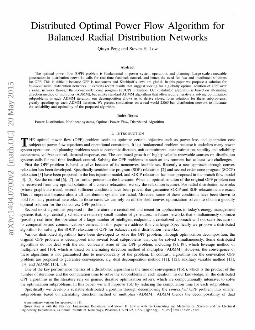
Fig. 1: Notations.

decomposition and superior convergence properties of the method of multipliers [17]. It has broad applications in differentareas and particularly useful when the subproblems can be solved efficiently [18], for example when they admit closed formexpressions, e.g. matrix factorization [19], image recovery [20].

The proposed algorithm has two advantages: 1) There is closed form solution for each optimization subproblem, thuseliminating the need for an iterative procedure to solve a SDP/SOCP problem for each ADMM iteration. 2) Communicationis only required between adjacent buses.

We demonstrate the scalability of the proposed algorithms using a real-life network. In particular, we show that the algorithmconverges within 0.6s for a 2,065-bus system. To show the superiority of deriving close form expression of each subproblems,finally we compare the computation time for solving a subproblem by our algorithm and an off-the-shelf optimization solver(CVX, [21]). Our solver requires on average 6.8 × 10−4s while CVX requires on average 0.5s. On the other hand, we alsoshow that the convergence rate is mainly determined by the diameter 1 of the network through simulating the algorithm ondifferent networks.

The rest of the paper is structured as follows. The OPF problem is defined in section II. In section III, we develop ourdistributed algorithm. In section IV, we test its scalability using data from a real-world distribution network. We conclude thispaper in section V.

II. PROBLEM FORMULATION

In this section, we define the optimal power flow (OPF) problem on a balanced radial distribution network and review howto solve it through SOCP relaxation.

We denote the set of complex numbers with C, the set of n-dimensional complex numbers with Cn. The hermitian transposeof a vector is denoted by ()H . To differentiate vector and scaler operations, the conjugate of a complex scaler is denotedby ()∗. The inner product of two vectors x, y ∈ Cn is denoted by 〈x, y〉 := Re(tr(xHy)). The Euclidean norm of a vectorx ∈ Cn is defined as ‖x‖2 :=

√〈x, x〉.

A. Branch flow model

We model a distribution network by a directed tree graph T := (N , E) where N := {0, . . . , n} represents the set of busesand E represents the set of distribution lines connecting the buses in N . Index the root of the tree by 0 and let N+ := N \{0}denote the other buses. For each node i, it has a unique ancestor Ai and a set of children nodes, denoted by Ci. We adopt thegraph orientation where every line points towards the root. Each directed line connects a node i and its unique ancestor Ai.We hence label the lines by E := {1, . . . , n} where each i ∈ E denotes a line from i to Ai.

For each bus i ∈ N , let Vi = |Vi|eiθi be its complex voltage and vi := |Vi|2 be its magnitude squared. Let si := pi + iqibe its net complex power injection which is generation minus load. For each line i ∈ E , let zi = ri + ixi be its compleximpedance. Let Ii be the complex branch current from bus i to Ai and `i := |Ii|2 be its magnitude squared. Let Si := Pi+ iQibe the branch power flow from bus i to Ai. The notations are illustrated in Fig. 1. A variable without a subscript denotes acolumn vector with appropriate components, as summarized below.

v := (vi, i ∈ N ) s := (si, i ∈ N )` := (`i, i ∈ E) S := (Si, i ∈ E)

Branch flow model is first proposed in [22], [23] for radial network. It has better numerical stability than bus injection modeland has been advocated for the design and operation for radial distribution network, [5], [14], [24]. It ignores the phase anglesof voltages and currents and uses only the set of variables (v, s, `, S). Given a radial network T , the branch flow model is

1The diameter of a graph is defined as the number of hops between two furthest nodes.

3

defined by:

vAi − vi + (ziS∗i + Siz

∗i )− `i|zi|2 = 0 i ∈ E (1a)∑

j∈Ci

(Sj − `jzj) + si − Si = 0 i ∈ N (1b)

|Si|2 = vi`i i ∈ E (1c)

where S0 = 0 ( the root of the tree does not have parent) for ease of presentation. Given a vector (v, s, `, S) that satisfies(1), the phase angles of the voltages and currents can be uniquely determined if the network is a tree. Hence the branch flowmodel (1) is equivalent to a full AC power flow model. See [5, Section III-A] for details.

B. OPF and SOCP relaxationThe OPF problem seeks to optimize certain objective, e.g. total line loss or total generation cost, subject to power flow

equations (1) and various operational constraints. We consider an objective function of the following form:

F (p) =∑i∈N

fi(pi) :=∑i∈N

(αi2p2i + βipi

)(2)

where αi, βi ≥ 0. For instance,• to minimize total line loss, we can set αi = 0 and βi = 1 for each bus i ∈ N .• to minimize generation cost, we can set αi = 0 and βi = 0 for bus i where there is no generator and for generator busi, the corresponding αi, βi depends on the characteristic of the generator.

We consider two operational constraints. First, the power injection si at each bus i is constrained to be in a region Ii, i.e.

si ∈ Ii for i ∈ N (3)

The feasible power injection region Ii is determined by the controllable devices attached to bus i. Some common controllableloads are:• For controllable load, whose real power can vary within [p

i, pi] and reactive power can vary within [q

i, qi], the injection

region Ii is

Ii = {p+ iq | p ∈ [pi, pi], q ∈ [q

i, qi]} ⊆ C (4a)

• For solar panel connecting the grid through a inverter with nameplate si, the injection region Ii is

Ii = {p+ iq | p ≥ 0, p2 + q2 ≤ s2i } ⊆ C (4b)

Second, the voltage magnitude at each bus i ∈ N needs to be maintained within a prescribed region, i.e.

vi ≤ vi ≤ vi for i ∈ N (5)

Typically the voltage magnitude at the substation bus 0 is assumed to be fixed at some prescribed value, i.e. v0 = v0. Atother bus i ∈ N+, the voltage magnitude is typically allowed to deviate by 5% from its nominal value 1, i.e. vi = 0.952 andvi = 1.052.

To summarize, the OPF problem for radial network is

OPF: min∑i∈N

fi(pi)

over v, s, S, ` (6)s.t. (1), (3) and (5)

The OPF problem (6) is nonconvex due to the quadratic equality constraint (1c). In [4], [5], (1c) is relaxed to a secondorder cone constraint:

|Si|2 ≤ vi`i for i ∈ E , (7)

resulting in a second-order cone program (SOCP) relaxation of (6)

ROPF: min∑i∈N

fi(pi)

over v, s, S, ` (8)s.t. (1a), (1b), (7) and (3), (5)

Clearly the relaxation ROPF (8) provides a lower bound for the original OPF problem (6) since the original feasible set isenlarged. The relaxation is called exact if every optimal solution of ROPF attains equality in (1c) and hence is also optimalfor the original OPF. For network with tree topology, SOCP relaxation is exact under some mild conditions [5], [24].

4

III. DISTRIBUTED ALGORITHM FOR OPFWe assume SOCP relaxation is exact and develop in this section a distributed algorithm that solves ROPF. We first review

a standard alternating direction method of multiplier (ADMM). We then make use of the structure of ROPF to speed up thestandard ADMM algorithm by deriving closed form expressions for the optimization subproblems in each ADMM iteration.

A. Preliminary: ADMMADMM blends the decomposability of dual decomposition with the superior convergence properties of the method of

multipliers [17]. For our application, we consider optimization problems of the form:

min f(x) + g(z)

over x ∈ Kx, z ∈ Kz (9)s.t. x = z

where Kx,Kz are convex sets. Let λ denote the Lagrange multiplier for the constraint x = z. Then the augmented Lagrangianis defined as

Lρ(x, z, λ) := f(x) + g(z) + 〈λ, x− z〉+ ρ

2‖x− z‖22, (10)

where ρ ≥ 0 is a constant. When ρ = 0, the augmented Lagrangian reduces to the standard Lagrangian. At each iteration k,ADMM consists of the iterations:

xk+1 ∈ arg minx∈Kx

Lρ(x, zk, λk) (11a)

zk+1 ∈ arg minz∈Kz

Lρ(xk+1, z, λk) (11b)

λk+1 = λk + ρ(xk+1 − zk+1) (11c)

Compared to dual decomposition, ADMM is guaranteed to converge to an optimal solution under less restrictive conditions.Let

rk := ‖xk − zk‖2 (12a)sk := ρ‖zk − zk−1‖2 (12b)

which can be viewed as the residuals for primal and dual feasibility. Assume:• A1: f and g are closed proper and convex.• A2: The unaugmented Lagrangian L0 has a saddle point.

The correctness of ADMM is guaranteed by the following result; see [17, Chapter 3].Proposition 3.1 ( [17]): Suppose A1 and A2 hold. Let p∗ be the optimal objective value. Then

limk→∞

rk = 0, limk→∞

sk = 0

and

limk→∞

f(xk) + g(zk) = p∗

B. Apply ADMM to OPF problemWe assume the SOCP relaxation is exact and now derive a distributed algorithm for solving ROPF (8) that has the following

advantages:• Each bus only needs to solves a local subproblem in each iteration of (11). Moreover there is a closed form solution for

each subproblem, in contrast to most algorithms that employ iterative procedure to solve these subproblems [8]–[15].• Communication is only required between adjacent buses.The ROPF problem defined in (8) can be written explicitly as:

min∑i∈N

fi(pi) (13a)

over v, s, S, ` (13b)

s.t. vAi − vi + ziS∗i + Siz

∗i − `i|zi|2 = 0 i ∈ E (13c)∑

i∈Ci

(Sj − zj`j)− Si + si = 0 i ∈ N (13d)

|Si|2 ≤ vi`i i ∈ E (13e)si ∈ Ii i ∈ N (13f)vi ≤ vi ≤ vi i ∈ N (13g)

5

TABLE I: Multipliers associated with constraints (14g)-(14h)

λ1,i: S(x)i = S

(z)i λ2,i: `

(x)i = `

(z)i

λ3,i: v(x)i = v

(z)i λ4,i: s

(x)i = s

(z)i

µ1,i: S(x)i,Ai

= S(z)i µ2,i: `

(x)i,Ai

= `(z)i

γi: v(x)Ai,i

= v(z)Ai

Assume each bus i is an agent that maintains local variables (vi, si, Si, `i). Then (13e)–(13g) are local constraints to agent(bus) i. (13c) and (13d) describe the coupling constraints among i and its parent Ai and the set of children in Ci, i.e. (13c)models the voltage of its ancestor Ai as a function of the local variables of i, (13d) describes the power flow balance amongthe set of children Ci and bus i itself. To decouple the constraints (13c)–(13d), for each bus i, its ancestor Ai sends its voltagevAi to i, denoted by vAi,i and each child j ∈ Ci sends the branch power to i, denoted by Sj,i and current to i, denoted by`j,i. Then ROPF can be written equivalently as follows.

min∑i∈N

fi(p(z)i ) (14a)

over x := {v(x)i , s(x)i , S

(x)i , `

(x)i , v

(x)Ai,i

, S(x)i,Ai

, `(x)i,Ai

, i ∈ N}

z := {v(z)i , s(z)i , S

(z)i , `

(z)i , i ∈ N}

s.t. v(x)Ai,i− v(x)i + zi

(S(x)i

)∗+ S

(x)i z∗i − `

(x)i |zi|

2 = 0 i ∈ E (14b)∑i∈Ci

(S(x)j,i − zj`

(x)j,i

)− S(x)

i + s(x)i = 0 i ∈ N (14c)

|S(z)i |

2 ≤ v(z)i `(z)i i ∈ E (14d)

s(z)i ∈ Ii i ∈ N (14e)

vi ≤ v(z)i ≤ vi i ∈ N (14f)

S(x)i,Ai

= S(z)i , `

(x)i,Ai

= `(z)i , v

(x)Ai,i

= v(z)Ai

i ∈ N (14g)

S(x)i = S

(z)i , `

(x)i = `

(z)i , v

(x)i = v

(z)i , s

(x)i = s

(z)i i ∈ N (14h)

where (14g) and (14h) are consensus constraints that force all the copies of each variable to be the same. Since ADMM hastwo separate groups of variables x and z that is updated alternatively, we put superscripts (·)(x) and (·)(z) on each variable todenote whether the variable is updated in the x-update or z-update step.

Next, we apply ADMM to decompose (14) by relaxing the consensus constraints in (14g) and (14h). Let λ, µ, γ be theLagrangian multipliers associated with (14g) and (14h) as specified in Table I.

Denote

xi :=(v(x)i , `

(x)i , S

(x)i , s

(x)i

)xj,i :=

(`(x)j,i , S

(x)j,i

)zi :=

(v(z)i , `

(z)i , S

(z)i , s

(z)i

)λi := (λk,i, k = 1, 2, 3, 4)

µi := (µk,i, k = 1, 2)

The variables maintained by each agent (bus) i are its local variables for itself: xi, zi, the copy of its parent’s voltage v(x)Ai,i,

the copy xj,i from each of its child j ∈ Ci and the associated Lagrangian multipliers. Let Ai denote the set of variables, then

Ai := {xi, v(x)Ai,i, {xj,i, µj , j ∈ Ci}, zi, λi, γi}

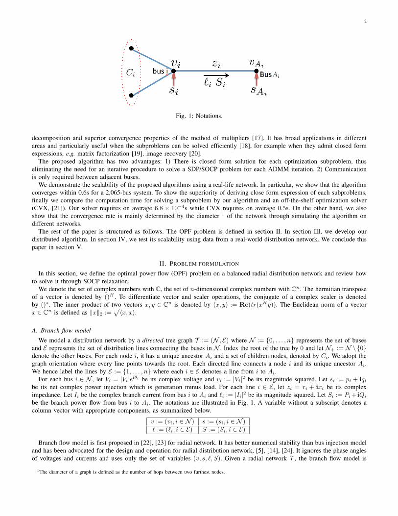
Next, we demonstrate that the problem in (14) can be solved in a distributed manner using ADMM, i.e. both the x-update(11a) and z-update (11b) can be decomposed into small subproblems that can be solved simultaneously by each agent i. Forease of presentation, we remove the iteration number k in (11) for all the variables, which will be updated accordingly aftereach subproblem is solved. The augmented Lagrangian for modified ROPF problem is given in (15). Note that in (15), xi,Aiand zi consist of different components and xi,Ai − zi is composed of the components that appear in both xi,Ai and zi, i.e.xi,Ai − zi :=

(S(x)i,Ai− S(z)

i , `(x)i,Ai− `(z)i

).

6

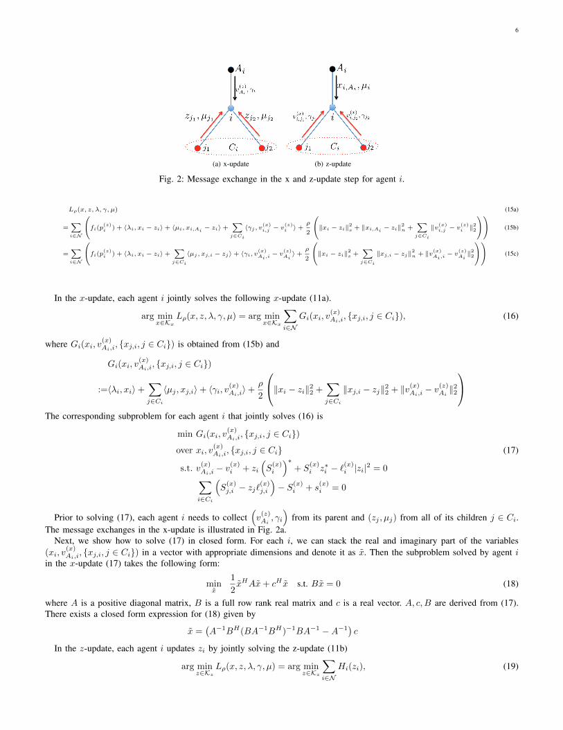
(a) x-update (b) z-update

Fig. 2: Message exchange in the x and z-update step for agent i.

Lρ(x, z, λ, γ, µ) (15a)

=∑i∈N

fi(p(z)i ) + 〈λi, xi − zi〉+ 〈µi, xi,Ai − zi〉+∑j∈Ci

〈γj , v(x)i,j − v(z)i 〉+

ρ

2

‖xi − zi‖2s + ‖xi,Ai − zi‖2n +

∑j∈Ci

‖v(x)i,j − v(z)i ‖

22

(15b)

=∑i∈N

fi(p(z)i ) + 〈λi, xi − zi〉+∑j∈Ci

〈µj , xj,i − zj〉+ 〈γi, v(x)Ai,i− v(z)Ai

〉+ρ

2

‖xi − zi‖2s +∑j∈Ci

‖xj,i − zj‖2n + ‖v(x)Ai,i− v(z)Ai

‖22

(15c)

In the x-update, each agent i jointly solves the following x-update (11a).

arg minx∈Kx

Lρ(x, z, λ, γ, µ) = arg minx∈Kx

∑i∈N

Gi(xi, v(x)Ai,i

, {xj,i, j ∈ Ci}), (16)

where Gi(xi, v(x)Ai,i

, {xj,i, j ∈ Ci}) is obtained from (15b) and

Gi(xi, v(x)Ai,i

, {xj,i, j ∈ Ci})

:=〈λi, xi〉+∑j∈Ci

〈µj , xj,i〉+ 〈γi, v(x)Ai,i〉+ ρ

2

‖xi − zi‖22 + ∑j∈Ci

‖xj,i − zj‖22 + ‖v(x)Ai,i− v(z)Ai

‖22

The corresponding subproblem for each agent i that jointly solves (16) is

min Gi(xi, v(x)Ai,i

, {xj,i, j ∈ Ci})

over xi, v(x)Ai,i

, {xj,i, j ∈ Ci} (17)

s.t. v(x)Ai,i− v(x)i + zi

(S(x)i

)∗+ S

(x)i z∗i − `

(x)i |zi|

2 = 0∑i∈Ci

(S(x)j,i − zj`

(x)j,i

)− S(x)

i + s(x)i = 0

Prior to solving (17), each agent i needs to collect(v(z)Ai, γi

)from its parent and (zj , µj) from all of its children j ∈ Ci.

The message exchanges in the x-update is illustrated in Fig. 2a.Next, we show how to solve (17) in closed form. For each i, we can stack the real and imaginary part of the variables

(xi, v(x)Ai,i

, {xj,i, j ∈ Ci}) in a vector with appropriate dimensions and denote it as x. Then the subproblem solved by agent iin the x-update (17) takes the following form:

minx

1

2xHAx+ cH x s.t. Bx = 0 (18)

where A is a positive diagonal matrix, B is a full row rank real matrix and c is a real vector. A, c,B are derived from (17).There exists a closed form expression for (18) given by

x =(A−1BH(BA−1BH)−1BA−1 −A−1

)c

In the z-update, each agent i updates zi by jointly solving the z-update (11b)

arg minz∈Kz

Lρ(x, z, λ, γ, µ) = arg minz∈Kz

∑i∈N

Hi(zi), (19)

7

where Hi(zi) is obtained from (15c) and

Hi(zi) := fi(p(z)i )− 〈λi, zi〉 − 〈µi, zi〉 −

∑j∈Ci

〈γj , v(z)i 〉+ρ

2

‖xi − zi‖22 + ‖xi,Ai − zi‖22 + ∑j∈Ci

‖v(x)i,j − v(z)i ‖

22

The corresponding subproblem for each agent i that jointly solves (19) is

min Hi(zi)

over zi (20)

s.t. |S(z)i |

2 ≤ v(z)i `(z)i

s(z)i ∈ Iivi ≤ v

(z)i ≤ vi

Prior to solving (20), each agent i needs to collect (xi,Ai , µi) from its parent and (v(x)i,j , γj) from all of its children j ∈ Ci.

The message exchanges in the z-update is illustrated in Fig. 2b.Next, we show how to solve (20) in closed form. Note that

Hi(zi) :=fi(p(z)i )− 〈λi, zi〉 − 〈µi, zi〉 −

∑j∈Ci

〈γj , v(z)i 〉+ρ

2

‖xi − zi‖22 + ‖xi,Ai − zi‖22 + ∑j∈Ci

‖v(x)i,j − v(z)i ‖

22

=ρ

(|S(z)

i − Si|2 + |`(z)i − ˆi|2 +

|Ci|+ 1

2|v(z)i − vi|2

)+ fi(p

(z)i ) +

ρ

2‖s(z)i − si‖

22 + constant (21)

We use square completion to obtain (21) and the variables labeled with hat are some constants. Then (20) can be furthereddecomposed into two subproblems as below. The first one is

min∣∣∣S(z)i − Si

∣∣∣2 + ∣∣∣`(z)i − ˆi

∣∣∣2 + |Ci|+ 1

2

∣∣∣v(z)i − vi∣∣∣2

over v(z)i , `

(z)i , S

(z)i (22)

s.t.∣∣∣S(z)i

∣∣∣2 ≤ v(z)i `(z)i

vi ≤ v(z)i ≤ vi

The optimization problem in (22) has a quadratic objective, a second order cone constraint and a box constraint. We illustratein Appendix A the procedure that solves (22). Compared with using generic iterative solver, the procedure is computationallyefficient since it only requires to solve the zero of three polynomials with degree less than or equal to 4, which have closedform expression.

The second problem is

min fi

(p(z)i

)+ρ

2

∥∥∥s(z)i − si∥∥∥22

over s(z)i (23)

s.t. s(z)i ∈ Ii

Recall that fi(p(z)i

):= αi

2 p2i + βipi as in (2). If Ii takes the form of (4a), the closed form solution to (23) is

p(z)i =

[ρpi − βα+ ρ

]pipi

q(z)i = [qi]

qiqi

where [x]ba := min{a,max{x, b}}. If Ii takes the form of (4b), there also exists a closed form expression to (23) and theprocedure is relegate to Appendix B.

Finally, we specify the initialization and stopping criteria for the algorithm. A good initialization usually reduce the numberof iterations for convergence. We use the following initialization suggested by our empirical results. We first initialize the zvariable. The voltage magnitude square v(z)i = 1. The power injection s(z)i is picked up from a feasible point in the feasibleregion Ii. The branch power S(z)

i is the aggregate power injection s(z)i from the nodes connected by line i (Note that the

network has a tree topology.). The branch current `(z)i =|S(z)i |

2

v(z)i

according to (1c). The x variables are initialized using thecorresponding z variable according to (14g)-(14h). Intuitively, the above initialization procedure can be interpreted as a solutionto the branch flow equation (1) assuming zero impedance on all the lines.

8

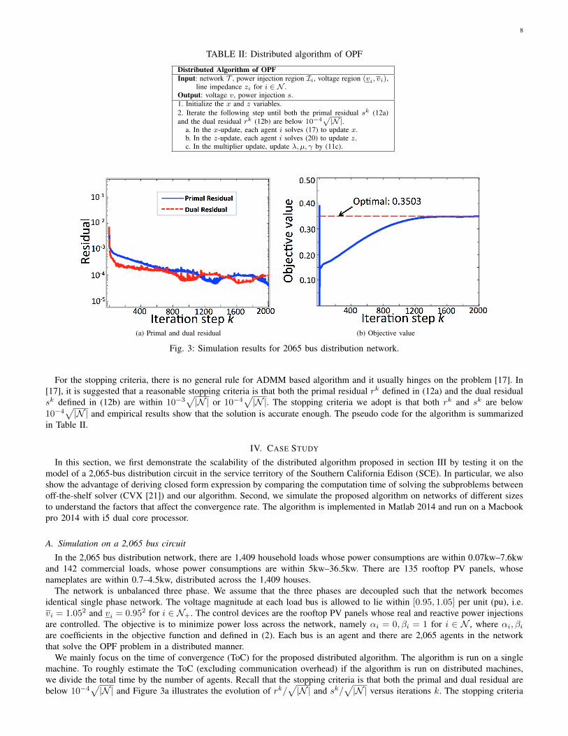
TABLE II: Distributed algorithm of OPF

Distributed Algorithm of OPFInput: network T , power injection region Ii, voltage region (vi, vi),

line impedance zi for i ∈ N .Output: voltage v, power injection s.1. Initialize the x and z variables.2. Iterate the following step until both the primal residual sk (12a)and the dual residual rk (12b) are below 10−4

√|N |.

a. In the x-update, each agent i solves (17) to update x.b. In the z-update, each agent i solves (20) to update z.c. In the multiplier update, update λ, µ, γ by (11c).

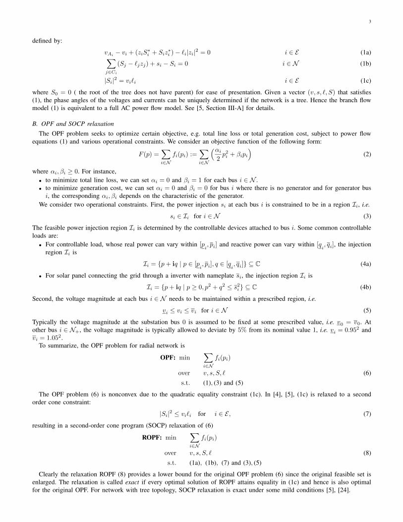
(a) Primal and dual residual (b) Objective value

Fig. 3: Simulation results for 2065 bus distribution network.

For the stopping criteria, there is no general rule for ADMM based algorithm and it usually hinges on the problem [17]. In[17], it is suggested that a reasonable stopping criteria is that both the primal residual rk defined in (12a) and the dual residualsk defined in (12b) are within 10−3

√|N | or 10−4

√|N |. The stopping criteria we adopt is that both rk and sk are below

10−4√|N | and empirical results show that the solution is accurate enough. The pseudo code for the algorithm is summarized

in Table II.

IV. CASE STUDY

In this section, we first demonstrate the scalability of the distributed algorithm proposed in section III by testing it on themodel of a 2,065-bus distribution circuit in the service territory of the Southern California Edison (SCE). In particular, we alsoshow the advantage of deriving closed form expression by comparing the computation time of solving the subproblems betweenoff-the-shelf solver (CVX [21]) and our algorithm. Second, we simulate the proposed algorithm on networks of different sizesto understand the factors that affect the convergence rate. The algorithm is implemented in Matlab 2014 and run on a Macbookpro 2014 with i5 dual core processor.

A. Simulation on a 2,065 bus circuit

In the 2,065 bus distribution network, there are 1,409 household loads whose power consumptions are within 0.07kw–7.6kwand 142 commercial loads, whose power consumptions are within 5kw–36.5kw. There are 135 rooftop PV panels, whosenameplates are within 0.7–4.5kw, distributed across the 1,409 houses.

The network is unbalanced three phase. We assume that the three phases are decoupled such that the network becomesidentical single phase network. The voltage magnitude at each load bus is allowed to lie within [0.95, 1.05] per unit (pu), i.e.vi = 1.052 and vi = 0.952 for i ∈ N+. The control devices are the rooftop PV panels whose real and reactive power injectionsare controlled. The objective is to minimize power loss across the network, namely αi = 0, βi = 1 for i ∈ N , where αi, βiare coefficients in the objective function and defined in (2). Each bus is an agent and there are 2,065 agents in the networkthat solve the OPF problem in a distributed manner.

We mainly focus on the time of convergence (ToC) for the proposed distributed algorithm. The algorithm is run on a singlemachine. To roughly estimate the ToC (excluding communication overhead) if the algorithm is run on distributed machines,we divide the total time by the number of agents. Recall that the stopping criteria is that both the primal and dual residual arebelow 10−4

√|N | and Figure 3a illustrates the evolution of rk/

√|N | and sk/

√|N | versus iterations k. The stopping criteria

9

TABLE III: Statistics of different networks

Network Diameter Iteration Total Time(s) Avg time(s)2065Bus 64 1114 1153 0.561313Bus 53 671 471 0.36792Bus 45 524 226 0.29363Bus 36 289 112 0.24108Bus 16 267 16 0.14

(a) Line network (b) Fat tree network

Fig. 4: Topology for tree and fat tree networks.

are satisfied after 1, 114 iterations. The evolution of the objective value is illustrated in Figure 3b. It takes 1,153s to run 1,114iterations on a single computer. Then the ToC is roughly 0.56s if we implement the algorithm in a distributed manner notcounting communication overhead.

Finally, we show the advantage of closed form solution by comparing the computation time of solving the subproblemsby an off-the-shelf solver (CVX) and by our algorithm. In particular, we compare the average computation time of solvingthe subproblem in both the x-update and the z-update step. In the x-update step, the average time required to solve thesubproblem is 1.7 × 10−4s for the proposed algorithm but 0.2s for CVX. In the z-update step, the average time required tosolve the subproblem is 5.1 × 10−4s for the proposed algorithm but 0.3s for CVX. Thus, each ADMM iteration only takesabout 6.8× 10−4s for the proposed algorithm but 0.5s for using iterative algorithm, which is a 1,000x speedup.

B. Rate of Convergence

In section IV-A, we demonstrate that the proposed distributed algorithm can dramatically reduce the computation time withineach iteration and therefore is scalable to a large practical 2,065 bus distribution network. The time of convergence(ToC) isdetermined by both the computation time required within each iteration and the number of iterations. In this subsection, westudy the number of iterations, namely rate of convergence.

To our best knowledge, most of the works on convergence rate for ADMM based algorithms study how the primal/dualresidual changes as the number of iterations increases. Specifically, it is proved in [25], [26] that the general ADMM basedalgorithms converge linearly under certain assumptions. Here, we consider the rate of convergence from another two factors,network size N and diameter D, i.e. given the termination criteria in Table II, the impact from network size and diameter onthe number of iterations. The impacts from other factors, e.g. form of objective function and constraints, etc. are beyond thescope of this paper.

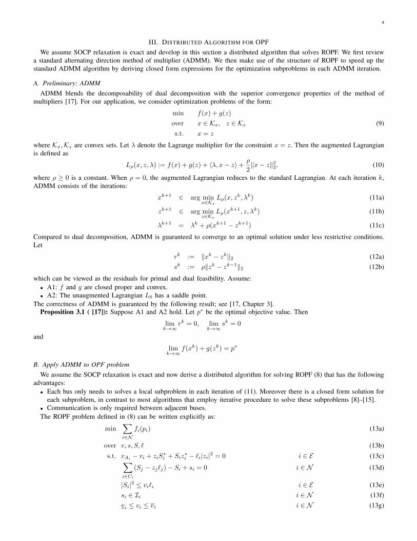
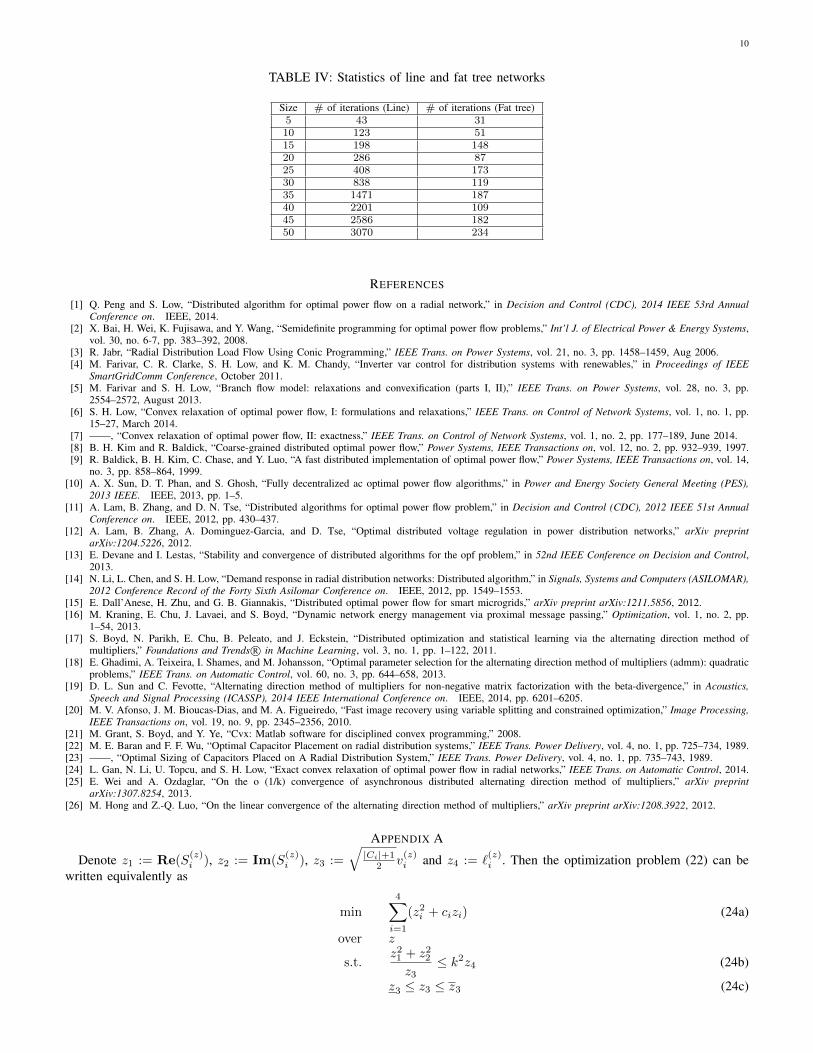
First, we simulate the algorithm on different networks (that are subnetworks of the 2,065-bus system) and some statisticsare given in Table III. For simplicity, we assume the number of iterations T to converge takes the linear form T = aN + bD.Using the data in Table III, the parameters a = 0.34, b = 5.53 give the least square error. It means that the network diameterhas a stronger impact than the network size on the rate of convergence.

To further illustrate the phenomenon, we simulate the algorithm on two extreme cases: 1) Line network in Fig. 4a, whosediameter is the largest given the network size, 2) Fat tree network in Fig. 4b, whose diameter is the smallest (2) given thenetwork size. In Table IV, we record the number of iterations for both line and fat tree network of different sizes. For linenetwork, the number of iterations increases notably as the size increases. For fat tree network, the trend is less obvious comparedto line network.

V. CONCLUSION

In this paper, we have developed a distributed algorithm for optimal power flow problem based on alternating directionmethod of multiplier for balanced radial distribution network. We have derived a closed form solution for the subproblemssolved by each agent thus significantly reducing the computation time. Preliminary simulation shows that the algorithm isscalable to a 2,065-bus system and the optimization subproblem in each ADMM iteration is solved 1,000x faster than genericoptimization solver.

10

TABLE IV: Statistics of line and fat tree networks

Size # of iterations (Line) # of iterations (Fat tree)5 43 3110 123 5115 198 14820 286 8725 408 17330 838 11935 1471 18740 2201 10945 2586 18250 3070 234

REFERENCES

[1] Q. Peng and S. Low, “Distributed algorithm for optimal power flow on a radial network,” in Decision and Control (CDC), 2014 IEEE 53rd AnnualConference on. IEEE, 2014.

[2] X. Bai, H. Wei, K. Fujisawa, and Y. Wang, “Semidefinite programming for optimal power flow problems,” Int’l J. of Electrical Power & Energy Systems,vol. 30, no. 6-7, pp. 383–392, 2008.

[3] R. Jabr, “Radial Distribution Load Flow Using Conic Programming,” IEEE Trans. on Power Systems, vol. 21, no. 3, pp. 1458–1459, Aug 2006.[4] M. Farivar, C. R. Clarke, S. H. Low, and K. M. Chandy, “Inverter var control for distribution systems with renewables,” in Proceedings of IEEE

SmartGridComm Conference, October 2011.[5] M. Farivar and S. H. Low, “Branch flow model: relaxations and convexification (parts I, II),” IEEE Trans. on Power Systems, vol. 28, no. 3, pp.

2554–2572, August 2013.[6] S. H. Low, “Convex relaxation of optimal power flow, I: formulations and relaxations,” IEEE Trans. on Control of Network Systems, vol. 1, no. 1, pp.

15–27, March 2014.[7] ——, “Convex relaxation of optimal power flow, II: exactness,” IEEE Trans. on Control of Network Systems, vol. 1, no. 2, pp. 177–189, June 2014.[8] B. H. Kim and R. Baldick, “Coarse-grained distributed optimal power flow,” Power Systems, IEEE Transactions on, vol. 12, no. 2, pp. 932–939, 1997.[9] R. Baldick, B. H. Kim, C. Chase, and Y. Luo, “A fast distributed implementation of optimal power flow,” Power Systems, IEEE Transactions on, vol. 14,

no. 3, pp. 858–864, 1999.[10] A. X. Sun, D. T. Phan, and S. Ghosh, “Fully decentralized ac optimal power flow algorithms,” in Power and Energy Society General Meeting (PES),

2013 IEEE. IEEE, 2013, pp. 1–5.[11] A. Lam, B. Zhang, and D. N. Tse, “Distributed algorithms for optimal power flow problem,” in Decision and Control (CDC), 2012 IEEE 51st Annual

Conference on. IEEE, 2012, pp. 430–437.[12] A. Lam, B. Zhang, A. Dominguez-Garcia, and D. Tse, “Optimal distributed voltage regulation in power distribution networks,” arXiv preprint

arXiv:1204.5226, 2012.[13] E. Devane and I. Lestas, “Stability and convergence of distributed algorithms for the opf problem,” in 52nd IEEE Conference on Decision and Control,

2013.[14] N. Li, L. Chen, and S. H. Low, “Demand response in radial distribution networks: Distributed algorithm,” in Signals, Systems and Computers (ASILOMAR),

2012 Conference Record of the Forty Sixth Asilomar Conference on. IEEE, 2012, pp. 1549–1553.[15] E. Dall’Anese, H. Zhu, and G. B. Giannakis, “Distributed optimal power flow for smart microgrids,” arXiv preprint arXiv:1211.5856, 2012.[16] M. Kraning, E. Chu, J. Lavaei, and S. Boyd, “Dynamic network energy management via proximal message passing,” Optimization, vol. 1, no. 2, pp.

1–54, 2013.[17] S. Boyd, N. Parikh, E. Chu, B. Peleato, and J. Eckstein, “Distributed optimization and statistical learning via the alternating direction method of

multipliers,” Foundations and Trends R© in Machine Learning, vol. 3, no. 1, pp. 1–122, 2011.[18] E. Ghadimi, A. Teixeira, I. Shames, and M. Johansson, “Optimal parameter selection for the alternating direction method of multipliers (admm): quadratic

problems,” IEEE Trans. on Automatic Control, vol. 60, no. 3, pp. 644–658, 2013.[19] D. L. Sun and C. Fevotte, “Alternating direction method of multipliers for non-negative matrix factorization with the beta-divergence,” in Acoustics,

Speech and Signal Processing (ICASSP), 2014 IEEE International Conference on. IEEE, 2014, pp. 6201–6205.[20] M. V. Afonso, J. M. Bioucas-Dias, and M. A. Figueiredo, “Fast image recovery using variable splitting and constrained optimization,” Image Processing,

IEEE Transactions on, vol. 19, no. 9, pp. 2345–2356, 2010.[21] M. Grant, S. Boyd, and Y. Ye, “Cvx: Matlab software for disciplined convex programming,” 2008.[22] M. E. Baran and F. F. Wu, “Optimal Capacitor Placement on radial distribution systems,” IEEE Trans. Power Delivery, vol. 4, no. 1, pp. 725–734, 1989.[23] ——, “Optimal Sizing of Capacitors Placed on A Radial Distribution System,” IEEE Trans. Power Delivery, vol. 4, no. 1, pp. 735–743, 1989.[24] L. Gan, N. Li, U. Topcu, and S. H. Low, “Exact convex relaxation of optimal power flow in radial networks,” IEEE Trans. on Automatic Control, 2014.[25] E. Wei and A. Ozdaglar, “On the o (1/k) convergence of asynchronous distributed alternating direction method of multipliers,” arXiv preprint

arXiv:1307.8254, 2013.[26] M. Hong and Z.-Q. Luo, “On the linear convergence of the alternating direction method of multipliers,” arXiv preprint arXiv:1208.3922, 2012.

APPENDIX A

Denote z1 := Re(S(z)i ), z2 := Im(S

(z)i ), z3 :=

√|Ci|+1

2 v(z)i and z4 := `

(z)i . Then the optimization problem (22) can be

written equivalently as

min

4∑i=1

(z2i + cizi) (24a)

over z

s.t.z21 + z22z3

≤ k2z4 (24b)

z3 ≤ z3 ≤ z3 (24c)

11

where z3 > z3 > 0 and ci, k are constants that hinges on the constants in (22).Below we will derive a procedure that solves (24). Let µ ≥ 0 denote the Lagrangian multiplier for constraint (24b) and

λ, λ ≥ 0 denote the Lagrangian multipliers for constraint (24c), then the Lagrangian of P1 is

L(z, µ, λ) =

4∑i=1

(z2i + cizi) + µ

(z21 + z22z3

− k2z4)+ λ(z3 − z3)− λ(z3 − z3)

The KKT optimality conditions imply that the optimal solution z∗ together with the multipliers µ∗, λ∗, λ∗

satisfy the followingequations. For ease of notations, we sometimes skip the superscript ? of the variables in the following analysis.

2z1 + c1 + 2µz1z3

= 0 (25a)

2z2 + c2 + 2µz2z3

= 0 (25b)

2z3 + c3 − µz21 + z22z23

+ λ− λ = 0 (25c)

2z4 + c4 − k2µ = 0 (25d)

λ(z3 − z3) = 0 λ ≥ 0 z3 ≤ z3 (25e)λ(z3 − z3) = 0 λ ≥ 0 z3 ≥ z3 (25f)

µ

(z21 + z22z3

− k2z4)

= 0 µ ≥ 0z21 + z22z3

≤ k2z4 (25g)

Lemma A.1: There exists a unique solution (z∗, µ∗, λ∗, λ∗) to (25) if z3 > z3 ≥ 0.

Proof: P1 is feasible since z = (0, 0, z3, 1) satisfies (24b)-(24c). In addition, P1 is a strictly convex optimization problemsince the objective (24a) is a strictly convex function of z and the constraints (24b) and (24c) are also convex. Hence, there existsa unique solution z∗ to P1, which indicates there exists a unique solution (z∗, µ∗, λ∗, λ

∗) to the KKT optimality conditions

(25).Lemma A.1 says that there exists a unique solution to (25), which is also the optima to P1. In the following, we will

solve (25) through enumerating value of the multipliers µ, λ, λ. Specifically, we first assume µ∗ = 0 (Case 1 below), whichis equivalent to assume constraint (24b) is inactive. If there is a feasible solution to (25), it is the unique solution to (25).Otherwise, we assume µ∗ = 0 (Case 2 below), which is equivalent to assume that the equality is obtained at optimality in(24b).

Case 1: If µ = 0, (25) becomes

2z1 + c1 = 0 (26a)2z2 + c2 = 0 (26b)

2z3 + c3 + λ− λ = 0 (26c)2z4 + c4 = 0 (26d)

λ(z3 − z3) = 0 λ ≥ 0 z3 ≤ z3 (26e)λ(z3 − z3) = 0 λ ≥ 0 z3 ≥ z3 (26f)z21 + z22z3

≤ k2z4 (26g)

The solution to (26a)–(26f) ignoring (26g) is

z1 = −c12, z2 = −c2

2, z3 =

[−c3

2

]z3z3

, z4 = −c42

λ = −(2z3 + c3)1{z3=z3}, λ = −(2z3 + c3)1{z3=z3}

and if the solution satisfies (26g), it is the solution to (25). Otherwise, we go to Case 2.

12

Case 2: If µ > 0, (25) becomes

2z1 + c1 + 2µz1z3

= 0 (27a)

2z2 + c2 + 2µz2z3

= 0 (27b)

2z3 + c3 − µz21 + z22z23

+ λ− λ = 0 (27c)

λ(z3 − z3) = 0 λ ≥ 0 z3 ≤ z3 (27d)λ(z3 − z3) = 0 λ ≥ 0 z3 ≥ z3 (27e)

µ =1

k2(2z4 + c4) (27f)

z4 =z21 + z22k2z3

(27g)

Substitute (27g) into (27f), we obtain

µ =1

k2(2z4 + c4) =

2(z21 + z22)

k4z3+c4k2

(28)

Then substituting (27f) into (27a)-(27e), we can write (27) equivalently as

2 +c1z1

+ 4(z21 + z22)

k4z23+

2c4k2z3

= 0 (29a)

2 +c2z2

+ 4(z21 + z22)

k4z23+

2c4k2z3

= 0 (29b)

2 +c3z3− 2

(z21 + z22)2

k4z43− c4

z21 + z22z33

+λ− λz3

= 0 (29c)

λ(z3 − z3) = 0 λ ≥ 0 z3 ≤ z3 (29d)λ(z3 − z3) = 0 λ ≥ 0 z3 ≥ z3 (29e)

where (29a)–(29c) are obtained through dividing both sides of (27a)–(27c) by z1, z2 and z3, respectively. The variables µ, z4can be recovered via (27f) and (27g) after we solve (29).By (29a) and (29b),

c1z1

=c2z2

Denote p := z1c1z3

= z2c2z3

. Then (29) is equivalent to the following equations.

p =z1c1z3

=z2c2z3

(30a)

2 +1

pz3= −

(4(c21 + c22)

k4p2 + 2

c4k2z3

)(30b)

2 +c3z3

=2(c21 + c22)

2

k4p4 +

c4(c21 + c22)

k2p2

z3+λ− λz3

(30c)

λ(z3 − z3) = 0 λ ≥ 0 z3 ≤ z3 (30d)λ(z3 − z3) = 0 λ ≥ 0 z3 ≥ z3 (30e)

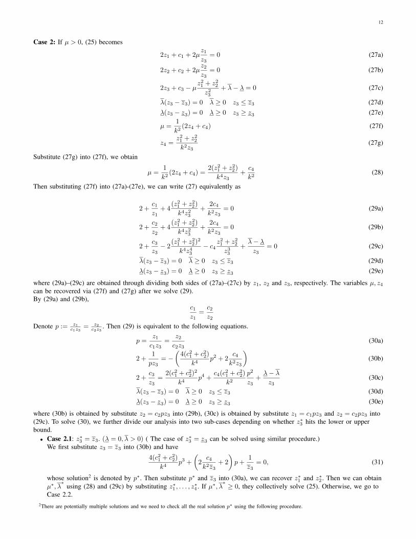
where (30b) is obtained by substitute z2 = c2pz3 into (29b), (30c) is obtained by substitute z1 = c1pz3 and z2 = c2pz3 into(29c). To solve (30), we further divide our analysis into two sub-cases depending on whether z∗3 hits the lower or upperbound.• Case 2.1: z∗3 = z3. (λ = 0, λ > 0) ( The case of z∗3 = z3 can be solved using similar procedure.)

We first substitute z3 = z3 into (30b) and have

4(c21 + c22)

k4p3 +

(2c4k2z3

+ 2

)p+

1

z3= 0, (31)

whose solution2 is denoted by p∗. Then substitute p∗ and z3 into (30a), we can recover z∗1 and z∗2 . Then we can obtainµ∗, λ

∗using (28) and (29c) by substituting z∗1 , . . . , z

∗4 . If µ∗, λ

∗ ≥ 0, they collectively solve (25). Otherwise, we go toCase 2.2.

2There are potentially multiple solutions and we need to check all the real solution p∗ using the following procedure.

13

• Case 2.2: z3 < z∗3 < z3 (λ, λ = 0).Since λ and λ = 0, (30) reduces to

p =z1c1z3

=z2c2z3

(32a)

2 +1

pz3= −

(4(c21 + c22)

k4p2 + 2

c4k2z3

)(32b)

2 +c3z3

=2(c21 + c22)

2

k4p4 +

c4(c21 + c22)

k2p2

z3(32c)

Dividing each side of (32b) by (32c) gives

2z3 +1p

2z3 + c3= − 2

(c21 + c22)p2,

which implies

z3 = − (c21 + c22)p+ 2c32((c21 + c22)p

2 + 2)(33)

Then substitute (33) into (32b), we have

(c21 + c22)p2 + 2

(c21 + c22)p2 + 2c3p

− 2(c21 + c22)

k4p2 +

2c4((c21 + c22)p

2 + 2)

k2((c21 + c22)p+ 2c3)= 1

which is equivalent to

(c21 + c22)2

k4p4 +

c21 + c22k2

(2c3k2− c4

)p3 +

(c3 −

2c4k2

)p− 1 = 0

whose solution is denoted by p∗. Substitute p∗ into (33), we can recover z∗3 , then z∗1 , z∗2 can be recovered via (32a). µ∗ is

recovered using (28). If µ∗ ≥ 0, the corresponding solution solves (25).

APPENDIX B

If Ii takes the form of (4b), the optimization problem (23) takes the following form

minp,q

a12p2 + b1p+

a22q2 + b2q (34a)

s.t. p2 + q2 ≤ c2 (34b)p ≥ 0 (34c)

where a1, a2, c > 0 , b1, b2 are constants. The solutions to (34) are given as below.

Case 1: b1 ≥ 0.

p∗ = 0 q∗ =

[− b2a2

]c−c

Case 2: b1 < 0 and b21a21

+b22a22≤ c2.

p∗ = − b1a1

q∗ = − b2a2

Case 3: b1 < 0 and b21a21

+b22a22> c2.

First solve the following equation in terms of variable λ:

b21(a2 + 2λ)2 + b22(a1 + 2λ)2 = (a1 + 2λ)2(a2 + 2λ)2 (35)

which is a polynomial with degree of 4 and has closed form expression. There are four solutions to (35), but there is onlyone strictly positive λ∗, which can be proved via the KKT conditions of (34). Then we can recover p∗, q∗ from λ∗ using thefollowing equations.

p∗ = − b1a1 + 2λ∗

and q∗ = − b2a2 + 2λ∗

The above procedure to solve (34) is derived from standard applications of the KKT conditions of (34). For brevity, we skipthe proof here.