DYNAMIC MODELING OF VISSIM CRITICAL GAP PARAMETER AT UNSIGNALIZED 1
INTERSECTIONS 2
3
4
5
6
7
Francesco Viti* 8
Faculty of Science, Technology and Communication 9
Research Unit in Engineering Science 10
University of Luxembourg 11
Rue Coudenhove-Kalergi 6, L1359 Luxembourg city, Luxembourg 12
[email protected] 13
14
15
16
Bart Wolput 17 Department of Mechanical Engineering 18
Center for Industrial Management - Traffic and Infrastructure 19
Katholieke Universiteit Leuven 20
Celestijnenlaan 300A - PO Box 2422, 3001 Heverlee, Belgium 21
[email protected] 22
23
24 25
Chris M.J. Tampère 26 Department of Mechanical Engineering 27
Center for Industrial Management - Traffic and Infrastructure 28
Katholieke Universiteit Leuven 29
Celestijnenlaan 300A - PO Box 2422, 3001 Heverlee, Belgium 30
[email protected] 31
32
33
34
35
36
37
38
39
Word Count 40
No. of words: 5100 41
No. of figures: x*250 = 8 Figures, 3 tables 42
Total: 7850 43
44
* Corresponding author, Tel. +352 46 66 44 53 52
ABSTRACT 1
Critical gaps are essential parameters in the modeling of traffic operations at unsignalized intersections and 2
roundabouts, and they are main determinants in the calculation of intersection capacities. In microscopic 3
simulation tools, they are basic vehicle-related variables, and their values and variations among the 4
population are user-defined. Errors or oversimplifications of these basic variables may yield unrealistic 5
results in terms of total throughput, queue lengths, waiting times, etc. 6
In this study we propose a method to calibrate the critical gap parameter in microscopic simulations based 7
on individual travel time observations, and a simple formulation for the calculation of critical gap 8
parameters that takes into account the increasing risk taken by drivers on the minor street with increasing 9
volumes on the major road. This new formulation allows a better match between accepted gaps observed in 10
reality and the actual traffic conditions. 11
The new methodology and model formulation have been used for calibration and validation of the 12
minimum gap parameter of the software program VISSIM using data taken from several unsignalized 13
intersections in the city of Leuven, Belgium. The results show clear outperformance of the volume-14
dependent model with respect to the conventional constant critical gap parameters. 15
16
INTRODUCTION 1
The capacity and service times at minor streets of unsignalized intersections depend on the probability for a 2
vehicle to have sufficient space between vehicles of the higher prioritized streams to pass the conflict areas 3
safely. This probability is function of the vehicle inter-arrival times (or, inversely, the volume or flow rate) 4
on the major streams, as well as it is function of both individual drivers’ and vehicle characteristics, which 5
define each individual gap acceptance behavior. 6
A main difficulty when analyzing gap acceptance behavior at unsignalized intersections is that it mixes 7
drivers’ risk taking behavior and perceptions with the randomness of vehicle inter-arrival times. We can in 8
fact consider the gap acceptance process consisting of two basic elements: 1) the smallest time interval 9
drivers accept when attempting to enter the intersection, so it is driver-dependent; 2) the gap time 10
distribution, which depends on the traffic pattern of the conflicting streams. According to the driver 11
behavior model usually assumed, no driver will enter the intersection unless the gap between vehicles in a 12
higher priority stream is at least equal to the critical gap. In practice, it is not easy to identify the critical 13
gap, as there is no way to measure it directly. This justifies the different definitions and estimation 14
procedures proposed for this parameter. 15
Despite the variety and complexity of operations at unsignalized junctions, conventional models assume a 16
rather simplified gap-acceptance process, based on a characteristic parameter: the minimum or critical gap 17
parameter. This parameter defines the boundary between small and unacceptable gaps, and those gaps 18
considered sufficiently safe. In many capacity models (e.g., in the Highway Capacity Manual, HCM [1]), 19
the critical gap parameter differs only by type of conflict and vehicle operation. Moreover, all drivers are 20
assumed to be homogeneous and generally the gap-acceptance function does not change with time. Gap 21
acceptance models are also adopted in microscopic simulation programs, such as the widely used software 22
VISSIM [2]. In these models the critical gap parameter can change from driver to driver (by specifying 23
different user classes or by drawing the individual parameters from a random distribution), but once the 24
vehicle is loaded in the system it will not change anymore. This assumption, however, does not comply 25
with real driving behavior. Critical gaps do not vary because of differences among drivers only (e.g., age, 26
gender, driving manners, etc.), but additionally, individual drivers have a different tolerance toward risk 27
while waiting in queue that a sufficiently safe gap is available. This risk tolerance, furthermore, depends on 28
the waiting time in queue and then while at the stop-line. Thus the longer a driver waits, the more he is 29
willing to accept risk and the likelihood for accepting shorter gaps increases [3]. 30
An accurate calibration of critical gap parameters has great impact on the validity of simulation results. Too 31
long critical gaps may lead to longer delays and queue lengths than those observed in reality, while too 32
short accepted gaps will result in the opposite behavior and an overestimation of the intersection capacity. 33
The results that can be more easily observed is that a mistake in the calibration of critical gaps will reflect 34
in discrepancy between observed and simulated travel/waiting time distributions. 35
The goal of the research described in this paper is to provide a method to calibrate critical gap functions 36
that are consistent with observed travel times for passing the junction at different traffic conditions. To do 37
so, we propose a new calibration procedure that uses directly simulated and observed travel times, 38
calculated from the moment a vehicle is at the front of the queue until it completes the maneuver. 39
Moreover, we propose a new critical gap function that is traffic flow-dependent. The latter is proposed to 40
capture the changes in risk-taking behavior that drivers show with increasing waiting times in front of the 41
queue due to a reduced chance of acceptable gaps. 42
This paper is outlined as follows. In the next section we provide a state of the art on estimation methods for 43
both unsignalized intersections and roundabouts, and the different definitions of critical gaps proposed, 44
focusing on those used in microsimulation programs. A description of the new estimation methodology 45
follows. Next, data collected from different intersections in the city of Leuven, Belgium, is presented and 46
analyzed, and different critical gap functions are compared when calibrated with this data. The paper is 47
finally concluded with a discussion on the limitations of the current study and a summary of 48
recommendations and further steps in this research direction. 49
STATE-OF-THE-ART 1
Many studies have been conducted on gap acceptance based on the concept of critical gaps, both at 2
unsignalized intersections and at roundabouts. In these studies, different definitions and estimation 3
procedures for the critical gap have been proposed, given the difficulty to measure this parameter directly. 4
The techniques used to estimate critical gap parameters fit into essentially two different groups. The first 5
group is based on regression analysis of the number of drivers that accept a gap against the gap size. If 6
there is a continuous queue on the minor street, then the regression technique produces acceptable results 7
because the output matches the assumptions used in a critical gap analysis. The first empirical studies based 8
on regression analysis proposed different statistical meanings for the critical gap. An early approach 9
suggested by Greenshields et al. [4], used the definition of the “acceptable average minimum time gap” 10
which can be interpreted as a first definition of critical gap. Raff and Hart [5] defined it as the lag for which 11
the number of accepted shorter gaps is equal to the number of rejected longer ones, while analogously 12
Drew [6] suggested that the critical gap is that for which an equal percentage of traffic will accept a smaller 13
gap as will reject a larger one. More recently, Brilon et al. [7] benchmarked different statistical estimation 14
procedures for critical gaps at unsignalized intersections, reporting more than 30 different ways to define 15
and estimate the critical gap parameter, all leading to different capacity calculations. In their study, they 16
argued that critical gaps should not depend on the observed traffic conditions, so that the estimation results 17
can be applied to any unsignalized intersection in undersaturated conditions. 18
It is important to stress out that the regression method can be applied only when there is a queue waiting at 19
the intersection. Only in this case one can be sure that the critical gap and follow up times are independent 20
from the vehicles arrival times. A probabilistic or behavioral approach must be used otherwise. Traditional 21
models of this type are the ones of e.g. Tian et al. [8] and Troutbeck [9]. An exception in this research 22
stream is the work of Wu [10], which is based on the equilibrium between accepted and rejected gaps and 23
does not necessary require a constant waiting queue at the minor street approach. 24
Although simple time and demand independent critical gap parameters based on regression analysis have 25
been adopted in most of the official capacity guides, like in the Highway Capacity Manual [1], simulation 26
models, which are programmed to model traffic operations under different traffic conditions and for 27
different goals, require more refined behavioral models. That explains the development of different models 28
for the gap acceptance behavior (e.g., Mahmassani and Sheffi [11], Daganzo [12] Hewitt [13] and Teply et 29
al. [14-15]). Although many studies such as Teply [14-15] reported a general variation of gap acceptance 30
behavior with traffic conditions and especially on the waiting time for an acceptable gap, they concluded 31
that using this dependence in the modeling of unsignalized intersection would be an unnecessary addition 32
of complexity. 33
Although this call for modeling parsimony may have modeling advantages, it seems counterintuitive given 34
the observed changes in risk attitude of drivers found in other studies, such as Kittelson and Vandehey [16], 35
which found drivers to accept shorter gaps with increased front-queue delays, and Kaysi and Abbany [17], 36
who found statistically significant changes in drivers’ risk-taking behavior with traffic-related parameters 37
such as number of rejected gaps, total waiting time at head of queue, and major-traffic speed. This type of 38
behavior was argued to be relevant when modeling traffic operations, since it may result in lower total 39
delays at the expense of higher risks. Under certain circumstances, drivers from the minor street may 40
decide to take very small gaps, sometimes forcing the drivers from the main street to decelerate and by 41
doing so they can reduce their waiting time at the junction. Capturing this behavior may be relevant if one 42
investigates the safety and operations under dense traffic conditions. Accordingly, modeling of similar 43
types of intersections depends highly on the behavioral characteristics of minor street drivers, and advanced 44
types of models that incorporate aggressive driver attitudes and traffic stream interaction are more 45
appropriate than the basic gap acceptance model. For the same reasons more refined behavioral models that 46
incorporate these changes in the critical gap have been proposed in the last two decades. Cassidy et al. [18] 47
tested different Logit models to estimate the critical gap parameter in simulation programs. They found 48
these models to be highly sensitive to the choice of the critical gap parameter, and recommended adopting 49
different values for different intersection layouts and traffic conditions, in discordance with the earlier 50
recommendations of Brilon et al. [7], and Teply [14-15]. 51
Polus et al. [19-20] focused on the impact of waiting times in the critical gap parameter at roundabout. 52
They reported that such impact causes critical gaps to be significantly lower than the ones suggested by the 53
HCM guide [1]. They recently also suggested to correct this issue using a Logit model with its mean 1
parameter to be a decreasing linear function of the average waiting time [21]. Similarly, Romano [22] used 2
drivers’ delay to determine their tendency to take a risk when entering the main road at a roundabout. In 3
this model the critical gap parameter depends on numerous factors such as the flow on the prioritized 4
stream, the speed of the circulating vehicles, the vehicles mechanical characteristics, the geometry of the 5
entry arms, and the environmental conditions. In analogy with the study presented in this paper, a 6
correlation is found between the critical gap interval and traffic conditions at the roundabout. A model 7
based on the empirical gaps collected on a roundabout in Villaricca (Italy) was used to give a functional 8
form to this correlation. A different microscopic decision model for driver gap-acceptance behavior was 9
proposed by Pollatschek et al. [2]. The model is based on evaluation of the risk associated with not 10
accepting small gaps against the potential benefit of their acceptance, which is the amount of time saved as 11
a result of shorter waiting at the entry line. 12
Although behavioral models have been adopted in simulation to better model traffic operations and for 13
safety analysis, all the above studies have reported significant improvements in the calculation of the 14
intersection capacity, despite the earlier studies striving for parsimony (e.g., [7] and [14-15]) and the 15
recommendations from the official capacity guides (e.g. [1]). For this reason, in this paper we aim to 16
investigate the effect of different traffic loads on the critical gap parameter, and to develop a model that can 17
help improving the results of the widely used microscopic simulation program VISSIM [2] without the 18
need to introduce complex behavioral assumptions to incorporate the change in risk attitude of road drivers. 19
METHODOLOGY 20
Modeling assumptions 21
The total delay experienced by the users at unsignalized intersections consists of two components. A first 22
part of the delay is experienced from the moment they join the back of the queue until they arrive at the 23
queue front, and a second component is the time needed to accept a sufficiently large gap to enter the 24
conflict area. Distinction must be made since the first component depends on the (cumulative) gap 25
acceptance behavior of the users positioned ahead in the queue, as well as on the length of the queue itself, 26
while the second is directly related to users’ (individual) gap acceptance behavior and the traffic flow rate 27
at the major traffic stream. The focus of this paper is on the calibration of the critical gap parameter so the 28
main contribution of this study is the development of a calibration procedure that does not consider the 29
effect of delays while in queue but only those while waiting for an acceptable gap. 30
In the software program VISSIM, depending on the traffic conditions each vehicle has two basic conditions 31
in its gap-acceptance behavior: 32
- Minimum headway (distance) 33
- Minimum (critical) gap time 34
As rule of thumb, for the free flow traffic on the main road the minimum gap time is the relevant condition. 35
For slow moving or queuing traffic on the main road the minimum headway becomes the most relevant 36
condition. In this paper we consider only low-dense traffic conditions on the major street. 37
The critical gap time as defined in this paper follows the definition given in VISSIM, which is different 38
from the critical gap time specified for instance in the Highway Capacity Manual. Essentially, the HCM 39
measures the gap time from the rear of the last vehicle that has passed the junction and the front of the next 40
vehicle arriving at the intersection in the major stream. In VISSIM the priority rule is instead regulated by 41
the distance between the front of the vehicle arriving and the beginning of the intersection. The difference 42
is therefore dependent on the size of the intersection and the mean speed on the major stream. In general, 43
the values provided by the HCM are systematically higher than those given in this paper. 44
To analyze the effect of traffic conditions on the critical gap, we here identify concurrent reasons for 45
observing differences in drivers’ gap acceptance behavior. Some factors that affect this behavior are [23]: 46
- Factors related to the infrastructure 47
o type of conflict/movement 48
o slope 49
o number of lanes 50
o intersection layout 1
o speed limits 2
- Traffic related factors 3
o percentage of heavy traffic 4
o mean speed on the major stream 5
o inter-arrival distribution 6
o presence of protected flows (cyclists, pedestrians,…) 7
- External factors 8
o weather conditions 9
o visibility 10
- driver related factors 11
o gender 12
o age 13
o aggressiveness 14
o perception heterogeneity 15
o compliance to driving rules 16
o perception of danger 17
o purpose of trip 18
o presence of passengers. 19
20
While infrastructural, traffic and external factors can be objectively observed during the data collection 21
process most of the driver-related factors remain unknown. This will also be the case in this study. 22
Estimation procedure 23
The developed estimation procedure is based on a ‘basic unsignalized intersection’, which consists of a T-24
shaped intersection such as in Figure 1 and on travel time measurements instead of the more conventional 25
vehicle inter-arrival times. The travel time measurements used are the times needed for the minor street 26
vehicles to enter the major street. The calibration parameter in this procedure is the critical gap parameter 27
and its variation depends on the demand observed on the major street and the one on the minor street, 28
which are used as input in the VISSIM simulation program, together with the (observed) average traffic 29
composition and the relevant infrastructure-related factors (e.g. speed limit, slope, etc.). 30
31
Figure 1: Basic unsignalized intersection and travel time measurements defined in this study. 32
Travel times are recorded from the yield-sign until the vehicle entering from the minor street has reached a 33
fixed location downstream of the main road. This location was chosen at different distances from the 34
junction to make sure that vehicles merging into the major stream had completed the acceleration phase. 35
In the proposed estimation procedure the distribution of travel times is the key performance measure. This 36
of course has a direct relationship with the traffic conditions on the main street: the higher the flow rate, the 37
longer waiting times will be expected and therefore the longer travel times from the front of the queue to 38
some point downstream of the junction. The choice of the waiting time parameter is in line with research 39
done on roundabouts and described in the previous section [20-22]. 40
Description of the basic cases 41
The case studies have been accurately chosen to control the impact of the factors listed in the methodology 42
section. More specifically we made these choices on the basis of the following characteristics: 43
- T-shaped intersections, to guarantee always one conflict point; 1
- small impact of non-motorized traffic (pedestrians, bicycles, etc.); 2
- no signalized intersections in the neighborhood, which could create regular gaps for the drivers, 3
platooning effects, etc. 4
- single lane approaches, to avoid drivers competing for the available gaps; 5
- clear visibility; 6
- different traffic conditions (i.e. traffic intensities) 7
8
On the basis of these characteristics we have identified five different unsignalized intersections in the area 9
of Leuven, Belgium (See also Table 1 for the specifications of the traffic characteristics of each case): 10
1. Case 1: Blijde Inkomstraat - Herbert Hooverplein –traffic on minor road turns left to join the main 11
street, which is one-way; low presence of heavy vehicles and speed limit of 30km/h on both roads; 12
2. Case 2: Westlaan – Wilgenstraat –traffic on the minor road turns right to join the main street, 13
which is one-way; similar conditions as above, but with higher flows on the main street; 14
3. Case 3: Bondgenotenlaan – Justus Lipsiusstraat –similar as case 1 but with significantly high share 15
of heavy loaded vehicles; 16
4. Case 4: Naamsestraat – Parkstraat –similar as case 2 but with a positive slope on the minor street; 17
5. Case 5: Naamsesteenweg – Koning Leopold III-laan - traffic on the minor road turns right to join 18
the main street, which is a two-way road; speed limit is here fixed to 50 km/h. 19
Data collection strategy 20
To guarantee a correct interpretation of the results and comparison with the VISSIM simulations it is 21
important to collect the data both in real life and in the simulations in the same way. 22
The real measurements consist of two types: we collected the volumes from the major and the minor 23
streams, including also the share of light and heavy duty vehicles and we measured each individual travel 24
time of the vehicles in the minor stream. This operation was done manually using a chronograph. 25
To guarantee a relatively small impact of external factors we collected the data on days with stable good 26
weather and during working days only. All measured data have been collected with a 0.1s accuracy. 27
VISSIM simulations 28
We used the same infrastructure layouts, traffic rules, as well as volumes, mean speeds and percentage of 29
light and heavy duty vehicles in VISSIM. We defined four types of vehicles in the simulations, i.e. cars, 30
vans, busses and trucks. Vehicle lengths, speed and acceleration profiles of each type were chosen 31
according to the default parameters suggested by the program developers. To obtain reliable results we also 32
used ten different random seeds in the simulation program for simulating different random arrivals at the 33
intersection. The minimum gap times modeled were also varying from driver to driver according to a 34
Normal distribution. The distribution interval of gap times utilized was tested to be at the 95% significance 35
level similar to the one measured in reality. 36
Analysis of results 37
Table 1 gives an overview of the data collected at the 5 locations listed above. 38
Table 1: overview of recorded data 39
Case 1 Case 2 Case 3 Case 4 Case 5
Collection time (minutes) 480 120 120 180 180
Mean intensity (veh/h) 258 496 230 252 242
Recorded speeds (km/h) 25-30 25-30 25-30 25-30 40-45
Light duty vehicles (%) 2.9 2.1 3.9 2.0 2.3
Heavy duty vehicles (%) 0.9 1.4 22.4 3.4 4.3
# vehicle records 487 74 244 34 138
In this case more than 80% of the recorded travel times was less than 5 seconds, as it is shown later in 1
Figure 3. The first case was characterized by the longest collection time period. We subdivided this data 2
into 48 time periods of 10 minutes where we assumed stationary traffic conditions (Figure 2). These 3
intervals where then aggregated into four sub-periods with a characteristic mean volume, which was later 4
used as input to perform the VISSIM simulations. 5
6
Figure 2: subdivision of the collection time period of the first case study into four sub-periods. 7
Figure 3 gives an indication of how the VISSIM simulations reproduced realistic travel times in the first 8
case. We operated the same technique also for the other cases. The second case differed significantly from 9
the first one only for a higher volumes recorded during the study period. We therefore aggregated the 10
results, resulting in the relationship between accepted gap times and traffic volumes as shown in Figure 4. 11
12
Figure 3: real data vs. simulated travel times for the first case. 13
Regarding cases 3 to 5 we reported a significant increase of accepted average gap times due to a higher 14
share of heavy loaded vehicles (around 1.5s longer gaps needed on average), no increase in the case of 15
positive slope (about 5.5% maximum slope), and about 1.0s longer gaps in the fifth case, where the mean 16
recorded speeds are higher. 17
Analysis of minimum gap times 18
Figure 4 displays the interval of gap times calibrated on the first two case studies (the middle interval 19
represents the average of the first case over the whole time period). Recall that the goal was to minimize 20
the difference between estimated and observed individual travel times, as shown in Figure 3 so these values 21
100
150
200
250
300
350
400
0 10 20 30 40
de
nsi
ty [
veh
/h]
Measurement interval
Volume on the main stream
Series1
Series2
obserations
mean values
0
5
10
15
20
25
0 20 40 60 80 100
Travel Time [s]
Percentage of the data [%]
Distribution of travel times
Reality
Simulation
represent the intervals of assigned critical gap parameters that minimize the difference between observed 1
and simulated travel times, such as in Figure 3. Figure 4 suggests that the observed gap times tend to get 2
smaller with increasing volumes. This is intuitive given the lower chance for the drivers to find acceptable 3
gaps, and in line with earlier studies on roundabouts (e.g., [19-22]). 4
5
Figure 4: relationship between traffic intensity and accepted gap times for cases 1 and 2. 6
To further investigate this trend we have performed different simulations in VISSIM using different 7
functional forms for the critical gap parameter (Figure 5). More specifically we have analyzed the results 8
when using the constant default parameter suggested by the VISSIM developers, the one used commonly in 9
Belgium (Constant Model 1) and the one found as best calibration of a constant model using all data at 10
once (Constant Model 2), as well as a linearly decreasing model and two different exponential models. 11
12
Figure 5: different functional forms analyzed for the critical gap [24]. 13
To test the goodness of fit we have used different metrics. Table 2 shows the results in terms of average 14
error, its normalized value (Root Mean Squared Error) and the standard deviation. The results of the 15
exponential model are found by calibrating the parameters of the following function: 16
GT = tmin + (tmax – tmin) * exp(-α * (I – I0)) 17
18
where 19
tmax = tbasis + tc,HV * PHV + tc,G * G + tc,S * S / 5 + tc,C; 20
tmin = 0,75 * tmax; 21
α = 0,025; 22
I = intensity (veh/h); 23
2,0
2,5
3,0
3,5
4,0
0 100 200 300 400 500 600
Min
imu
m g
ap t
ime
[s]
Volume [veh/h]
Functional forms used to model the minimum gap times
PTV Default
Tritel Model
Constant Model
Linear Model
Exponential Model 1
Exponential Model 2
Constant Model 1
Constant Model 2
I0 = 240 vtg/h (start of exponential behavior); 1
tbasis = 3,23 s; 2
tc,HV = 0,07 s (correction factor for heavy traffic); 3
PHV = heavy traffic (percentage); 4
tc,G = 0,10 s (correction factor for slope); 5
G = rising slope (percentage); 6
tc,S = 0,23 s (correction factor for speed); 7
S = speed in km/h faster (+) or slower (-) than speed profile 25-30 km/h; 8
tc,C = correction factor for conflict type based on HCM. 9
10
Table 2: results of the calibration of the different models. 11
Constant Model Linear Model Exponential 1 Exponential 2 12
Average error 0.27 0.21 0.19 0.12 13
Error percentage (RMSE%) 7% 6% 5% 3% 14
St. Deviation 0.34 0.27 0.26 0.14 15
16
The result of the calibration is shown graphically in Figure 6. The proposed exponential model is compared 17
with the result of the optimally calibrated constant model but for different mean volumes, and the calibrated 18
linear model. We would stress that the represented 6 points are based on extensive data collection (more 19
than 1000 individual travel times), and they simply represent the averages of similar demand levels from 20
different intersections. 21
22
23
Figure 6: calibration of the proposed exponential model. 24
To assess the validity of the calibrated VISSIM parameter and to compare the goodness of fit of the 25
different parametric curves we checked the robustness of the parameter values with respect to the reliability 26
interval, which is defined as the interval between which 90% of the minimum gap time values lie (5%-95% 27
range). All simulated minimum gap times in VISSIM using the exponential model lie into the reliability 28
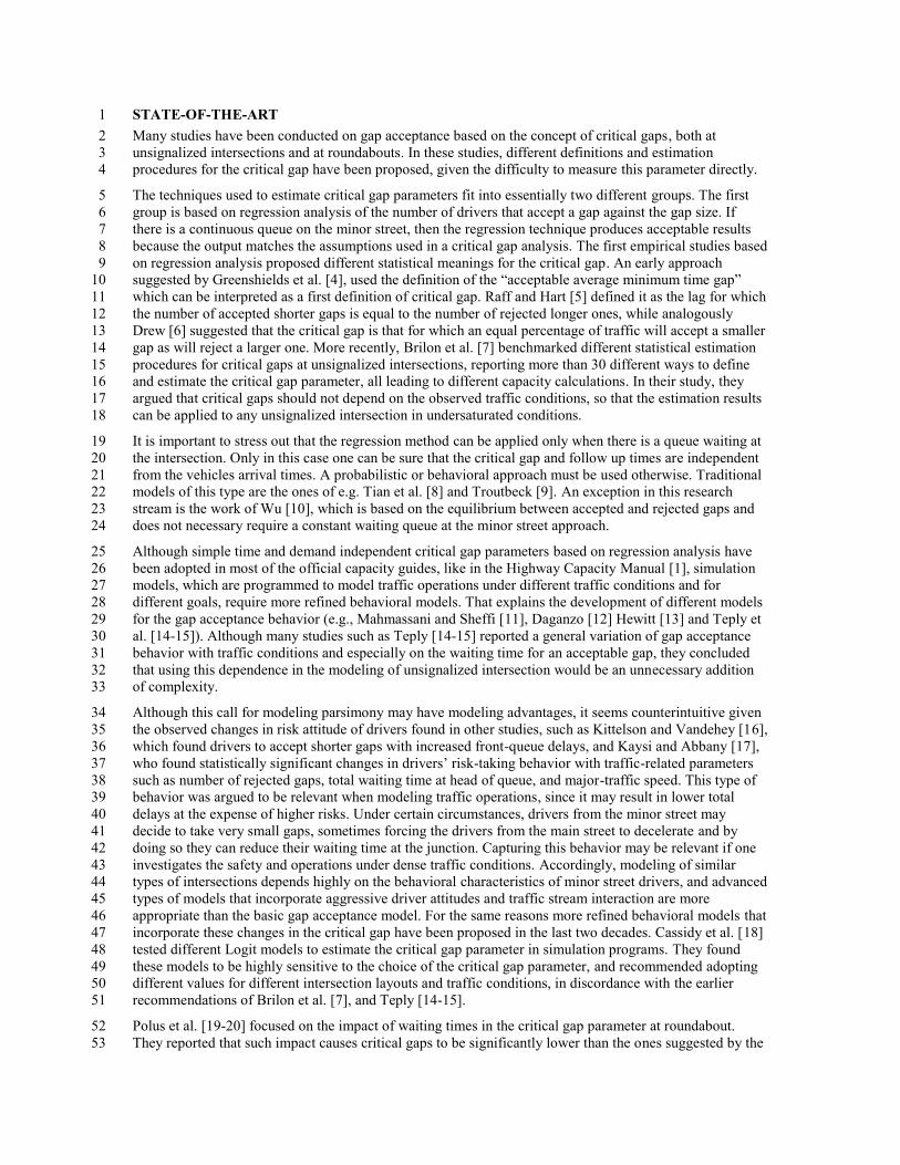
intervals, as shown in Figure 7. This is not the case if the other functional forms are used [24]. Note that, in 29
the picture, the five different cases have been divided into 11 different datasets of homogeneous volumes: 30
1) Case 1 (199 vtg/h); 31
3,4
3,517
3,084
2,821 2,807
2,686
1,5
2,0
2,5
3,0
3,5
4,0
0 100 200 300 400 500 600
Min
imu
m G
ap T
ime
s (s
)
Mean traffic volume [veh/h]
Series1
Series2
Linear (Series2)
Calibrated const. model
Calibrated exp model
Linear Model
2) Case 1 (251 vtg/h); 1
3) Case 1 (258 vtg/h); 2
4) Case 1 (275 vtg/h); 3
5) Case 1 (313 vtg/h); 4
6) Case 2 (496 vtg/h); 5
7) Case 3 (198 vtg/h); 6
8) Case 3 (230 vtg/h); 7
9) Case 3 (274 vtg/h); 8
10) Case 4 (252 vtg/h); 9
11) Case 5 (242 vtg/h). 10
11
12
Figure 7: reliability intervals and results of the proposed exponential model. 13
Model validation 14
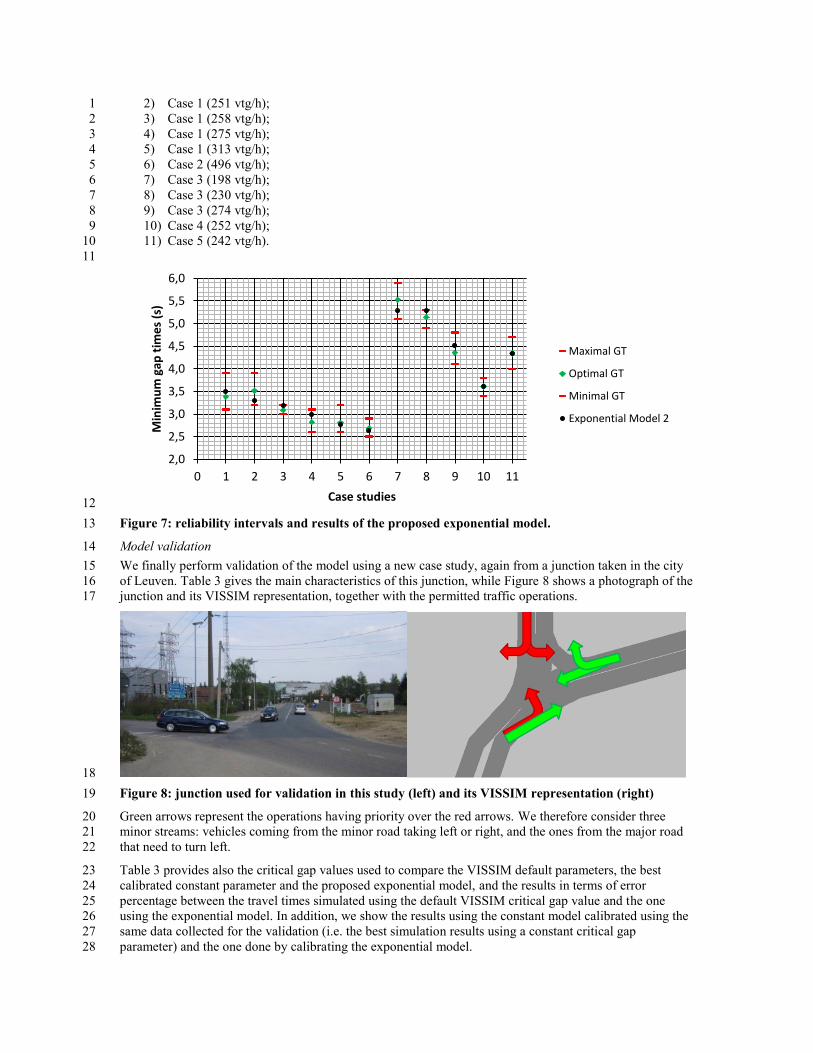
We finally perform validation of the model using a new case study, again from a junction taken in the city 15
of Leuven. Table 3 gives the main characteristics of this junction, while Figure 8 shows a photograph of the 16
junction and its VISSIM representation, together with the permitted traffic operations. 17
18
Figure 8: junction used for validation in this study (left) and its VISSIM representation (right) 19
Green arrows represent the operations having priority over the red arrows. We therefore consider three 20
minor streams: vehicles coming from the minor road taking left or right, and the ones from the major road 21
that need to turn left. 22
Table 3 provides also the critical gap values used to compare the VISSIM default parameters, the best 23
calibrated constant parameter and the proposed exponential model, and the results in terms of error 24
percentage between the travel times simulated using the default VISSIM critical gap value and the one 25
using the exponential model. In addition, we show the results using the constant model calibrated using the 26
same data collected for the validation (i.e. the best simulation results using a constant critical gap 27
parameter) and the one done by calibrating the exponential model. 28
2,0
2,5
3,0
3,5
4,0
4,5
5,0
5,5
6,0
0 1 2 3 4 5 6 7 8 9 10 11
Min
imu
m g
ap t
ime
s (s
)
Case studies
Maximal GT
Optimal GT
Minimal GT
Exponential Model 2
Table 3: main characteristics of the road junction and observed turnings, minimum gap times used 1
in the validation and results of the validation in terms of travel times 2
Northbound Southbound
Data collection time (min) 120 120
Average intensity (veh/h) 207 235
Speed limit (km/h) 50 50
Light duty vehicles (%) 1.7% 2.1%
Heavy duty and buses (%) 1.0% 0.4%
Operation Right turning Left turning Left turning
# of observed vehicles 112 106 84
3
Gap time (s) Right from minor Left from minor Left from major
Default VISSIM 3.0 3.0 3.0
Calibrated constant model 3.4 3.4 3.4
Exponential model 4.2 4.4 2.1
4
Travel time (s) Right from minor Left from minor Left from major Total
Average travel time 4.4 error % 6.9 error % 3.8 error % error %
Default VISSIM 3.93 11% 5.95 14% 3.24 15% 13%
Calibrated constant model 4.25 3% 7.61 10% 3.38 11% 8%
Exponential model 4.61 5% 7.20 4% 2.82 26% 10%
Calibrated exponential model 4.64 5% 7.17 4% 3.28 14% 7%
5
As one can see from Table 3, the exponential model performs very well when applied to the turning 6
operations from the minor street. Results from the exponential model set using the proposed exponential 7
function GT are very close to the best constant model for the minor street vehicles, while they are less 8
accurate for the major stream vehicles. This trend is however shown also for the best calibrated models, 9
pointing at a larger discrepancy between reality and the type of operation simulated with VISSIM. Note 10
that the values in Table 3 are simply an average over a certain distribution that the program VISSIM uses to 11
draw the individual critical gaps. The result of loading critical gaps from this distribution is similar to the 12
distribution of travel times represented in Figure 3, thus accurately mimics the real observations. 13
LIMITATIONS OF THE STUDY AND FURTHER RESEARCH DIRECTIONS 14
Despite the very promising results shown in the validation section, we are aware that the current dataset 15
used to calibrate the models may not reflect all traffic conditions at unsignalized intersections. The 16
calibration of the exponential model parameters is quite well fitting, as shown with Figures 7 and 8, and the 17
form of the exponential model is intuitive, since one can expect that the users start accepting shorter gap 18
times only above a certain traffic load, which may yields to long expected waiting times. However, more 19
data may suggest other functional forms, like the S-shaped function suggested by Polus et al. [25]. 20
The methodology adopted is rather general. However, the results of the calibration are not, and the values 21
found in this paper may differ significantly from case to case. The choice of the T-junctions has facilitated 22
the calibration process significantly. Different conflict points may induce different behavior for the drivers, 23
and this may affect the gap parameter values, as well as different factors not included in the study, will 1
have a significant influence, for instance when the visibility is very different from the T-junctions used (left 2
turning from major roads or merging operations with very sharp angles). Further analysis under different 3
conditions and to identify relevant external factors is needed since all conditions considered where with 4
reasonably good weather and visibility. Also analysis on roundabouts may show some differences, 5
especially if one considers the introduction of the circulating flow parameter. 6
It must also be pointed out that a very important goal for the gap acceptance model is to reproduce well 7
delays and queue lengths observed at minor streets. However, the focus of this study is on the critical gap 8
parameter, its distribution over the population and its variation with different loads on the major street. This 9
is also equally important since critical gap is a main determinant of the intersection capacity and is one of 10
the input parameters that affect gap acceptance behavior. Without a reliable estimation of this parameter, 11
delays and queue length will certainly be erroneously estimated. 12
For the calibration procedure, total individual delays and queue lengths from the minor street could also be 13
used in our framework. However, using the whole individual delay in the process (i.e. from the moment the 14
vehicle joins the queue until it leaves it and merges the main stream) would introduce much more 15
complications and probably reduce the estimation capabilities of the methodology. To give just a few 16
reasons, the full individual delay would include, and be influenced by, the behavior of the other drivers 17
preceding the vehicle. It would be very difficult to extract the correlation in this data type. Moreover, the 18
estimation results would strongly depend on the queue lengths. These are measures that have relatively 19
weaker influence on the critical gap parameter. The word ‘relatively’ is used on purpose since we expect 20
that drivers joining long queues and experiencing long delays before arriving at the front of the queue may 21
show a stronger risk-taking behavior due to loss of time and patience. This effect is partly considered in our 22
method by considering the minimum gap parameters as function of the traffic load on the major stream. 23
Finally, this paper has focused only on the critical gap parameter, while no regard was given to the analysis, 24
calibration and validation of follow up time parameters. The data collected was insufficient to obtain 25
reasonable results and this will be certainly a direction to undertake in future research. 26
SUMMARY AND RECOMMENDATIONS 27
Critical gaps are essential parameters in the modeling of traffic operations at unsignalized intersections. 28
These parameters are also fundamental in simulation studies, which are normally based on gap-acceptance 29
theory. In this paper we have developed and tested on different real cases a new methodology based on 30
individual waiting times at the minor streets to calibrate the minimum gap parameter of a well-known 31
microscopic simulation program, VISSIM. We showed also that significant improvements could be 32
achieved if the simple constant critical gap parameter used in the standard driver model of VISSIM is 33
replaced by a more refined model that is sensitive to the traffic load on the major road. This is in line with 34
past research, who has found evidence of the decreasing average gaps accepted by the drivers with 35
increasing (expected) waiting times. 36
The values found for five different intersections in Leuven, Belgium, and under 11 different scenarios 37
depending on the specific traffic conditions and compositions has been validated also on an intersection in 38
the same area. The results show that the proposed traffic-dependent exponential model outperforms the 39
simpler constant and linear models. Naturally, the better fitting is done at the expense of extra parameters to 40
calibrate, but the advantage for better estimating capacities at unsignalized intersections or safety and 41
operations under dense traffic conditions supports this choice. 42
ACKNOWLEDGEMENTS 43
The authors would like to thank Pieter Vandervelden, whose Master Thesis has largely contributed to this 44
paper, and Katia Organe and Leen De Valck from the Flemish Traffic Center for their support during the 45
editing of the thesis. We also thank the anonymous reviewers for their useful comments. 46
REFERENCES 47
[1] Transportation Research Board (2000). Highway Capacity Manual. Report n. 209, Washington D.C. 48
[2] PTV (2010). VISSIM 5.0 Manual. Karlsrhue, Germany. 49
[3] Pollatschek M.A., Polus A., Livneh M. (2002). A decision model for gap acceptance and capacity at 1
intersections. Transportation Research Part B 36, pp. 649–663. 2
[4] Greenshields, B.D., Shapiro, D., Erickson, E.L., 1947. Traffic performance at urban street 3
intersections. Technical Report 1, Bureau of Highway Traffic, Yale University, New Haven, CT. 4
[5] Raff M. S., Hart, J. W., (1950). A volume warrant for urban stop signs. Eno foundation for highway 5
traffic control: Saugatuck, Connecticut. 6
[6] Drew, D.R. (1968). Traffic Flow Theory and Control. McGraw-Hill Book Company, New York. 7
[7] Brilon W., Koenig R., Troutbeck R.J. (1999). Useful estimation procedures for critical gaps. 8
Transportation Research Part A 33, pp. 161-186. 9
[8] Tian Z.Z., Vandehey M., Bruce W. R., (1999). Implementing the maximum likelihood methodology to 10
measure a driver’s critical gap. Transportation Research Part A 33(3-4), pp. 187–197. 11
[9] Troutbeck R. J. (1992). Estimating the Critical Acceptance Gap from Traffic Movements, Physical 12
Infrastructure Center Report, Queensland University of Technology, Australia. 13
[10] Wu N. (2006). A new model for estimating critical gap and its distribution at unsignalized intersections 14
based on the equilibrium of probabilities. In: Proceeding of the 5th International Symposium on 15
Highway Capacity and Quality of Service. Yokohama, Japan, July 25 - 29, 2006. 16
[11] Mahmassani and Sheffi (1981) Using gap sequences to estimate gap acceptance functions. 17
Transportation Research Part B 15, pp. 143-148. 18
[12] Daganzo (1981). Estimation of gap acceptance parameters within and across the population from direct 19
roadside observation. Transportation Research Part B 15, pp. 1-15. 20
[13] Hewitt, R. H., 1983. Measuring critical gap. Transportation Science 17(1), pp. 87-109. 21
[14] Teply, S., Abou-Henaidy, M.I. and Hunt, J.D. (1997a). Gap acceptance behavior – aggregate and Logit 22
perspectives: Part 1. Traffic Engineering and Control 38(9), pp. 474-82. 23
[15] Teply, S., Abou-Henaidy, M.I. and Hunt, J.D. (1997b). Gap acceptance behavior – aggregate and Logit 24
perspectives: Part 2. Traffic Engineering and Control 38(10), pp. 540-4. 25
[16] Kittelson W.K., Vandehey M.A. (1991). Delay effects on driver gap acceptance characteristics at two-26
way stop-controlled intersections. Transportation Research Records 1320, pp. 154-159. 27
[17] Kaysi I.A., Abbany A.S. (2007). Modeling aggressive driver behavior at unsignalized intersections. 28
Accident Analysis and Prevention 39, pp. 671–678. 29
[18] Cassidy M.J., Madanat S.M., Wang M.-H., Yang F. (1995). Unsignalized intersection capacity and 30
level of service: revisiting critical gap (with discussion and closure). Transportation Research Record 31
1484, pp. 16-23. 32
[19] Polus, A., J. Craus, and I. Reshetnik (1996). Non-stationary gap acceptance assuming drivers’ learning 33
and impatience, Traffic Engineering and Control 37(6), pp. 395-402. 34
[20] Polus, A., Shmueli-Lazar S. (1999), Entry capacity of roundabouts and impact of waiting times. Road 35
and Transport Research 8(3), pp. 43-54. 36
[21] Polus A., Shiftan Y, Shmueli-Lazar S. (2005). Evaluation of the waiting-time effect on critical gaps at 37
roundabouts by a Logit model. European Journal of Transport Infrastructure Research 5(1), pp. 1-12. 38
[22] Romano E. (2005). Modeling Drivers’ Roundabout Behavior. Proceedings of the SIIV Conference, 39
Bari, Italy. 40
[23] Tupper, S. (2010). Initial findings on unsignalized t-intersections, research conducted at the University 41
of Massachusetts. Revisiting Gap Acceptance. Vancouver. 42
[24] Vandervelden P. Dynamische Modellering van Gap Acceptance bij Voorrangskruispunten (Dynamic 43
modeling of gap acceptance at unsignalized intersections, in Flemish). MSc Thesis, Katholieke 44
Universiteit Leuven, Leuven, Belgium. 45
[25] Polus A., Shmueli-Lazar S., Livneh M. (2003). Critical Gap as a Function of Waiting Time in 46
Determining Roundabout Capacity. Journal of Transportation Engineering, Vol. 129(5), pp. 504-509. 47