70
1 EKT 441 MICROWAVE COMMUNICATIONS CHAPTER 4: MICROWAVE FILTERS
| Date post: | 14-Dec-2015 |
| Category: |
Documents |
| Upload: | anabel-haylett |
| View: | 273 times |
| Download: | 12 times |

1
EKT 441MICROWAVE COMMUNICATIONS
CHAPTER 4:
MICROWAVE FILTERS

2
INTRODUCTION
What is a Microwave filter ? linear 2-port network controls the frequency response at a certain point in
a microwave system provides perfect transmission of signal for
frequencies in a certain passband region infinite attenuation for frequencies in the stopband
region a linear phase response in the passband (to reduce
signal distortion).f2

3
INTRODUCTION
The goal of filter design is to approximate the ideal requirements within acceptable tolerance with circuits or systems consisting of real components.
f1
f3
f2
Commonly used block Diagram of a Filter

4
INTRODUCTION
Why Use Filters? RF signals consist of:
1. Desired signals – at desired frequencies
2. Unwanted Signals (Noise) – at unwanted frequencies
That is why filters have two very important bands/regions:
1. Pass Band – frequency range of filter where it passes all signals
2. Stop Band – frequency range of filter where it rejects all signals

5
INTRODUCTION
Categorization of Filters Low-pass filter (LPF), High-pass filter (HPF), Bandpass filter
(BPF), Bandstop filter (BSF), arbitrary type etc. In each category, the filter can be further divided into active
and passive types. In active filter, there can be amplification of the of the signal
power in the passband region, passive filter do not provide power amplification in the passband.
Filter used in electronics can be constructed from resistors, inductors, capacitors, transmission line sections and resonating structures (e.g. piezoelectric crystal, Surface Acoustic Wave (SAW) devices, and also mechanical resonators etc.).
Active filter may contain transistor, FET and Op-amp.Filter
LPF BPFHPF
Active Passive Active Passive

6
INTRODUCTION
Types of Filters1. Low-pass Filter
Passes low freq
Rejects high freq
f1
f2
f1
2. High-pass Filter
Passes high freq
Rejects low freq
f1
f2
f2

7
INTRODUCTION
3. Band-pass Filter
Passes a small range of freq
Rejects all other freq
4.Band-stop Filter
Rejects a small range of freq
Passes all other freq
f1
f3
f2f1
f3
f1
f2 f2
f3

8
INTRODUCTION
Filter Parameters Pass bandwidth; BW(3dB) = fu(3dB) – fl(3dB)
Stop band attenuation and frequencies, Ripple difference between max and min of
amplitude response in passband Input and output impedances Return loss Insertion loss Group Delay, quality factor

9
INTRODUCTION
Low-pass filter (passive).
A Filter H()
V1() V2()ZL
A()/dB
0 c
3
10
20
30
40
50
1
21020A
V
VLognAttenuatio (1.1b)
1
2
V
VH (1.1a)
c
|H()|
1Transfer function
Arg(H())

10
INTRODUCTION
For impedance matched system, using s21 to observe the filter response is more convenient, as this can be easily measured using Vector Network Analyzer (VNA).
Zc
01
221
01
111
22
aa a
bs
a
bs
Transmission lineis optional
c
20log|s21()|
0dB
Arg(s21())
FilterZcZc
ZcVs
a1 b2
Complex value

11
INTRODUCTION
A()/dB
0 c
3
10
20
30
40
50
A Filter H()
V1() V2() ZL
Passband
Stopband
Transition band
Cut-off frequency (3dB)
Low pass filter response (cont)

12
INTRODUCTION
High Pass filter
A()/dB
0 c
3
10
20
30
40
50
c
|H()|
1
Transfer function
Stopband
Passband

13
INTRODUCTION
Band-pass filter (passive). Band-stop filter.
A()/dB
40
1
3
30
20
10
0 2o
1
|H()|
1 Transfer function
2o
A()/dB
40
1
3
30
20
10
0 2o
1
|H()|
1
Transfer function
2o

14
INTRODUCTION
6 8 10 12 14Frequency (GHz)
Filter Response
-50
-40
-30
-20
-10
0
12.124 GHz-3.0038 dB7.9024 GHz
-3.0057 dB
Input Return Loss
Insertion Loss
Figure 4.1: A 10 GHz Parallel Coupled Filter Response
Pass BW (3dB)
Stop band frequencies and attenuation
Q factor
Insertion Loss
15
FILTER DESIGN METHODS
Filter Design Methods
Two types of commonly used design methods:- Image Parameter Method- Insertion Loss Method
•Image parameter method yields a usable filter•However, no clear-cut way to improve the design i.e to control the filter response
16
FILTER DESIGN METHODS
Filter Design Methods•The insertion loss method (ILM) allows a systematic way to design and synthesize a filter with various frequency response.
•ILM method also allows filter performance to be improved in a straightforward manner, at the expense of a ‘higher order’ filter.
•A rational polynomial function is used to approximate the ideal |H()|, A() or |s21()|.
•Phase information is totally ignored.Ignoring phase simplified the actual synthesis method. An LC network is then derived that will produce this approximated response.
•Here we will use A() following [2]. The attenuation A() can be cast into power attenuation ratio, called the Power Loss Ratio, PLR, which is related to A()2.

17
FILTER DESIGN METHODS
211
12
11
Load todeliveredPower network source from availablePower
AP
AP
LoadPincP
LRP
PLR large, high attenuationPLR close to 1, low attenuationFor example, a low-passfilter response is shownbelow:
PLR large, high attenuationPLR close to 1, low attenuationFor example, a low-passfilter response is shownbelow:
ZLVs
Lossless2-port network
1
Zs
PAPin
PL
PLR(f)
Low-Pass filter PLRf
1
0
Low attenuation
Highattenuation
fc
(2.1a)

18
PLR and s21
In terms of incident and reflected waves, assuming ZL=Zs = ZC.
ZcVs
Lossless2-port network
Zc
PAPin
PL
a1
b1
b2
221
1
2
21
222
1
212
1
sLR
ba
b
a
LPAP
LR
P
P
(2.1b)

19
FILTER RESPONSES
Filter Responses
Several types filter responses:- Maximally flat (Butterworth)- Equal Ripple (Chebyshev)- Elliptic Function- Linear Phase

20
THE INSERTION LOSS METHOD
Practical filter response:
Maximally flat:- also called the binomial or Butterworth response,- is optimum in the sense that it provides the flattest possible passband response for a given filter complexity.- no ripple is permitted in its attenuation profile
N
cLR kP
21
[8.10]
– frequency of filter c – cutoff frequency of filterN – order of filter

21
THE INSERTION LOSS METHOD
Equal ripple- also known as Chebyshev.- sharper cutoff- the passband response will have ripples of amplitude 1 +k2
cNLR TkP
221 [8.11]
– frequency of filter c – cutoff frequency of filterN – order of filter

22
THE INSERTION LOSS METHOD
Figure 5.3: Maximally flat and equal-ripple low pass filter response.

23
THE INSERTION LOSS METHOD
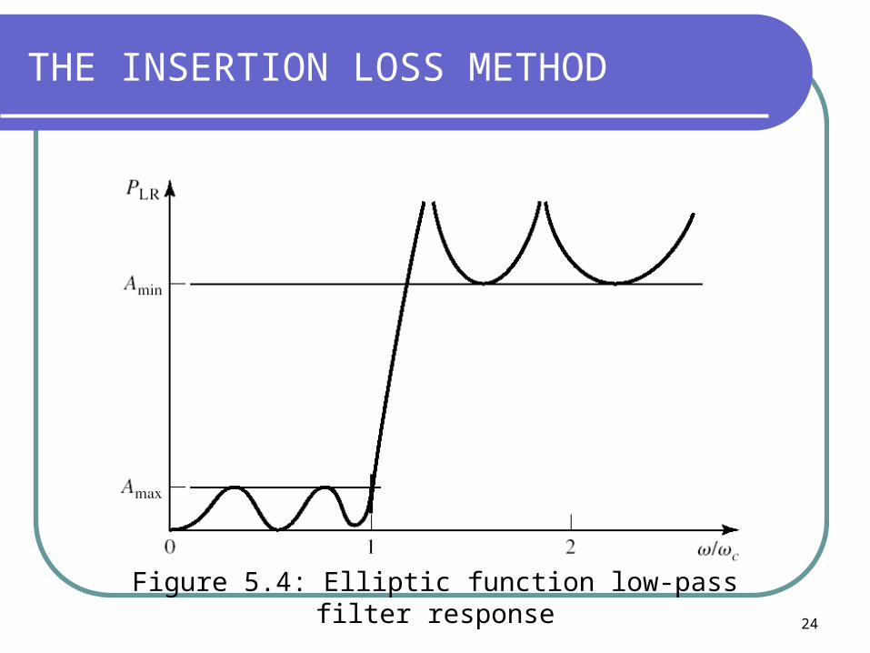
Elliptic function:- have equal ripple responses in the passband and stopband.- maximum attenuation in the passband.- minimum attenuation in the stopband.
Linear phase:- linear phase characteristic in the passband- to avoid signal distortion- maximally flat function for the group delay.
24
THE INSERTION LOSS METHOD
Figure 5.4: Elliptic function low-pass filter response

25
THE INSERTION LOSS METHOD
Filter Specification
Low-pass Prototype
Design
Scaling & Conversion
Filter Implementation
Optimization & Tuning
Normally done using simulators
Figure 5.5: The process of the filter design by the insertion loss method.

26
THE INSERTION LOSS METHOD
Figure 5.6: Low pass filter prototype, N = 2
Low Pass Filter Prototype

27
THE INSERTION LOSS METHOD
Figure 5.7: Ladder circuit for low pass filter prototypes and their element definitions. (a) begin with shunt element. (b) begin with
series element.
Low Pass Filter Prototype – Ladder Circuit

28
THE INSERTION LOSS METHOD
g0 = generator resistance, generator conductance.
gk = inductance for series inductors, capacitance for shunt capacitors.(k=1 to N)
gN+1 = load resistance if gN is a shunt capacitor, load conductance if gN is a series inductor.
As a matter of practical design procedure, it will be necessary to determine the size, or order of the filter. This is usually dictated by a specification on the insertion loss at some frequency in the stopband of the filter.

29
THE INSERTION LOSS METHOD
Figure 4.8: Attenuation versus normalized frequency for maximally flat filter prototypes.
Low Pass Filter Prototype – Maximally Flat

30
THE INSERTION LOSS METHOD
Figure 4.9: Element values for maximally flat LPF prototypes

31
THE INSERTION LOSS METHOD
221 NLR TkP
For an equal ripple low pass filter with a cutoff frequency ωc = 1, The power loss ratio is:
1
0NT
[5.12]
Where 1 + k2 is the ripple level in the passband. Since the Chebyshev polynomials have the property that
[5.12] shows that the filter will have a unity power loss ratio at ω = 0 for N odd, but the power loss ratio of 1 + k2 at ω = 0 for N even.
Low Pass Filter Prototype – Equal Ripple
32
THE INSERTION LOSS METHOD
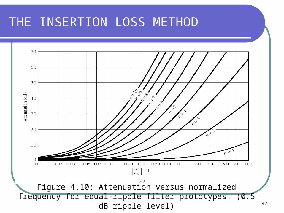
Figure 4.10: Attenuation versus normalized frequency for equal-ripple filter prototypes. (0.5 dB ripple level)

33
THE INSERTION LOSS METHOD
Figure 4.11: Element values for equal ripple LPF prototypes (0.5 dB ripple level)

34
THE INSERTION LOSS METHOD
Figure 4.12: Attenuation versus normalized frequency for equal-ripple filter prototypes (3.0 dB ripple level)

35
THE INSERTION LOSS METHOD
Figure 4.13: Element values for equal ripple LPF prototypes (3.0 dB ripple level).

36
FILTER TRANSFORMATIONS
LL
s
RRR
RR
R
CC
LRL
0'
0'
0
'
0'
[8.13a]
[8.13b]
[8.13c]
[8.13d]
Low Pass Filter Prototype – Impedance Scaling

37
FILTER TRANSFORMATIONS
'
'
kkc
k
kkc
k
CjCjjB
LjLjjX
The new element values of the prototype filter:
c
Frequency scaling for the low pass filter:
[8.14]
[8.15a]
[8.15b]

38
FILTER TRANSFORMATIONS
The new element values are given by:
c
kkk
c
kkk
R
CCC
LRLL
0
'
0'
[8.16a]
[8.16b]
39
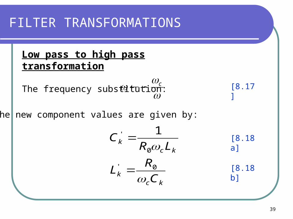
FILTER TRANSFORMATIONS
c
Low pass to high pass transformation
The frequency substitution:
kck
kck
C
RL
LRC
0'
0
' 1
The new component values are given by:
[8.17]
[8.18a]
[8.18b]
40
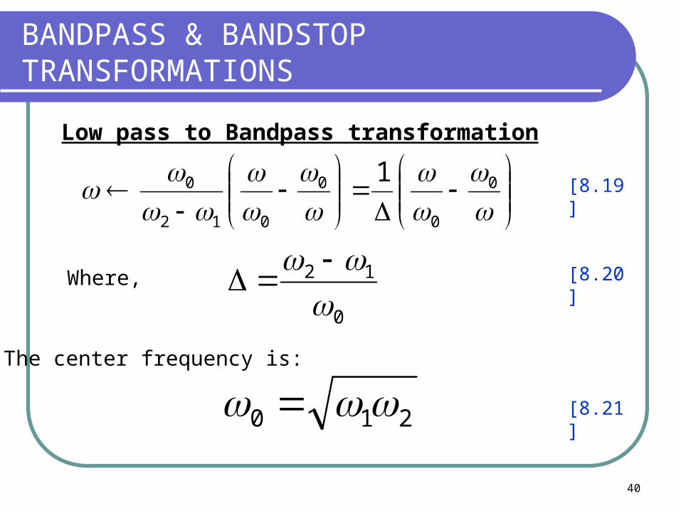
BANDPASS & BANDSTOP TRANSFORMATIONS
0
0
0
012
0 1
0
12
210
Where,
The center frequency is:
[8.19]
[8.20]
[8.21]
Low pass to Bandpass transformation

41
BANDPASS & BANDSTOP TRANSFORMATIONS
kk
kk
LC
LL
0
'
0
'
The series inductor, Lk, is transformed to a series LC circuit with element values:
The shunt capacitor, Ck, is transformed to a shunt LC circuit with element values:
0
'
0
'
kk
kk
CC
CL
[8.22a]
[8.22b]
[8.23a]
[8.23b]
42
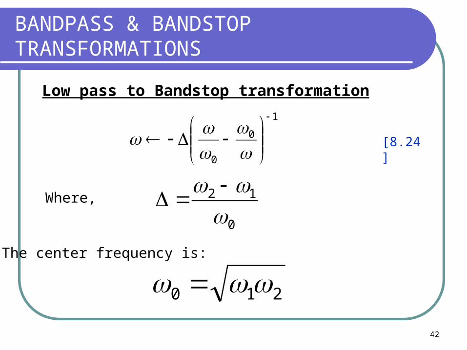
BANDPASS & BANDSTOP TRANSFORMATIONS
1
0
0
0
12
210
Where,
The center frequency is:
[8.24]
Low pass to Bandstop transformation

43
BANDPASS & BANDSTOP TRANSFORMATIONS
kk
kk
LC
LL
0
'
0
'
1
The series inductor, Lk, is transformed to a parallel LC circuit with element values:
The shunt capacitor, Ck, is transformed to a series LC circuit with element values:
0
'
0
' 1
kk
kk
CC
CL
[8.25a]
[8.25b]
[8.26a]
[8.26b]

44
BANDPASS & BANDSTOP TRANSFORMATIONS

45
EXAMPLE 5.1
Design a maximally flat low pass filter with a cutoff freq of 2 GHz, impedance of 50 Ω, and at least 15 dB insertion loss at 3 GHz. Compute and compare with an equal-ripple (3.0 dB ripple) having the same order.

46
EXAMPLE 5.1 (Cont)
Solution: First find the order of the maximally flat filter to satisfy the insertion loss specification at 3 GHz.
618.0
618.1
0.2
618.1
618.0
5
4
3
2
1
g
g
g
g
g
We can find the normalized freq by using: 5.012
31
c

47
EXAMPLE 5.1 (Cont)
The ladder diagram of the LPF prototype to be used is as follow:
LL
s
RRR
RR
R
CC
LRL
0'
0'
0
'
0'
C3 C5
L2 L4
C1
cR
gC
0
11
c
gRL
20
2
cR
gC
0
33
c
gRL
40
4
cR
gC
0
55

48
EXAMPLE 5.1 (Cont)
984.0102250
618.09
0
11
cR
gC
438.61022
618.1509
202
c
gRL
183.3102250
00.29
0
33
cR
gC
438.61022
618.1509
404
c
gRL
984.0102250
618.09
0
55
cR
gC
pF
nH
pF
nH
pF
LPF prototype for maximally flat filter

49
EXAMPLE 5.1 (Cont)
541.5102250
4817.39
0
11
cR
gC
031.31022
7618.0509
202
c
gRL
223.7102250
5381.49
0
33
cR
gC
031.31022
7618.0509
404
c
gRL
541.5102250
4817.39
0
55
cR
gC
pF
nH
pF
nH
pF
4817.3
7618.0
5381.4
7618.0
4817.3
5
4
3
2
1
g
g
g
g
g
LPF prototype for equal ripple filter:

50
THE INSERTION LOSS METHOD
Filter Specification
Low-pass Prototype
Design
Scaling & Conversion
Filter Implementation
Optimization & Tuning
Normally done using simulators

51
SUMMARY OF STEPS IN FILTER DESIGN
A. Filter Specification
1. Max Flat/Equal Ripple,
2. If equal ripple, how much pass band ripple allowed? If max
flat filter is to be designed, cont to next step
3. Low Pass/High Pass/Band Pass/Band Stop
4. Desired freq of operation
5. Pass band & stop band range
6. Max allowed attenuation (for Equal Ripple)

52
SUMMARY OF STEPS IN FILTER DESIGN (cont)
B. Low Pass Prototype Design
1. Min Insertion Loss level, No of Filter
Order/Elements by using IL values
2. Determine whether shunt cap model or series
inductance model to use
3. Draw the low-pass prototype ladder diagram
4. Determine elements’ values from Prototype Table

53
SUMMARY OF STEPS IN FILTER DESIGN (cont)
C. Scaling and Conversion
1. Determine whether if any modification to the
prototype table is required (for high pass, band
pass and band stop)
2. Scale elements to obtain the real element values
54
SUMMARY OF STEPS IN FILTER DESIGN (cont)
D. Filter Implementation
1. Put in the elements and values calculated from
the previous step
2. Implement the lumped element filter onto a
simulator to get the attenuation vs frequency
response

55
EXAMPLE 5.2
Design a band pass filter having a 0.5 dB equal-ripple response, with N = 3. The center frequency is 1 GHz, the bandwidth is 10%, and the impedance is 50 Ω.
56
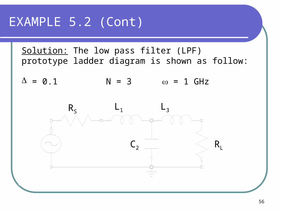
EXAMPLE 5.2 (Cont)
Solution: The low pass filter (LPF) prototype ladder diagram is shown as follow:
= 0.1 N = 3 = 1 GHz
CAPID=C1C=5.15 pF
INDID=L1L=15.91 nH
INDID=L2L=4.918 nH
ACCSID=I1Mag=1 mAAng=0 DegOffset=0 mADCVal=0 mA
RESID=R1R=1 Ohm
RESID=R2R=1 Ohm
RSL1 L3
C2 RL

57
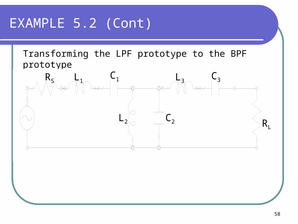
EXAMPLE 5.2 (Cont)
From the equal ripple filter table (with 0.5 dB ripple), the filter elements are as follow;
LRg
Lg
Cg
Lg
000.1
5963.1
0967.1
5963.1
4
33
2
1
2
1
58
EXAMPLE 5.2 (Cont)
Transforming the LPF prototype to the BPF prototype
INDID=L2L=1 nH
CAPID=C1C=1 pF
CAPID=C2C=1 pF
ACCSNID=I1Mag=10 mAAng=0 DegF=1 GHzTone=2Offset=0 mADCVal=0 mA
RESID=R1R=1 Ohm RES
ID=R2R=1 Ohm
INDID=L1L=1 nH
INDID=L3L=1 nH
CAPID=C3C=1 pF
RS
RL
C1
C2
C3L1
L2
L3

59
EXAMPLE 5.2 (Cont)
pFLZ
C 199.05963.1102250
1.09
1001
nHZL
L 0.1271.01012
505963.19
0
1
1
0
pFZ
CC 91.34
50)1.0(1012
0967.19
00
22
nHC
ZL 726.0
0967.11012
501.09
20
02
60
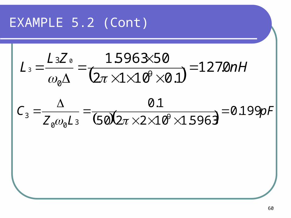
EXAMPLE 5.2 (Cont)
pFLZ
C 199.05963.1102250
1.09
3003
nHZL
L 0.1271.01012
505963.19
0
3 0
3

61
EXAMPLE 5.3
Design a five-section high pass lumped element filter with 3 dB equal-ripple response, a cutoff frequency of 1 GHz, and an impedance of 50 Ω. What is the resulting attenuation at 0.6 GHz?
62
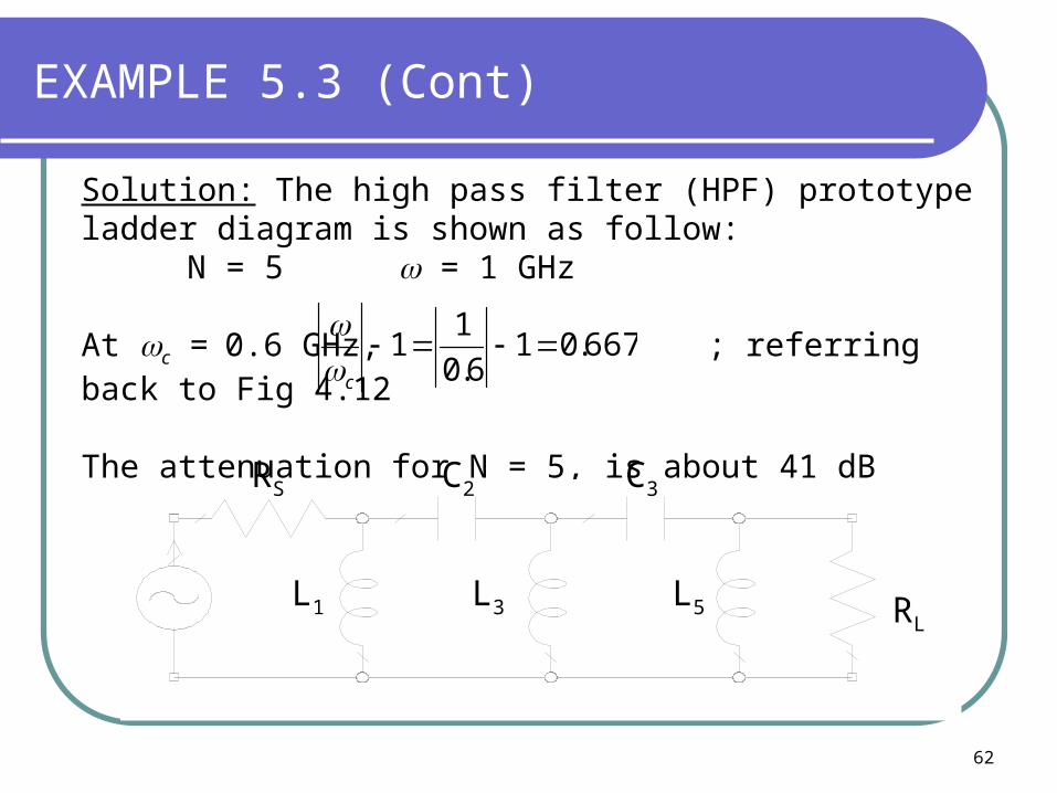
EXAMPLE 5.3 (Cont)
Solution: The high pass filter (HPF) prototype ladder diagram is shown as follow:
N = 5 = 1 GHz
At c = 0.6 GHz, ; referring back to Fig 4.12
The attenuation for N = 5, is about 41 dB
INDID=L1L=1 nH
INDID=L2L=1 nH
INDID=L3L=1 nH
CAPID=C1C=1 pF
CAPID=C2C=1 pF
ACCSNID=I1Mag=10 mAAng=0 DegF=1 GHzTone=2Offset=0 mADCVal=0 mA
RESID=R1R=1 Ohm
RESID=R2R=1 Ohm
RS
RLL1 L3 L5
C2 C3
667.016.0
11
c
63
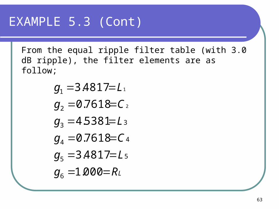
EXAMPLE 5.3 (Cont)
From the equal ripple filter table (with 3.0 dB ripple), the filter elements are as follow;
LRg
Lg
Cg
Lg
Cg
Lg
000.1
4817.3
7618.0
5381.4
7618.0
4817.3
6
55
44
33
2
1
2
1

64
EXAMPLE 5.3 (Cont)
pFCZ
Cc
18.47618.0101250
11'
920
2
nHL
ZL
c
28.24817.31012
50'
91
1
0
nHL
ZL
c
754.15381.41012
50'
93
03
Impedance and frequency scaling:

65
EXAMPLE 5.3 (Cont)
pFCZ
Cc
18.47618.0101250
11'
940
4
nHL
ZL
c
754.15381.41012
50'
95
05

66
EXAMPLE 5.4
Design a 4th order Butterworth Low-Pass Filter. Rs = RL= 50Ohm, fc = 1.5GHz.
L1=0.7654H L2=1.8478H
C1=1.8478F C2=0.7654FRL= 1g0= 1
L1=4.061nH L2=9.803nH
C1=3.921pF C2=1.624pFRL= 50g0=1/50
noRZR
c
no
LZL
co
n
Z
CC
50Z
rad/s 104248.95.12
o
9
GHzc
Step 1&2: LPP
Step 3: Frequency scalingand impedance denormalization
67
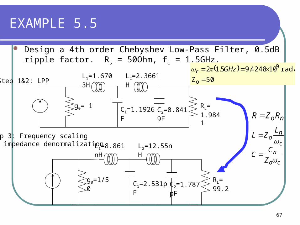
EXAMPLE 5.5
Design a 4th order Chebyshev Low-Pass Filter, 0.5dB ripple factor. Rs = 50Ohm, fc = 1.5GHz.
L1=1.6703H L2=2.3661H
C1=1.1926F C2=0.8419FRL= 1.9841
g0= 1
L1=8.861nH L2=12.55nH
C1=2.531pF C2=1.787pFRL= 99.2
g0=1/50
noRZR
c
no
LZL
co
n
Z
CC
50Z
rad/s 104248.95.12
o
9
GHzc
Step 1&2: LPP
Step 3: Frequency scalingand impedance denormalization

68
EXAMPLE 5.6
Design a bandpass filter with Butterworth (maximally flat) response.
N = 3. Center frequency fo = 1.5GHz.
3dB Bandwidth = 200MHz or f1=1.4GHz, f2=1.6GHz.

69
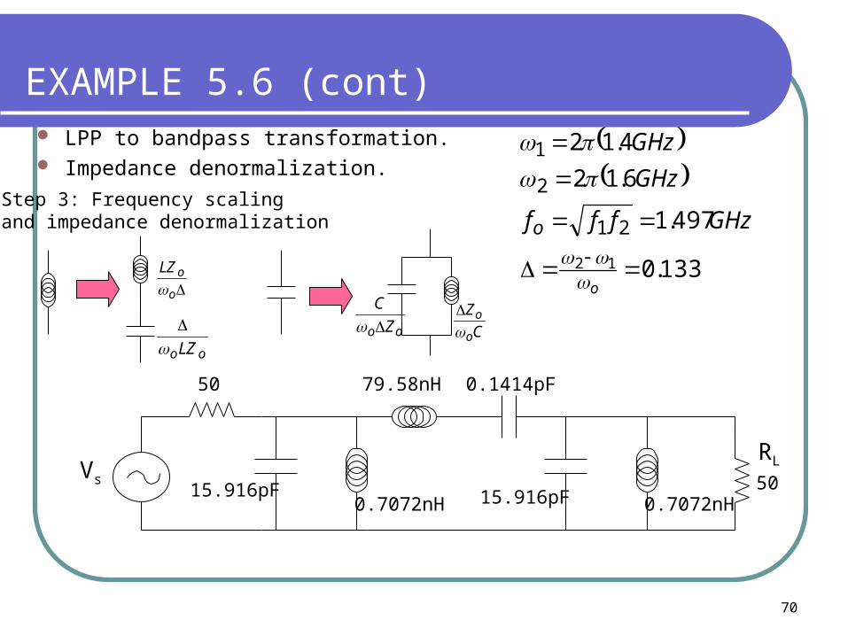
EXAMPLE 5.6 (cont)
From table, design the Low-Pass prototype (LPP) for 3rd order Butterworth response, c=1.
Zo=1
g1 1.000F
g3 1.000F
g2 2.000H
g4
12<0o
Hz 1592.0
12
21
c
cc
f
f
Step 1&2: LPP
70
EXAMPLE 5.6 (cont) LPP to bandpass transformation. Impedance denormalization.
133.0
497.1
6.12
4.12
12
21
2
1
o
GHzfff
GHz
GHz
o
50
Vs15.916pF
0.1414pF79.58nH
0.7072nH 0.7072nH15.916pF50
RL
o
oLZ
ooLZ oo Z
C
C
Z
o
o
Step 3: Frequency scalingand impedance denormalization


