1. Expected utility, risk aversion and stochastic dominance

1.1 Expected utility

1.1.1 Description of risky alternatives1.1.2 Preferences over lotteries1.1.3 The expected utility theorem

1.2 Monetary lotteries and risk aversion

1.2.1 Monetary lotteries and the expected utility framework1.2.2 Risk aversion1.2.3 Measures of risk aversion1.2.4 Risk aversion and portfolio selection

1.3 Stochastic dominance

1.3.1 First degree stochastic dominance1.3.2 Second degree stochastic dominance1.3.3 Second degree stochastic monotonic dominance

1

The objective of this part is to examine the choice of under uncertainty. We divide

this chapter in 3 sections.

The first part begins by developing a formal apparatus for modeling risk. We then

apply this framework to the study of preferences over risky alternatives. Finally,

we examine conditions of the preferences that guarantee the existence of a utility

function that represents these preferences.

In the second part, we focus on the particular case in which the outcomes are

monetary payoffs. Obviously, this case is very interesting in the area of finance. In

this part we present the concept of risk aversion and its measures.

In the last part, we are interested in the comparison of two risky assets in the case

in which we have a limited knowledge of individuals’ preferences. This

comparison leads us to the three concepts of stochastic dominance.

2

1.1 Expected utility

1.1.1 Description of risky alternatives

Let us suppose that an agent faces a choice among a number of risky alternatives.

Each risky alternative may result in one of a number of possible outcomes, but

which outcome will occur is uncertain at the time that he must make his choice.

Notation:

X = The set of all possible outcomes.

Examples:

X= A set of consumption bundles.

X= A set of monetary payoffs.

To simplify, in this part we make the following assumptions:

1. The number of possible outcomes of X is finite.

2. The probabilities of the different outcomes in a risky alternative are

objectively known.

The concept used to represent a risky alternative is the lottery.

Definition:

A simple lottery L is a list ( )nn ppxxxL ,...,;,...,, 121= , where

i) niXxi ,,1 , =∈

ii) 0≥ip and 11

=∑=

n

iip , where ip is interpreted as the probability of

outcome ix occurring.

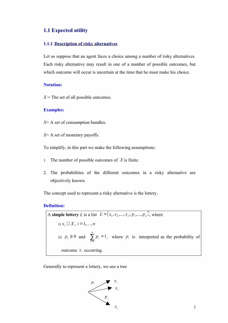
Generally to represent a lottery, we use a tree

3

x1

x2

xn

p1

pn

Notice that in a simple lottery the outcomes are certain. A more general concept, a

compound lottery, allows the outcomes of a lottery themselves to be simple

lotteries.

Definition:

Given K simple lotteries kL , Kk ,...1= , and probabilities 0≥kα with 11

=∑=

K

kkα ,

the compound lottery ( )KKLL αα ,...;,..., 11 is the risky alternative that yields the

simple lottery kL with probability kα , Kk ,...1= .

For any compound lottery, we can calculate its reduced lottery that is a simple

lottery that generates the same distribution over the final outcomes.

Exercise: (Illustration of the derivation of a reduced lottery)

4

1.1. 2 Preferences over lotteries

Having introduced a way to model risky alternatives, we now study the

preferences over them corresponding to a fixed agent. In this part we assume that

for any risky alternative, only the reduced lottery over final outcomes is of

relevance to the agent. This means that given two different compound lotteries

with the same reduced lottery, the decision maker is indifferent between them.

Let denote the set of all simple lotteries over the set of outcomes X. According

to the previous assumption we assume that the agent’s preferences (≳) are defined

on .

We make the following assumptions

A.1 The decision maker has a preference relation ≳ on . This means that ≳

satisfy the following properties:

1. ≳ is reflexive ( ,∈∀L L≳L)

2. ≳ is complete ( ,, 21 ∈∀ LL we either have L1≳L2 or L2≳L1 )

3. ≳ is transitive ( ,,, 321 ∈∀ LLL such that L1≳L2 and L2≳L3 , then L1≳L3)

A.2 The Archimedian Axiom:

,,, 321 ∈∀ LLL such that L1≻L2 ≻L3 , then there exists ( )1,0, ∈βα such that

31 )1( LL αα −+ ≻ L2 ≻ 31 )1( LL ββ −+

Economic intuition:

As L1≻L2, no matter how bad L3 is, we can combine L1 and L3 with α large

enough (near to one) such that 31 )1( LL αα −+ ≻ L2.

As L2≻L3, no matter how good L1 is, we can combine L1 and L3 with β small

enough (near to zero) such that L2 ≻ 31 )1( LL ββ −+ .

A.3 The Independence Axiom:

5

,,, 321 ∈∀ LLL and ]1,0(∈α

L1≻L2 if and only if 31 )1( LL αα −+ ≻ 32 )1( LL αα −+

Economic intuition:

If we combine two lotteries, L1 and L2, with a third lottery in the same way, the

preference ordering of the resulting lotteries does not depend on the third lottery.

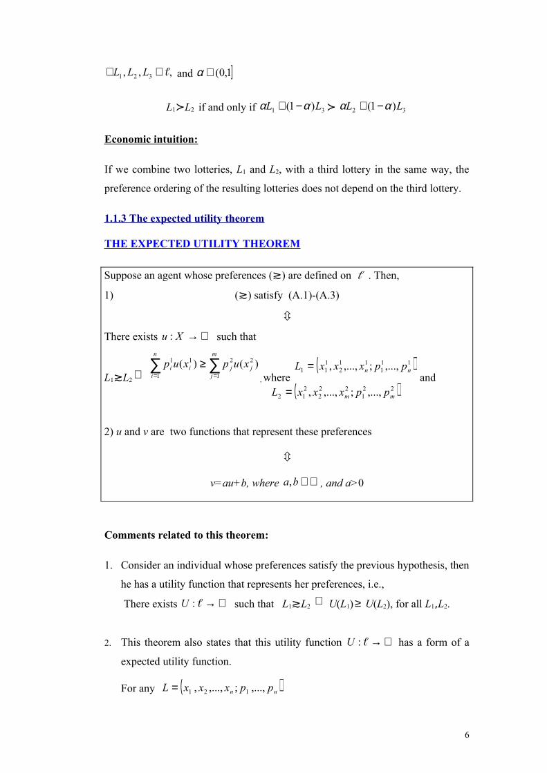
1.1.3 The expected utility theorem

THE EXPECTED UTILITY THEOREM

Suppose an agent whose preferences (≳) are defined on . Then,

1) (≳) satisfy (A.1)-(A.3)

There exists ℜ→Xu : such that

L1≳L2⇔

∑∑==

≥m

jjj

n

iii xupxup

1

22

1

11 )()(, where

( )111

112

111 ,...,;,...,, nn ppxxxL =

and

( )221

222

212 ,...,;,...,, mm ppxxxL =

2) u and v are two functions that represent these preferences

v=au+b, where ℜ∈ba, , and a>0

Comments related to this theorem:

1. Consider an individual whose preferences satisfy the previous hypothesis, then

he has a utility function that represents her preferences, i.e.,

There exists ℜ→:U such that L1≳L2 ⇔ U(L1)≥ U(L2), for all L1,L2.

2. This theorem also states that this utility function ℜ→:U has a form of a

expected utility function.

For any ( )nn ppxxxL ,...,;,...,, 121=

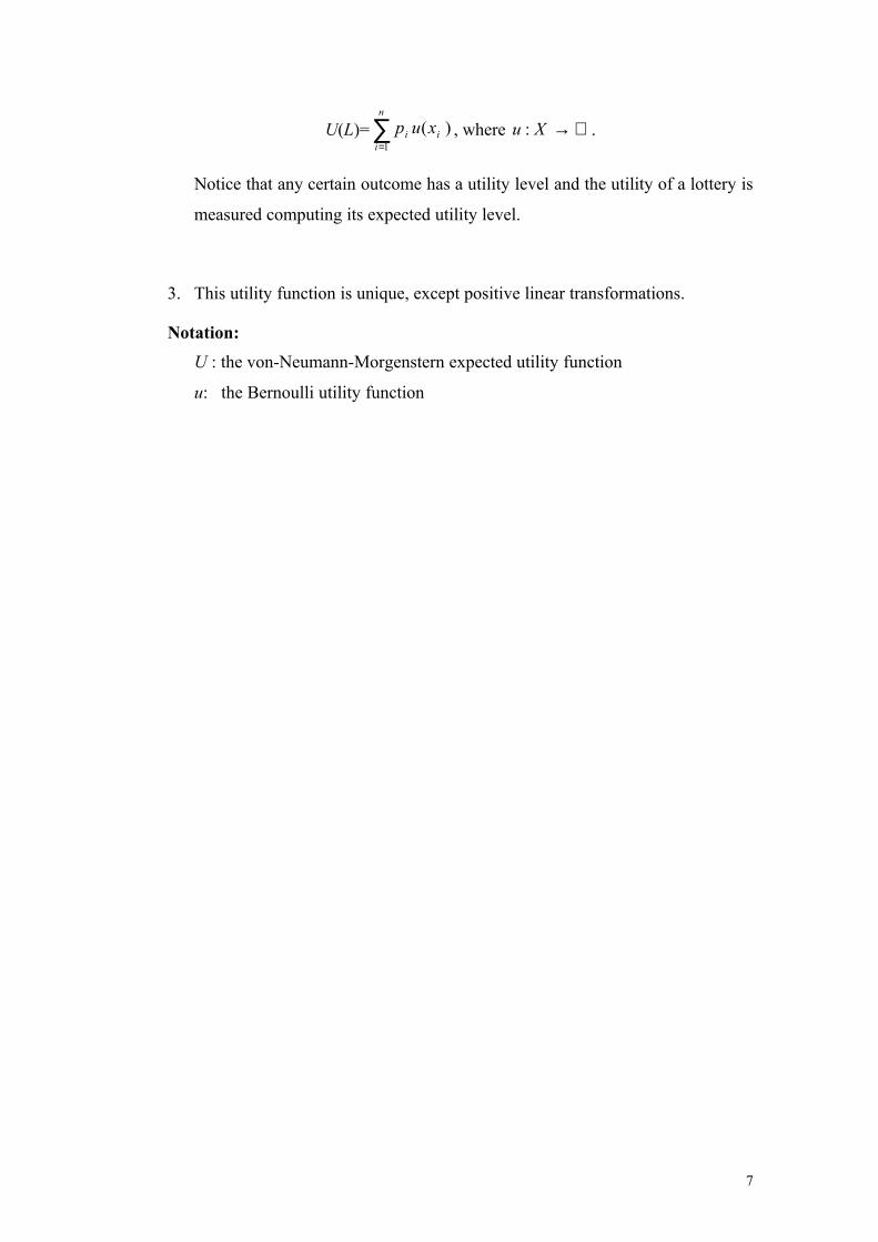
6

U(L)=∑=

n

iii xup

1

)( , where ℜ→Xu : .

Notice that any certain outcome has a utility level and the utility of a lottery is

measured computing its expected utility level.

3. This utility function is unique, except positive linear transformations.

Notation:

U : the von-Neumann-Morgenstern expected utility function

u: the Bernoulli utility function

7

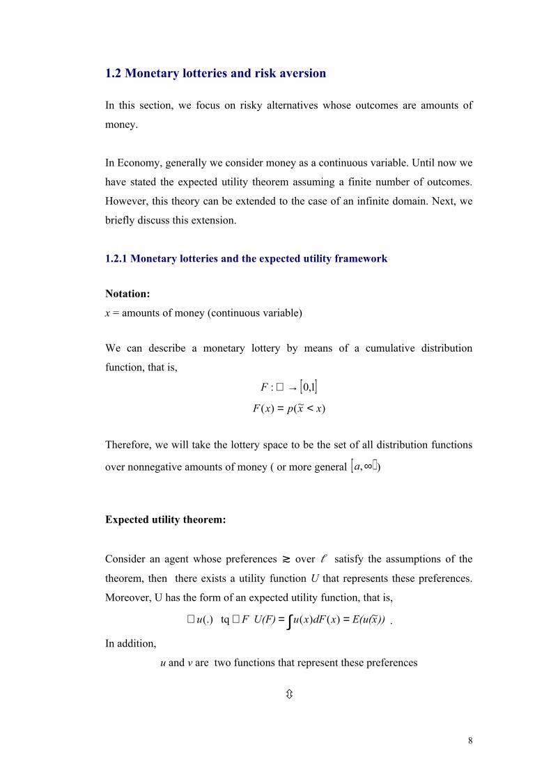
1.2 Monetary lotteries and risk aversion

In this section, we focus on risky alternatives whose outcomes are amounts of

money.

In Economy, generally we consider money as a continuous variable. Until now we

have stated the expected utility theorem assuming a finite number of outcomes.

However, this theory can be extended to the case of an infinite domain. Next, we

briefly discuss this extension.

1.2.1 Monetary lotteries and the expected utility framework

Notation:

x = amounts of money (continuous variable)

We can describe a monetary lottery by means of a cumulative distribution

function, that is,

[ ]1,0: →ℜF

)~()( xxpxF <=

Therefore, we will take the lottery space to be the set of all distribution functions

over nonnegative amounts of money ( or more general [ )∞,a )

Expected utility theorem:

Consider an agent whose preferences ≳ over satisfy the assumptions of the

theorem, then there exists a utility function U that represents these preferences.

Moreover, U has the form of an expected utility function, that is,

)) xE(u(xdFxuU(F)Fu ~)()( tq(.) ==∀∃ ∫ .

In addition,

u and v are two functions that represent these preferences

8

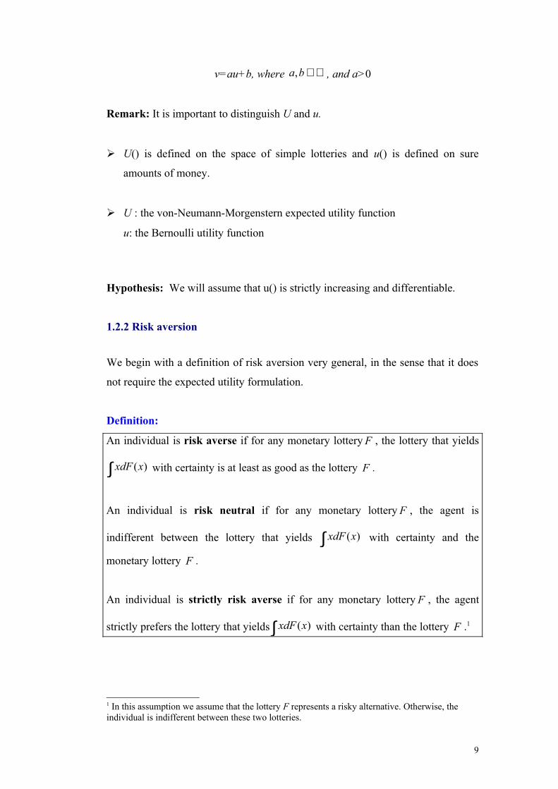
v=au+b, where ℜ∈ba, , and a>0

Remark: It is important to distinguish U and u.

U() is defined on the space of simple lotteries and u() is defined on sure

amounts of money.

U : the von-Neumann-Morgenstern expected utility function

u: the Bernoulli utility function

Hypothesis: We will assume that u() is strictly increasing and differentiable.

1.2.2 Risk aversion

We begin with a definition of risk aversion very general, in the sense that it does

not require the expected utility formulation.

Definition:

An individual is risk averse if for any monetary lottery F , the lottery that yields

∫ )(xxdF with certainty is at least as good as the lottery F .

An individual is risk neutral if for any monetary lottery F , the agent is

indifferent between the lottery that yields ∫ )(xxdF with certainty and the

monetary lottery F .

An individual is strictly risk averse if for any monetary lottery F , the agent

strictly prefers the lottery that yields ∫ )(xxdF with certainty than the lottery F .1

1 In this assumption we assume that the lottery F represents a risky alternative. Otherwise, the individual is indifferent between these two lotteries.

9

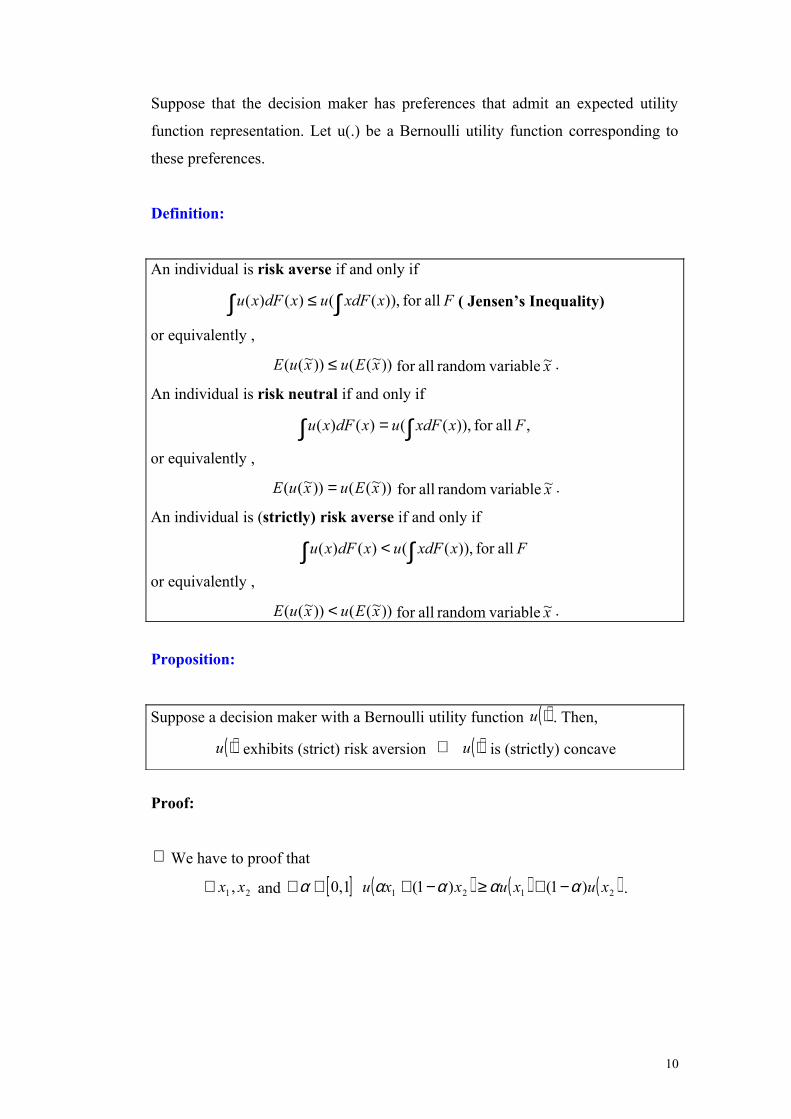
Suppose that the decision maker has preferences that admit an expected utility

function representation. Let u(.) be a Bernoulli utility function corresponding to

these preferences.

Definition:

An individual is risk averse if and only if

FxxdFuxdFxu allfor ),)(()()( ∫∫ ≤ ( Jensen’s Inequality)

or equivalently ,

))~(())~(( xEuxuE ≤ x~ variablerandom allfor .

An individual is risk neutral if and only if

, allfor ),)(()()( FxxdFuxdFxu ∫∫ =

or equivalently ,

))~(())~(( xEuxuE = x~ variablerandom allfor .

An individual is (strictly) risk averse if and only if

FxxdFuxdFxu allfor ),)(()()( ∫∫ <

or equivalently ,

))~(())~(( xEuxuE < x~ variablerandom allfor .

Proposition:

Suppose a decision maker with a Bernoulli utility function ( )⋅u . Then,

( )⋅u exhibits (strict) risk aversion ⇔ ( )⋅u is (strictly) concave

Proof:

⇒We have to proof that

21 , xx∀ and [ ]0,1 ∈∀α ( ) ( ) ( )2121 )1()1( xuxuxxu αααα −+≥−+ .

10

Consider the following monetary lottery:

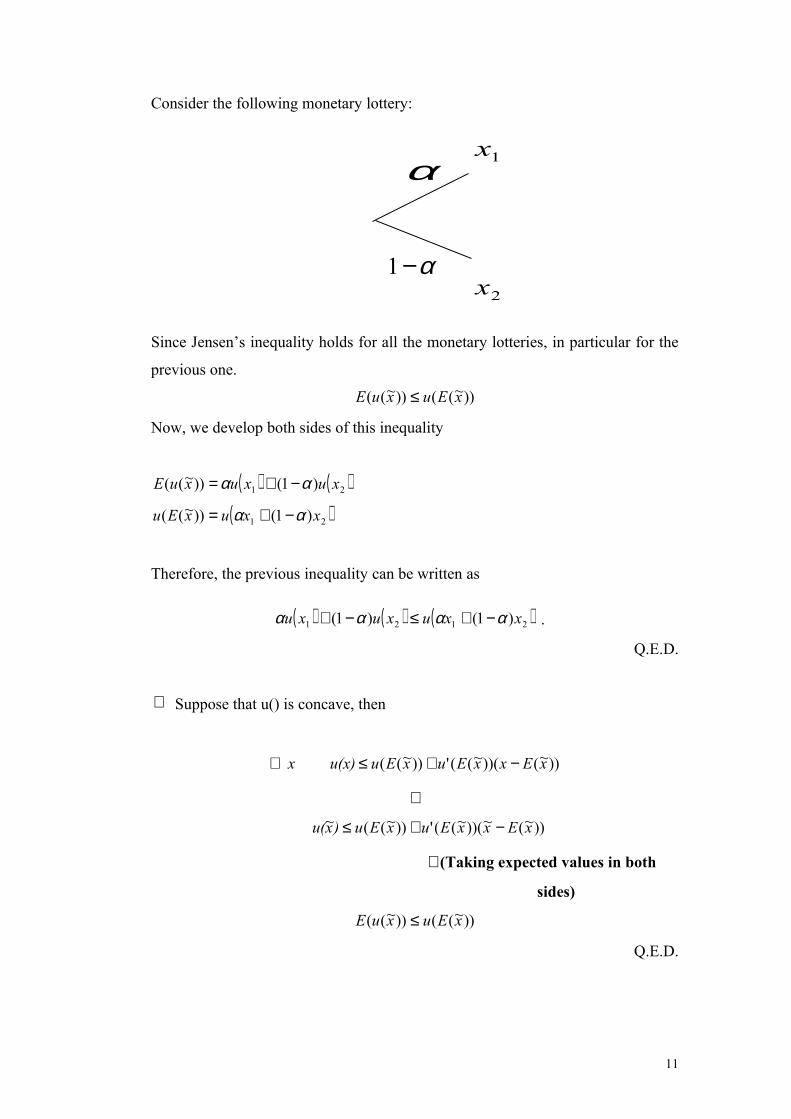
Since Jensen’s inequality holds for all the monetary lotteries, in particular for the

previous one.

))~(())~(( xEuxuE ≤

Now, we develop both sides of this inequality

( ) ( )21 )1())~(( xuxuxuE αα −+=

( )21 )1())~(( xxuxEu αα −+=

Therefore, the previous inequality can be written as

( ) ( ) ( )2121 )1()1( xxuxuxu αααα −+≤−+ .

Q.E.D.

⇐ Suppose that u() is concave, then

))~())(~(('))~(( xExxEuxEuu(x)x −+≤∀

⇓

))~(~))(~(('))~((~ xExxEuxEu)xu( −+≤

⇓ (Taking expected values in both

sides)

))~(())~(( xEuxuE ≤

Q.E.D.

11

1x

2x

α

α−1

Next we introduce two concepts related to risk aversion.

Consider a risk averse agent, with a Bernoulli utility function u(.) and an initial

wealth 0W . Let z~ denote the outcome of a gamble. By risk aversion, we have that

the individual prefers )~(zE to z~ , that is

))~(())~(( 00 zEWuzWuE +≤+ .

This inequality tells us that to avoid the risk the individual is willing to pay. The

maximum amount of money that the individual is willing to pay is called the

Pratt’s risk premium or insurance risk premium.

Definition:

Given a decision maker with a Bernoulli utility function u() and a initial wealth

0W , the Pratt’s risk premium or insurance risk premium of z~ is a certain

amount, denoted by )~(zΠ , such that

))~()~(())~(( 00 zzEWuzWuE Π−+=+ .

The certain amount )~()~(0 zzEW Π−+ is called certainty equivalent of z~ , since

it is the amount of money for which the individual is indifferent between z~ and

this certain amount.

Example: Let zWx ~~0 += . Suppose that it takes two values 21 and xx equally

likely.

12

The following example illustrates the use of the risk aversion concept.

Example: Demand for a risky asset

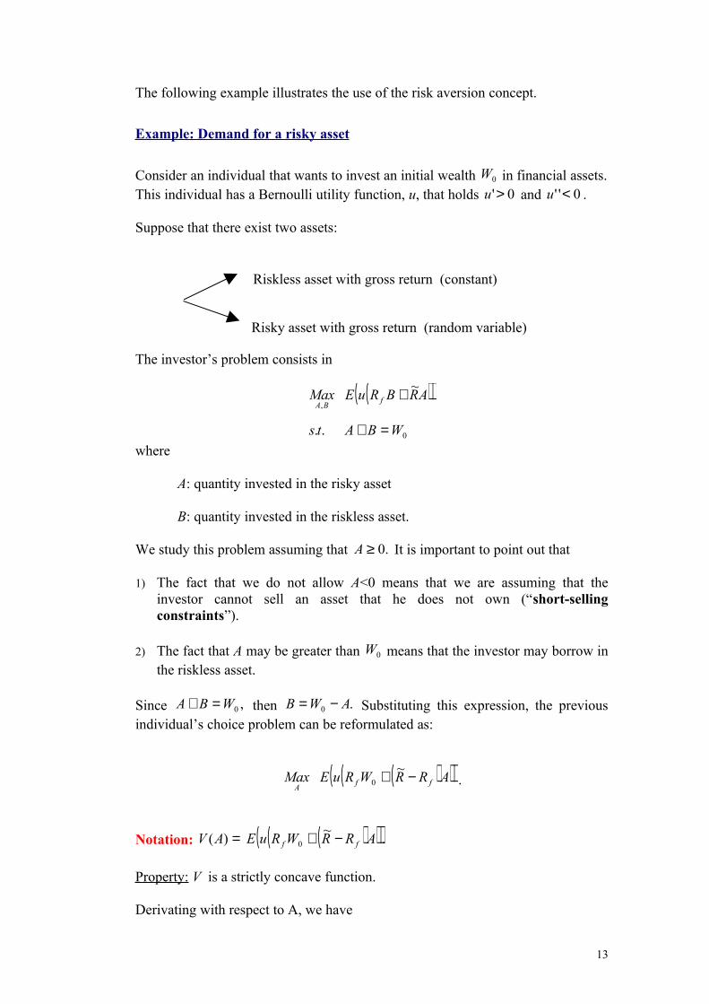
Consider an individual that wants to invest an initial wealth 0W in financial assets. This individual has a Bernoulli utility function, u, that holds 0'>u and 0'' <u .

Suppose that there exist two assets:

The investor’s problem consists in

( )( )0

,

..

~

WB Ats

ARBRuEMax fBA

=+

+

where

A: quantity invested in the risky asset

B: quantity invested in the riskless asset.

We study this problem assuming that .0≥A It is important to point out that

1) The fact that we do not allow A<0 means that we are assuming that the investor cannot sell an asset that he does not own (“short-selling constraints”).

2) The fact that A may be greater than 0W means that the investor may borrow in the riskless asset.

Since ,0WBA =+ then .0 AWB −= Substituting this expression, the previous individual’s choice problem can be reformulated as:

( )( )( )ARRWRuEMax ffA

−+ ~ 0 .

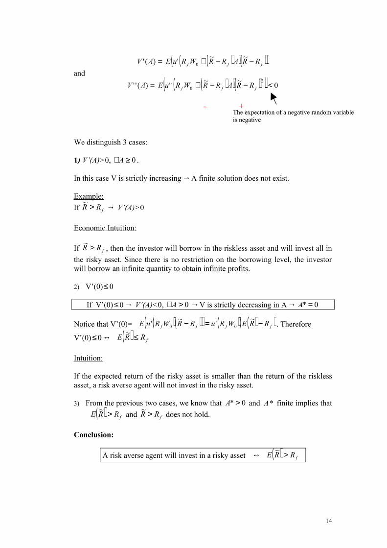
Notation: ( )( )( ).~ )( 0 ARRWRuEAV ff −+=

Property: V is a strictly concave function.

Derivating with respect to A, we have

13

Riskless asset with gross return (constant)

Risky asset with gross return (random variable)

( )( )( )( )fff RRARRWRuEAV −−+= ~~' )(' 0

and

( )( )( )( ) 0~~

'' )(''2

0 <−−+= fff RRARRWRuEAV

- +

We distinguish 3 cases:

1) V’(A)>0, 0≥∀A .

In this case V is strictly increasing →A finite solution does not exist.

Example:

If fRR >~ → V’(A)>0

Economic Intuition:

If fRR >~, then the investor will borrow in the riskless asset and will invest all in

the risky asset. Since there is no restriction on the borrowing level, the investor will borrow an infinite quantity to obtain infinite profits.

2) V’(0) ≤ 0

If V’(0) ≤ 0→ V’(A)<0, 0>∀A →V is strictly decreasing in A→ 0* =A

Notice that V’(0)= ( )( )( ) ( ) ( )( )ffff RREWRuRRWRuE −=− ~'

~' 00 . Therefore

V’(0) ≤ 0 ↔ ( ) fRRE ≤~

Intuition:

If the expected return of the risky asset is smaller than the return of the riskless asset, a risk averse agent will not invest in the risky asset.

3) From the previous two cases, we know that 0* >A and *A finite implies that

( ) fRRE >~ and fRR >~

does not hold.

Conclusion:

A risk averse agent will invest in a risky asset ↔ ( ) fRRE >~

14

The expectation of a negative random variable is negative

1.2.3 Measures of Risk Aversion

Now we try to measure the extent of risk aversion. We begin with the most used

measure of risk aversion which is the coefficient of absolute risk aversion (also

called the Arrow-Pratt’s coefficient)

The Coefficient of Absolute Risk Aversion

Motivation of the coefficient of absolute risk aversion:

Notice that risk aversion is equivalent to the concavity of u( ), that is, u’’≤ 0.

Therefore, it seems logical to start considering one possible measure: u’’.

However, this is not an adequate measure because is not invariant to positive

linear transformations. To make it invariant, the simplest modification is to

normalize with u’.

Definition:

Given a Bernoulli utility function u( ), the coefficient of absolute risk aversion

at x is defined as

)('

)('')(

xu

xuxRA −= .

Comments of this expression:

This measure is invariant to linear transformations.

The sign minus makes the expression be positive when u() is increasing and

concave.

Next, we use this measure in two comparative statics exercises.

1) Comparison of risk attitudes across individuals with different utility functions

2) Comparison of risk attitudes for one individual at different levels of wealth.

15

Comparison across individuals

Consider two individuals, individual 1 and individual 2, with two Bernoulli utility

functions 1u and 2u , respectively, such that:

1) 0'1 >u and 0'2 >u ,

2) 0''1 <u and 0''2 <u .

Next, we want to prove that the coefficient of absolute risk aversion is an effective

measure, that is, if individual 1 is more risk averse than individual 2, then it holds

)()( 21 xRxR AA ≥ , x∀ , and vice versa, where

.2,1 ,)('

)('')( =−= i

xu

xuxR

i

iiA .

Notice that individual 1 is more risk averse than individual 2

∃ G(.), strictly increasing and concave such that ))(()( 21 xuGxu = (“u1 is

more concave than u2”).

Therefore, we want to show

Lemma 1:

∃ G(.), strictly increasing and concave such that ))(()( 21 xuGxu =

⇔ )()( 21 xRxR AA ≥ , x∀

⇒ Suppose that ))(()( 21 xuGxu = . Then ,

)('))((')(' 221 xuxuGxu = and

( ) )(''))((')('))(('')('' 222

221 xuxuGxuxuGxu += .

Therefore,

( ))('))(('

)(''))((')('))((''

)('

)('')(

22

222

22

1

11

xuxuG

xuxuGxuxuG

xu

xuxRA

+−=−= =

=( )

)()('

)(''

)('))(('

)(''))(('

)('))(('

)('))(('' 2

2

2

22

22

22

222 xR

xu

xu

xuxuG

xuxuG

xuxuG

xuxuGA=−≥−− (*)

16

⇐ Now we assume that )()( 21 xRxR AA ≥ , x∀ .

Notice that since 1u and 2u are strictly increasing, it is true that exits G(.) such

that ))(()( 21 xuGxu = . (Notice that 121

−= uuG and it is differentiable).

Therefore, )('))((')(' 221 xuxuGxu = , which implies that G’>0.

Moreover, using (*), we know that

)(1 xRA =( )

)()('))(('

)('))(('' 2

22

222 xR

xuxuG

xuxuGA+− .

Using the fact that )()( 21 xRxR AA ≥ , the previous equality tells us that

( )0

)('))(('

)('))((''

22

222 ≥−

xuxuG

xuxuG, which implies that 0))(('' 2 ≤xuG because u2 and G

are strictly increasing functions.

Note:

The relation more-risk averse-than relation is a partial ordering of Bernoulli utility

functions, since it is not complete. Typically, given two Bernoulli utility

functions )()( 21 xRxR AA ≥ at some x, but the contrary inequality holds for

other levels.

Lemma 2:

Consider two individuals with strictly increasing and strictly concave Bernoulli

utility functions 1u and 2u , and with identical initial wealth 0W . Then

)()( 21 xRxR AA ≥ x∀ ⇔ )~()~( 21 zz Π≥Π z~∀

Proof: By Lemma 1, it suffices to show

∃ G(.) strictly increasing and concave such that ))(()( 21 xuGxu =

⇔ )~()~( 21 zz Π≥Π z~∀

⇒ Using the definition of the Pratt’s risk premium for the individual 1, we have

=+≤+=+=Π−+ )))~((()))~((())~(())~()~(( 020201101 zWuEGzWuGEzWuEzzEWu

( ) ))~()~(())~()~(( 201202 zzEWuzzEWuG Π−+=Π−+

17

Therefore,

≤Π−+ ))~()~(( 101 zzEWu ))~()~(( 201 zzEWu Π−+ .

Using the fact that u1 is strictly increasing , this inequality implies that

≤Π−+ )~()~( 10 zzEW )~()~( 20 zzEW Π−+ ,

or equivalently, )~()~( 21 zz Π≥Π .

⇐ Notice that since 1u and 2u are strictly increasing, it is true that exits G(.)

such that ))(()( 21 xuGxu = (Notice that 121

−= uuG and it is differentiable).

Therefore, )('))((')(' 221 xuxuGxu = , which implies that G’>0.

To show the concavity of G, we will prove Jensen’s inequality, that is,

))~(())~(( xEGxGE ≤ , x~∀ .

Fix x~ . Then there exists z~ such that )~(~02 zWux += . Therefore,

( )( ) ( )( ) =+=+= zWuEzWuGExGE ~)~())~(( 0102 ≤Π−+ ))~()~(( 101 zzEWu

( ) ( )( )( ) ( )( )xEGzWuEGzzEWuGzzEWu ~~))~()~(())~()~(( 02202201 =+=Π−+=Π−+

Comparison across wealth levels

Typically, richer people are more willing to accept risk than poorer people.

Although this might be due to differences in utility functions across people, it is

more likely that this is due to differences in the wealth levels. Then, the way to

formalize this risk attitude is to assume that )(xRA is a decreasing function of x.

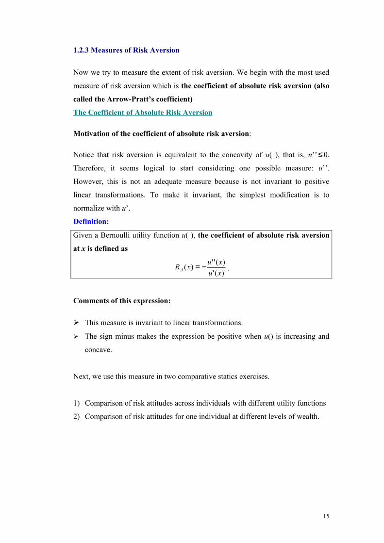
Lemma:

)(xRA is a decreasing function of x 0''' >⇒ u

18

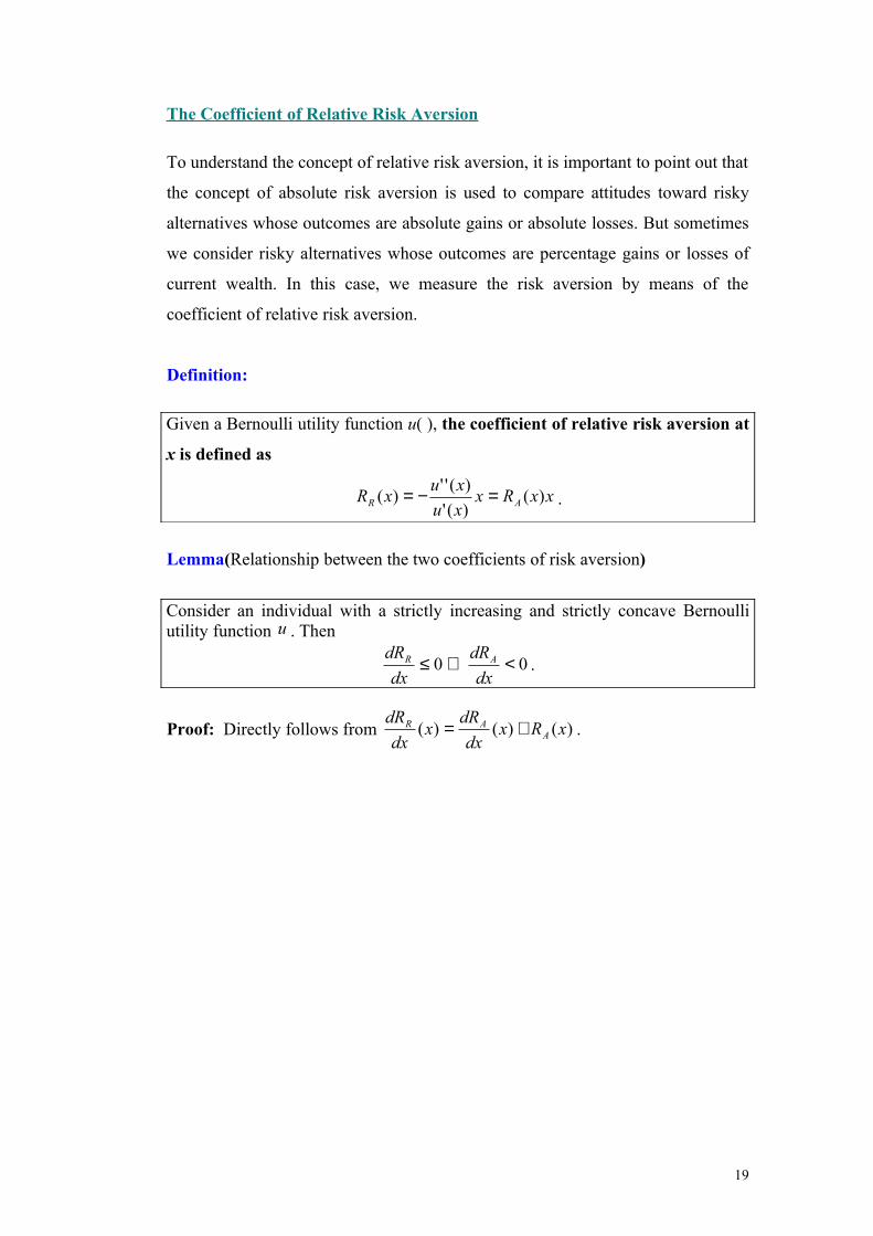
The Coefficient of Relative Risk Aversion

To understand the concept of relative risk aversion, it is important to point out that

the concept of absolute risk aversion is used to compare attitudes toward risky

alternatives whose outcomes are absolute gains or absolute losses. But sometimes

we consider risky alternatives whose outcomes are percentage gains or losses of

current wealth. In this case, we measure the risk aversion by means of the

coefficient of relative risk aversion.

Definition:

Given a Bernoulli utility function u( ), the coefficient of relative risk aversion at

x is defined as

xxRxxu

xuxR AR )(

)('

)('')( =−= .

Lemma(Relationship between the two coefficients of risk aversion)

Consider an individual with a strictly increasing and strictly concave Bernoulli utility function u . Then

00 <⇒≤dx

dR

dx

dR AR .

Proof: Directly follows from )()()( xRxdx

dRx

dx

dRA

AR += .

19

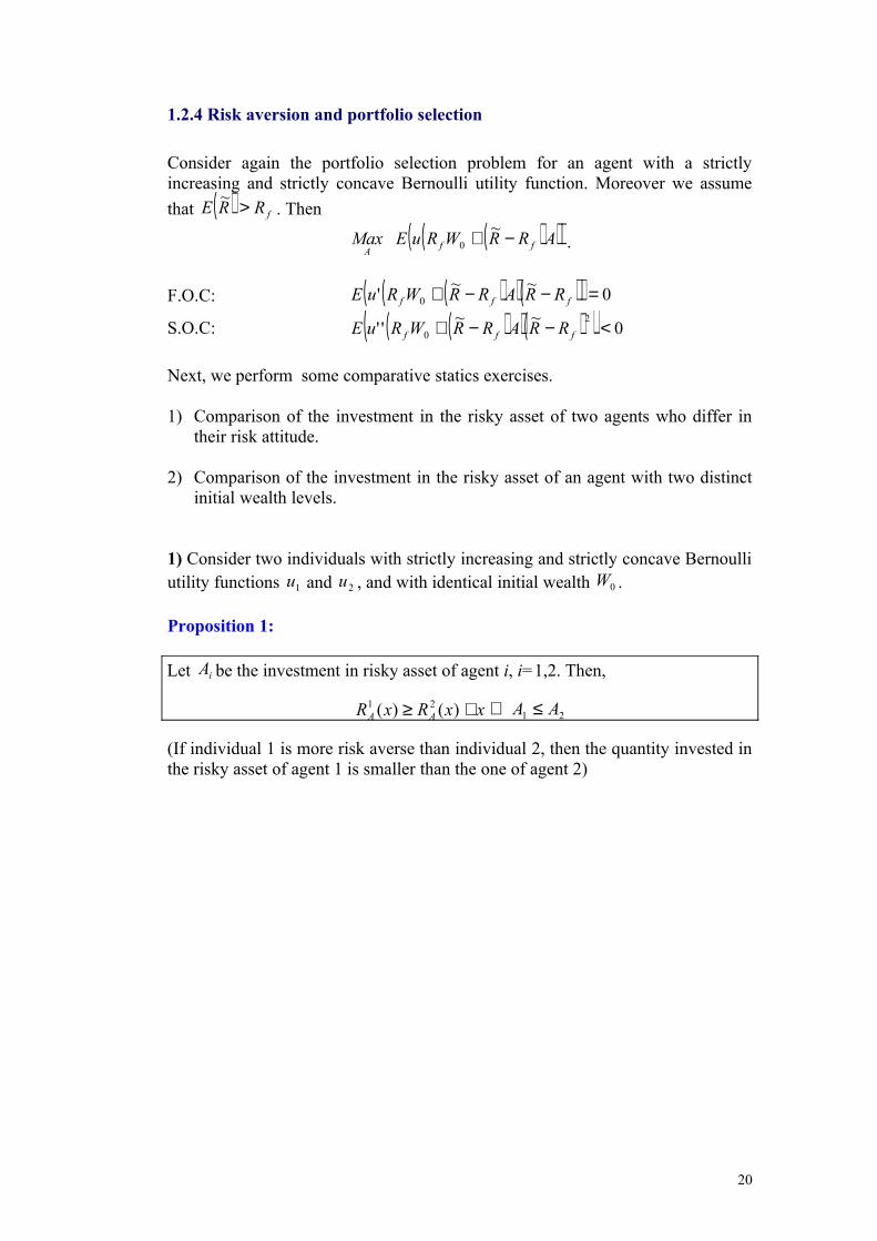
1.2.4 Risk aversion and portfolio selection

Consider again the portfolio selection problem for an agent with a strictly increasing and strictly concave Bernoulli utility function. Moreover we assume

that ( ) fRRE >~. Then

( )( )( )ARRWRuEMax ffA

−+ ~ 0 .

F.O.C: ( )( )( )( ) 0~~

' 0 =−−+ fff RRARRWRuE

S.O.C: ( )( )( )( ) 0~~

''2

0 <−−+ fff RRARRWRuE

Next, we perform some comparative statics exercises.

1) Comparison of the investment in the risky asset of two agents who differ in their risk attitude.

2) Comparison of the investment in the risky asset of an agent with two distinct initial wealth levels.

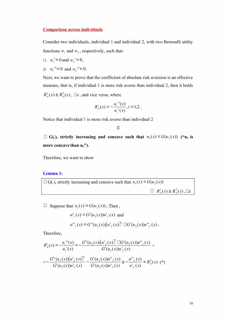
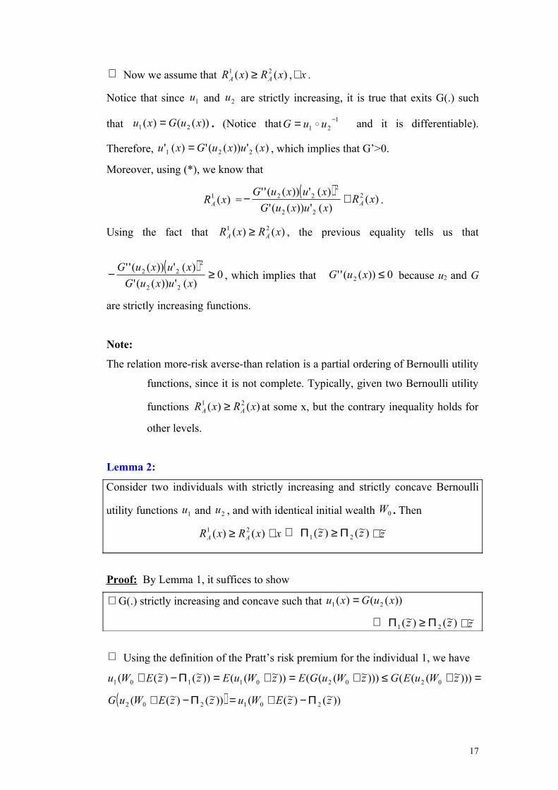
1) Consider two individuals with strictly increasing and strictly concave Bernoulli utility functions 1u and 2u , and with identical initial wealth 0W .

Proposition 1:

Let iA be the investment in risky asset of agent i, i=1,2. Then,

)()( 21 xRxR AA ≥ x∀ 21 AA ≤⇒

(If individual 1 is more risk averse than individual 2, then the quantity invested in the risky asset of agent 1 is smaller than the one of agent 2)

20

2) Now, we are interested in studying how vary the investment in the risky asset of an agent when her initial wealth varies.

Proposition 2:

0 0)(0

>⇒∀<dW

dAxx

dx

dRA

0 0)(0

=⇒∀=dW

dAxx

dx

dRA

0 0)(0

<⇒∀>dW

dAxx

dx

dRA

Suppose that an individual has a Bernoulli utility function that exhibits decreasing absolute risk aversion then if the agent becomes richer then he will invest more in the risky asset.

21

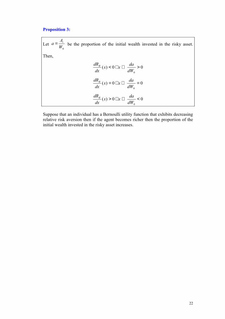
Proposition 3:

Let 0W

Aa i= be the proportion of the initial wealth invested in the risky asset.

Then,

0 0)(0

>⇒∀<dW

daxx

dx

dRR

0 0)(0

=⇒∀=dW

daxx

dx

dRR

0 0)(0

<⇒∀>dW

daxx

dx

dRR

Suppose that an individual has a Bernoulli utility function that exhibits decreasing relative risk aversion then if the agent becomes richer then the proportion of the initial wealth invested in the risky asset increases.

22

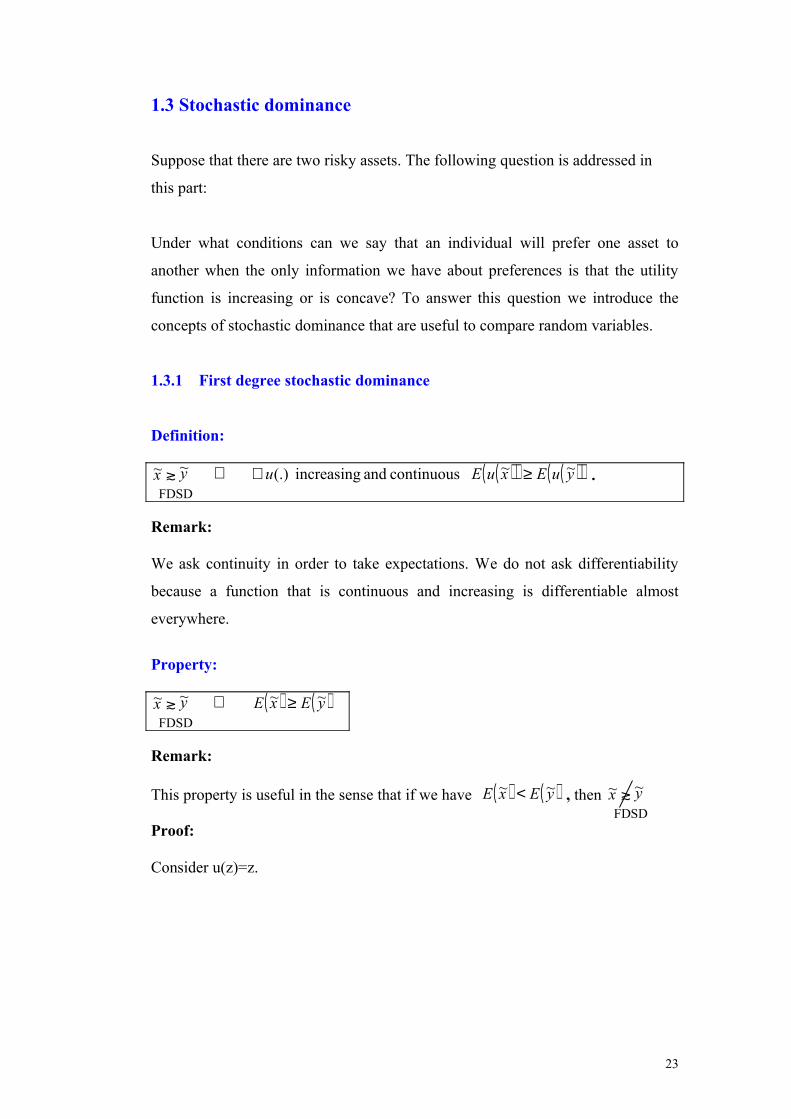
1.3 Stochastic dominance

Suppose that there are two risky assets. The following question is addressed in

this part:

Under what conditions can we say that an individual will prefer one asset to

another when the only information we have about preferences is that the utility

function is increasing or is concave? To answer this question we introduce the

concepts of stochastic dominance that are useful to compare random variables.

1.3.1 First degree stochastic dominance

Definition:

x~ ≳ y~ ⇔ ( )( ) ( )( ) ~~ continuous and increasing (.) yuExuEu ≥∀ . FDSD

Remark:

We ask continuity in order to take expectations. We do not ask differentiability

because a function that is continuous and increasing is differentiable almost

everywhere.

Property:

x~ ≳ y~ ⇒ ( ) ( ) ~~ yExE ≥ FDSD

Remark:

This property is useful in the sense that if we have ( ) ( ) ~~ yExE < , then x~ ≳ y~ FDSDProof:

Consider u(z)=z.

23

The opposite implication is not true in general. A counter-example is the following:

Characterizations:

Let ( ) ( )⋅⋅ yx FF and denote the cumulative distribution of x~ and y~ , respectively.

1. x~ ≳ y~ ⇔ ( ) ( ) [ ]a,bzFzF yx ∈∀≤ z , . FDSD

Intuition:

Proof:

24

2. x~ ≳ y~ ⇔ y~ d

= ε~~ +x , with 0~ ≤ε . FDSD

Proof:⇒ This part is omitted because is very technical.⇐ ( )( ) ( )( ) ( )( )xuExuEyuE ~~~~ ≤+= ε

1.3.2 Second degree stochastic dominance

Definition:

Properties:

Proof:

In particular,

( ) ( )

~~ )( yExEzzu ≥⇒=

( ) ( ) ( ) ( )

~~ ~~)( yExEyExEzzu ≤⇒−≥−⇒−=

( ) ( ) ( ) ( ) ( )

~var~var ~var~var)~()( 2 yxyxzEzzu ≤⇒−≥−⇒−−=

The opposite implication is not true. In the Laffont’s book there is a numerical counter-example:

25

x~ ≳ y~ ⇔ ( )( ) ( )( ) set) countable aon (except

~~ continuous is derivativefirst whoseconcave (.) yuExuEu ≥∀.

x~ ≳ y~ ≡ y~ is riskier than x~ in the Rothschild-Stiglitz sense SDSDS

≳ SDSD

x~ ≳ y~ ⇔ ( )( ) ( )( ) set) countable aon (except

~~ continuous is derivativefirst whoseconcave (.) yuExuEu ≥∀.

( ) ( )yExE ~~ =⇒

Characterizations:

Let ( ) ( )⋅⋅ yx FF and denote the cumulative distribution of x~ and y~ , respectively.

1. x~ ≳ y~ ⇔ i) ( ) ( )( ) [ ]a,b,dzzF zFt

a yx ∈∀≤−∫ t 0 .

SDSD ii) ( ) ( )( ) 0=−∫b

a yx dzzF zF

Intuition:

26

Proof:

27

2. x~ ≳ y~ ⇔ y~ d

= ε~~ +x , with ( ) 0~|~ =xE ε . SDSD

y~ is called a mean-preserving spread of x~ .

Intuition:

(If you add noise the new density is more disperse)

Proof:⇒ This part is omitted because is very technical.⇐

( )( ) ( )( ) ( )( )( ) ( )( )( ) ( )( ) ( )( )xuExuExxEuExxuEExuEyuExxx

~~~|~~~|~~~~~~~~~~ ==+≤+=+= εεε εε

1.3.3 Second degree stochastic monotonic dominance

Definition:

x~ ≳ y~ ⇔ ( )( ) ( )( ) ~~ concave and increasing (.) yuExuEu ≥∀ . SDSMD

Property:

x~ ≳ y~ ⇒ ( ) ( ) ~~ yExE ≥ SDSMD

Characterizations:

Let ( ) ( )⋅⋅ yx FF and denote the cumulative distribution of x~ and y~ , respectively.

1. x~ ≳ y~ ⇔ i) ( ) ( )( ) [ ]a,b,dzzF zFt

a yx ∈∀≤−∫ t 0 .

SDSMD ii) ( ) ( )( ) 0≤−∫b

a yx dzzF zF

2. x~ ≳ y~ ⇔ y~ d

= ε~~ +x , with ( ) 0~|~ ≤xE ε . SDSMD

28

Application of the concept of stochastic dominance to the simplest portfolio

selection problem (Rothschild and Stiglitz (1971))

Consider a risk averse investor with an initial wealth W0 to be invested in a risky

asset, asset 1, with a gross return 1

~R , and a riskless asset with a gross return fR .

Let A1 denote the optimal amount invested in the risky asset 1. Suppose that A1 is

characterized by the FOC, that is

( )( )( )( ) 0~~

' 1110 =−−+ fff RRARRWRuE .

Imagine now the following situation. There exists another risky asset, asset 2, that

is riskier than asset 1 in the Rothschild and Stiglitz sense, 1

~R ≳ 2

~R .

SDSD

Question:

If the same individual can invest in the risky asset 2 and the riskless asset, is he

going to invest less in the risky asset because now the risky asset is more risky?

Let A2 denote the optimal amount invested in the risky asset 2. Suppose that A2 is

characterized by the FOC, that is

( )( )( )( ) 0~~

' 2220 =−−+ fff RRARRWRuE .

Notice that a sufficient condition for having A2 ≤ A1 is

( )( )( )( ) ( )( )( )( )ffffff RRARRWRuERRARRWRuE −−+=≤−−+ 22202120

~~'0

~~' .

Let ( )( )( )fff RxARxWRuxg −−+= 10')( . If )(xg is concave, then this inequality

holds.

Exercise: Prove that ( ) ( ) ( )0 and 0,1 ≤≥≤

dx

xdR

dx

xdRxR AR

R implies that g is

concave.

29

A utility function that satisfies the tree conditions is

( ) .10 with , <<= σσ

σzzu

30