1 1. Facility Location 1.1 The Supply Chain Figure 1.1 shows a typical supply chain for a single plant. In the figure, items D and E provided by two different tier-two suppliers are shipped to a tier-one supplier where they are used to produce item B, units of which are then shipped to the plant. Similarly, items F and G are used to produce item C, which, along with B, are the two raw materials used to produce the finished good A. Units of A are shipped to distribution centers (DCs), from which they are delivered to the final customer. The number of units shown along each lane (or arc) in the figure is meant to indicate the typical size of each shipment; e.g., one of the reasons that a DC might be used is that it is cheaper to transport larger loads from the plant to the DC and then transport small loads to each customer as needed. 1.1.1 Logistics Network Design The design of a logistics network involves determining how to supply products to customers at the least cost while providing the desired level of service. The level of service can include both the time required for delivery to the customer and the availability of the product. Given the location of available transshipment points (e.g., ports and DCs), the design problem includes issues like selecting the best mode of transportation between each point in the network, the frequency and quantity of each shipment, and the amount of each product to be stored at each DC. The total cost of transportation and inventory is used to guide the design, subject to service level requirements. Inventory costs are the sum of cycle, in-transit, and safety stock inventory. Generally, there is a trade-off between transportation and inventory costs; e.g., transportation costs are lower for truckload shipments as compared to less-than-truckload, but they can increase cycle inventory costs while product waits for a full truckload to accumulate. In some cases, the design problem includes the need to select the best location for some of the DCs in the network. When location decisions are part of the design, it may be necessary to include the cost of constructing and operating each DC as part of the total cost along with the cost of transportation and inventory.
Transcript
1
1. Facility Location
1.1 The Supply Chain Figure 1.1 shows a typical supply chain for a single plant. In the figure, items D and E provided by two different tier-two suppliers are shipped to a tier-one supplier where they are used to produce item B, units of which are then shipped to the plant. Similarly, items F and G are used to produce item C, which, along with B, are the two raw materials used to produce the finished good A. Units of A are shipped to distribution centers (DCs), from which they are delivered to the final customer. The number of units shown along each lane (or arc) in the figure is meant to indicate the typical size of each shipment; e.g., one of the reasons that a DC might be used is that it is cheaper to transport larger loads from the plant to the DC and then transport small loads to each customer as needed.
1.1.1 Logistics Network Design The design of a logistics network involves determining how to supply products to customers at the least cost while providing the desired level of service. The level of service can include both the time required for delivery to the customer and the availability of the product. Given the location of available transshipment points (e.g., ports and DCs), the design problem includes issues like selecting the best mode of transportation between each point in the network, the frequency and quantity of each shipment, and the amount of each product to be stored at each DC. The total cost of transportation and inventory is used to guide the design, subject to service level requirements. Inventory costs are the sum of cycle, in-transit, and safety stock inventory. Generally, there is a trade-off between transportation and inventory costs; e.g., transportation costs are lower for truckload shipments as compared to less-than-truckload, but they can increase cycle inventory costs while product waits for a full truckload to accumulate. In some cases, the design problem includes the need to select the best location for some of the DCs in the network. When location decisions are part of the design, it may be necessary to include the cost of constructing and operating each DC as part of the total cost along with the cost of transportation and inventory.
1. FACILITY LOCATION
2
Figure 1.1. Typical logistics network for a plant.
As an example of a network design problem in the furniture industry, assume that a national furniture manufacturer has a large import program from suppliers in China. Currently, all products are shipped through the Panama Canal to a port on the East Coast and then trucked to a single DC. From there product is shipped to retail customers throughout the continental U.S. The manufacturer is considering whether a second DC should be opened at a predetermined location in California and used to receive product through the port of Long Beach. The second DC will decrease transportation costs from the DCs to the customers, but the sum of the inventory held both DCs will need to be greater because of loss of the opportunity at the single DC to pool safety stock inventory. Also, transport costs from China to Long Beach will be lower than the costs to the East Coast, but it may require than full container loads of low-volume products be shipped to each DC as compared to single container loads to the single DC, thereby doubling the cycle inventory levels of these products. Given all these factors, a network design decision can be made by determining the change in total logistics costs (transportation plus inventory costs) associated with opening the second DC.
DDDD
EEEE
FFFF
GGGG
CCCC
BBBB
AA
AA
A
A
A
A
Customers
DCsPlantTier OneSuppliers
Tier Two Suppliers
Resource
Market
vs.
vs.
vs.
vs.
Distribution Network
Distribution
Outbound Logistics
Finished Goods
Assembly Network
Procurement
Inbound Logistics
Raw Materials
downstream
upstream
A = B + C
B = D + E
C = F + G
1.1. THE SUPPLY CHAIN
3
Figure 1.2. Types of location problems.
1.1.2 Location Problems A taxonomy of the different types of location problems is shown in Figure 1.2. Cooperative location decisions are used to minimize the total system costs of multiple facilities owned by a single firm instead just minimizing the cost of each of the firm's individual facilities. These decisions are possible when the impact of the location of other firms’ facilities does not significantly impact the location of your facilities. Cooperative location problems that focus on optimizing something other than the sum of costs (e.g., minimizing the maximum cost) can be considered as “nonlinear” location problems because the location-related costs in these problems are not directly proportional to distance, as is the case in minisum problems. Competitive location decisions are used to minimize the cost of an individual facility with respect to other facilities owned by other firms. These decisions are required when the location of other firms’ facilities does impact the location of your facilities, and may result in sub-optimal decisions as compared to cooperative location decisions (cf. Hotelling’s law). In what follows, only transport-oriented minisum location problems are considered because these problems are the ones that most benefit from a simple analysis using transport-cost minimization as the sole criterion, and the assumption that costs are directly proportional to distance is usually reasonable; local-input-oriented location problem are typically solved using more complex multi-criteria-based approaches.
1.1.3 Basic Production System As shown in Figure 1.3, a production system can be considered as a node (or facility) in a logistics network that converts raw materials procured from suppliers into finished goods that are distributed to customers. For most production systems, the material input to the system equals
Location Decision
Cooperative Location
Competitive Location
Minisum Location“Nonlinear”
Location
Resource Oriented Location
Market Oriented Location
Transport Oriented Location
Local-Input Oriented Location
Minimax CostMaximin CostCenter of Gravity
Minimize Sum of Costs
Sum of Costs = SC = TC +LC
LC > TC
Local Input Costs = LC = labor costs, ubiquitous input costs, etc.
Minimize Individual Costs
PC > DC
Procurement Costs = PC
“Weight-losing” activities
DC > PC
Distribution Costs = DC
“Weight-gaining” activities
Minimize System Costs
TC > LC
Transport Costs = TC = PC + DC
1. FACILITY LOCATION
4
the material output from the system. Raw materials are those inputs that are transported to the production facility; ubiquitous inputs (e.g., water) are those available at any location, so that they do not need to be transported. Finished products are those outputs transported from the facility; while scrap is the output that is disposed of locally (although some outputs termed “scrap” are sometimes transported long distances from the facility for disposal or rework).
Figure 1.3. Basic production system.
The bottom portion of Figure 1.3 illustrates two different shipping terms that describe when the transfer of title occurs when goods are transported from the seller to the buyer: FOB Origin and FOB Destination, where FOB stands for free on board.1 In most cases, the cost of transporting the goods is paid for by whoever is the owner of the goods during the transport. Referring to Figure 1.3, assuming that you represent the production system, the supplier (the seller) would pay for the transport of goods from the supplier’s location (the origin) to your (the buyer’s) facility (the destination) if the shipping terms were FOB Destination.
1.2. SINGLE-FACILITY MINISUM LOCATION
5
1.2 Single-Facility Minisum Location Assuming that local input costs are either the same at every location or are insignificant as compared to transport costs, the minisum transport-oriented single-facility location problem is to locate a new facility (NF) to minimize the sum of weighted distances between NF and m existing facilities EFi, i = 1, …, m:
1 1
Min ( ) ( , ) ( , )im m
i i i i ii i
i
c
TC X w d X P q r d X Pw
(1.1)
where
wi = monetary weight ($/mile)
qi = physical weight (tons) or fi = physical weight rate (tons/year)
ri = transport rate ($/ton-mile)
d(X, Pi) = distance between NF at X and EFi at Pi (miles)
ci = unit cost ($/ton), used to determine qi after NF located (transportation problem)
X = location of new facility (NF)
Pi = location of existing facility i (EFi)
m = number of EFs
If physical weight qi is used, then TC in (1.1) is in units of $; if, instead, the physical weight rate fi in units of tons per year is used, then TC is in units of $/year.
1.2.1 Majority Theorem The Majority Theorem can be used to determine if one of the EFs has at least half of the total weight (i.e., a majority); if so, then the NF should be located at that EF in order to minimize TC:
Majority Theorem: Locate NF at EFj if 1
, where2
m
j ii
Ww W w
(1.2)
The theorem is true for all minisum problems with metric distances, and can used to as a first check before using other means of determining the optimal location for the NF.
1.2.2 Weight-Gaining vs. Weight-Losing Activities The activity occurring at a NF is considered weight losing if the sum of the monetary weights from EFs supplying material to the NF exceeds the sum of the weights of the material sent from the NF to the EFs which it supplies; conversely, if the sum of the monetary weight into the NF is less than the sum of the weight out, then the activity is considered weight gaining. In situations
1. FACILITY LOCATION
6
where the NF is a distribution center (DC), it is common for the products to be weight gaining because, while the physical weight of the products into the DC is the same as the weight of the products out, more costly modes of transport are used for distribution as compared to procurement, resulting in higher monetary weights on the outbound side of the DC (and thus drawing the location of the DC to the market).
1.2.3 Median Location Starting from the first EF, a median location is the first EF location at which the cumulative weight of the EFs up to that point is at least half of the total weight of all EFs (i.e., the EF location that splits the total weight into equal halves). The median location is the optimal NF location for all 1-D minisum problems and any 2-D rectilinear distance location problem.
The following procedure can be used to determine the median location:
Median location: For each dimension x of X:
1. Order EFs so that 1 2 mx x x
2. Locate x-dimension of NF at the first EFj where 1 1
, where2
j m
i ii i
Ww W w
If the cumulative weight at EFj exactly equals half of the total weight, then the optimal location along the x-dimension for the NF is any point between and including EFj and EF ( 1)j . Note that the optimal location for the NF can be determined without knowing the actual distances between the EFs; all that is necessary is to be able to order the EFs along each dimension.
For 2-D minisum problems other than rectilinear distance problems, then an iterative procedure must be used to optimize TC and thus determine the optimal location for a NF.
Figure 1.4. Total cost curve for 2 EFs.
3010
-8
+8
+5
-3
+2
-5+3
1 2
25 x
TC
90
+w1
+w2
+w1+w2
-w2
-w1
-w1-w2
+w1-w2
1.2. SINGLE-FACILITY MINISUM LOCATION
7
Figure 1.5. Total cost curve for 4 EFs.
Derivation
Figure 1.4 shows an example with two EFs. EF1 is located at x1 = 10 and has a weight of w1 = 5, while EF2 is located at x2 = 30 and has a weight of w2 = 3. The total cost of locating a single NF at x is the sum of the costs for each EF:
1 1 2 2, if
( ) ( ) ( ), where, if
i i
ii i
w x xTC x x x x x
w x x
For NF at x = 25,
1 2(25) (25 10) ( )(25 30)
5(15) ( 3)( 5) 90
TC w w
Figure 1.5 shows an example with four EFs, where only the total cost curve is shown. The slope of curve from – to x1 is
,11
m
ii
w W
and the slope between xj and xj+1 is
, 11 1
j m
j j i ii i j
w w
Starting at x1, the minimum total cost corresponds to the point where the slope of the total cost curve switches from negative to positive (or zero); this is equivalent to finding the first j such that
wi
-5-3-2-4 = -14 +5-3-2-4 = -4 +5+3+2-4 = +6
Minimum at point whereTC curve slope switchesfrom (-) to (+)
5
TC
3 2 4
1 2 3 4
-14
-4 +2+6
+14
+5+3-2-4 = +2 +5+3+2+4 = +14
5 < W/2 5+3=8 > W/2
4 < W/24+2=6 < W/24+2+3=9 > W/2
1. FACILITY LOCATION
8
1 1
1 1
1 1 1 1
1
1
0
2
2
j m
i ii i j
j m
i ii i j
j j j m
i i i ii i i i j
j
ii
j
ii
w w
w w
w w w w
w W
Ww
In Figure 1.5, W = 14 and W/2 = 7. Starting from either EF1 or EF4, the optimal solution is found at EF2, which corresponds to the location at which the median condition is first satisfied.
1-D Example
Problem: As shown in Figure 1.6, I-40 passes through Asheville, Statesville, Winston-Salem, Greensboro, Durham, Raleigh, and Wilmington. The number of road miles from the beginning of I-40 at the western border of North Carolina to each city is shown below its name. A company wants to build a facility along I-40 to serve customers located in these cities. If the weekly demand in truckloads of the customers in each city is 6, 4, 3, 2, 1, 3, and 5, respectively, determine where the facility should be located to minimize the distance traveled to serve the customers assuming that I-40 will be used for all travel.
Solution: Since W = 24, the cumulative weights at the optimal location should equal or exceed W/2 = 12, which occurs at Winston-Salem. Note that (1) the same solution is found starting from either Asheville or Wilmington, and (2) the distance between cities is not used to determine the optimal location, just the relative ordering the cities along I-40.
1.2. SINGLE-FACILITY MINISUM LOCATION
9
Figure 1.6. 1-D minisum location example.
2-D Example
Problem: A new snack machine is to be located on the floor of a facility (see Figure 1.7). Workers from eight different departments will make 19, 53, 82, 42, 9, 8, 39, and 6 trips per shift to the machine. Assuming rectilinear distance is a reasonable approximation of the actual travel distance, what is the location for the snack machine that will minimize the total distance that the workers have to travel?
Solution: A separate 1-D location problem can be solved for each dimension. Since W = 258, the cumulative weights at the optimal location should equal or exceed W/2 = 129. Along the bottom (x) dimension, the optimal location is at same x-location as departments 4 and 6, while along the left (y) dimension, the optimal location is anywhere between y-locations of departments 4 and 6. The optimal y-location is not a single point because the cumulative weight exactly equals 129, which corresponds to the total cost curve being flat between points 4 and 6. Note that the weights of departments at the same location are added together along each dimension.
1-D Example with Procurement and Distribution Costs
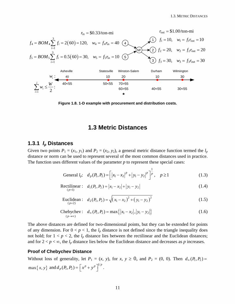
Problem: A product will be produced at a single plant that will be located along I-40 to serve customers located in the cities shown in Figure 1.6, above. Two tons of raw materials from a supplier in Asheville and a half ton of a raw material from a supplier in Durham are used to produce each ton of finished product that is shipped to customers in Statesville, Winston-Salem, and Wilmington. The demand of these customers is 10, 20, and 30 tons per year, respectively, and it costs $0.33 per ton-mile to ship raw materials to the plant and $1.00 per ton-mile to ship finished goods from the plant to the customers. Determine where the plant should be located so that procurement and distribution costs (i.e., the transportation costs to and from the plant) are minimized.
Solution: As shown in Figure 1.8, total customer demand is 60 tons per year, which translates into a demand of 120 tons per year based on a bill-of material (BOM) ratio of 2 for the supplier in Asheville and 30 tons per year based on a BOM of 0.5 for the supplier in Durham. The resulting monetary weights are used to determine that the plant should be located in Winston-Salem. The plant is (monetary) weight gaining since in out50 60w w , but the plant is physically weight losing since in out150 60f f ; the difference is due the higher outbound transport rate.
5 15 60 70 90
15
25
60
70
95
1
2
3
4
5
6
7
8
X
Y19
53
82
42
9
8
39
6
101101 < 129
50151 > 129157 > 129
*
48
107 < 129
53
59 < 129
6
6 < 129
Optimal location anywhere along line
: wi
: x
1.3. METRIC DISTANCES
11
Figure 1.8. 1-D example with procurement and distribution costs.
1.3 Metric Distances
1.3.1 lp Distances Given two points P1 = (x1, y1) and P2 = (x2, y2), a general metric distance function termed the lp distance or norm can be used to represent several of the most common distances used in practice. The function uses different values of the parameter p to represent these special cases:
General lp: 1
1 2 1 2 1 2( , ) , 1p p p
pd P P x x y y p (1.3)
( 1)
Rectilinearp
: 1 1 2 1 2 1 2( , )d P P x x y y (1.4)
( 2)
Euclideanp
: 2 22 1 2 1 2 1 2( , )d P P x x y y (1.5)
( )
Chebychevp
: 1 2 1 2 1 2( , ) max ,d P P x x y y (1.6)
The above distances are defined for two-dimensional points, but they can be extended for points of any dimension. For 0 < p < 1, the lp distance is not defined since the triangle inequality does not hold; for 1 < p < 2, the lp distance lies between the rectilinear and the Euclidean distances; and for 2 < p < , the lp distance lies below the Euclidean distance and decreases as p increases.
Proof of Chebychev Distance
Without loss of generality, let P1 = (x, y), for x, y 0, and P2 = (0, 0). Then 1 2( , )d P P
1.3.2 Great Circle (Geodesic) Distances Great circle, or geodesic, distances on the surface of a sphere (e.g., the earth (see Figure 1.9) correspond to the shortest distance between two points on the surface along the circle formed by the intersection of the surface and a plane passing through the center of the sphere (i.e., a “great circle”). The elevations of the points on the surface are usually ignored.
W0º Equator (0º lat)
Gre
enw
ich
(Prim
e)M
erid
ian
(0º
lon)
N
SE
North Pole (90ºN lat)
South Pole (90ºS lat)In
tern
atio
nal D
atel
ine
(180
º lon
)
Latit
ude
(y) Longitude (x)
(lon, lat) = (x, y)= (140ºW, 24ºN)= (–140º, 24º)
(Mer
idia
n)
(Parallel)
Figure 1.9. Longitude and latitude for points on the surface of the earth.
The great circle distance (dGC) between points 1 and 2 on the surface of the earth, specified by their longitude (lon) and latitude (lat) angles (in radians), is as follows:
1.3. METRIC DISTANCES
13
1 1 1 1 2 2 2 2
12 1 2 1 1 2
, , , , ,
great circle distance in radians of a sphere
cos sin sin cos cos cos
(radius of earth at equator) (bulge from north pole to equator)
3,963.34 13.35 s
rad
lon lat x y lon lat x y
d
y y y y x x
R
1 2 1 2
GC 1 1 2 2
in mi, 6,378.388 21.476 sin km2 2
distance , to , rad
y y y y
d x y x y d R
To convert between decimal degrees and radians: deg radrad deg
180and
180
x xx x
To convert degrees (DD:MM:SS) to decimal degrees: deg
, if or 60 3,600
, if or 60 3,600
MM SSDD E N
xMM SS
DD W S
Example
Table 1.1 shows a spreadsheet that calculates the great circle distance from Raleigh, NC to Gainesville, FL, Baghdad, Iraq, and Rio de Janeiro, Brazil. There are typically slight differences in great circle distance calculations due to how accurately the radius of the earth, R, is determined.
Table 1.1. Great Circle Distances from Raleigh
Circuity Factor
Since the great circle distance is usually less than the actual road (or rail) distance between any two locations, the great circle distance can be multiplied by a circuity factor k to approximate the actual road distance:
Actual road distance between P1 and P2 1 2( , )GCk d P P
The circuity factor is the average ratio of the actual road distance between two points and the great circle distance between the two points. It can be used to increase the easy-to-determine great circle distance so that it approximates the harder-to-determine actual road distance. You can use the websites How far is it or Google Maps to determine the great circle distances and the latter to determine road distances.
dd mm ss x (deg) x (rad) dd mm ss y (deg) y (rad) d(rad) d (mi)
Raleigh 78 39 32 W -78.659 -1.373 35 49 19 N 35.8219 0.6252
Gainesville 82 20 11 W -82.336 -1.437 29 40 27 N 29.6742 0.5179 0.12 475.0745Baghdad 44 22 E 44.3667 0.7743 33 14 N 33.2333 0.58 1.62 6407.166
Rio de Janeiro 43 12 W -43.2 -0.754 22 57 S -22.95 -0.401 1.181 4679.089
1. FACILITY LOCATION
14
Circuity factors of 1.15 to 1.25 are typically used for long-distance (> 20 mile) approximations, while factors of 1.25 to 1.50 are typically used for short-distance road approximations and for rail networks because the networks are not as dense. A factor of 1.20 provides a reasonable long-distance road approximation for the continental U.S.
Derivation
In Figure 1.10, a, b, and c are the sides of a spherical triangle and A, B, and C are the corresponding angles. The great circle distance between points 1 and 2 in radians (drad) corresponds to side c of the triangle.
Given
2 1 1 290 , 90 ,a y b y C x x
the formula for great circle distances can be derived using the spherical law of cosines for sides:
2 1 2 1 1 2
2 1 2 1 1 2
cos( ) cos( ) cos( ) sin( )sin( )cos( )
cos(90 )cos(90 ) sin(90 )sin(90 )cos( )
sin( )sin( ) cos( ) cos( ) cos( )
c a b a b C
y y y y x x
y y y y x x
(x2,y2)
(x1,y1)
B
C
A
a
c
b
North Pole
Prime
lon2= x2
lon 1= x 1la
t 2 =
y2
la t1 = y
1
Equator
Meridian
Figure 1.10. Great circle distance derivation.
Solving for c:
12 1 2 1 1 2cos sin( )sin( ) cos( ) cos( ) cos( )radd c y y y y x x
The above formula can result in round off error if the two points are located at exactly opposite sides of a sphere. Instead, the Haversine formula can be used:2\
1 2 1 21 2 21 22sin min 1, sin cos( ) cos( )sin
2 2rad
y y x xd c y y
The Haversine formula does not need to be used if the great circle distance is being calculated by hand and the two points are known to not be on opposite sides of the sphere.
1.4. MULTIFACILITY LOCATION
15
1.4 Multifacility Location In a multifacility location problem, the number of NFs to be located can either be specified or can be determined as part of the location procedure. When the number of NFs is specified, the allocation of EFs to NFs can either be given or determined as part of what is then termed a location–allocation problem. If the NF-to-EF allocations are given and there are no interactions between the NFs, then the multifacility problem reduces to a series of single-facility location problems. The location–allocation problem remains difficult even when there are no interactions between the NFs because of the need to determine the allocations.
Determining the best retail warehouse locations is an example of a location–allocation problem, where the EFs are population centroids (e.g., ZIP codes). Table 1.2 lists the best locations for a given number of warehouses. It is assumed that the warehouses serve retail customers located throughout the continental U.S. in proportion to population. Trucks traveling at 400 miles per day are used for all transport. Only outbound transport costs are used in making the location decision; it is reasonable to ignore inbound transport as long as suppliers are located uniformly throughout the country so that the inbound transport costs to each warehouse is approximately the same at any location. As can be seen in the table, the best single warehouse location (Bloomington, Indiana) is not the best location as the number of warehouses increases, while the warehouse in Palmdale, California remains in the best west coast location until a second west coast warehouse in Tacoma, Washington is added as part of the five-warehouse solution.
Table 1.2. Best Retail Warehouse Locations3
Number of Locations
Average TransitTime (days) Warehouse Location
1 2.20 Bloomington, IN 2 1.48 Ashland, KY Palmdale, CA 3 1.29 Allentown, PA Palmdale, CA McKenzie, TN 4 1.20 Edison, NJ Palmdale; CA Chicago, IL Meridian, MS 5 1.13 Madison, NJ Palmdale, CA Chicago, IL Dallas, TX Macon, GA 6 1.08 Madison, NJ Pasadena, CA Chicago, IL Dallas, TX Macon, GA Tacoma, WA 7 1.07 Madison, NJ Pasadena, CA Chicago, IL Dallas, TX Gainesville, GA Tacoma, WA Lakeland, FL 8 1.05 Madison, NJ Pasadena, CA Chicago, IL Dallas, TX Gainesville, GA Tacoma, WA Lakeland, FL Denver, CO 9 1.04 Madison, NJ Alhambra, CA Chicago, IL Dallas, TX Gainesville, GA Tacoma, WA Lakeland. FL Denver, CO Oakland, CA
10 1.04 Newark, NJ Alhambra, CA Rockford, IL Palistine, TX Gainesville, GA Tacoma, WA Lakeland, FL Denver, CO Oakland. CA Mansfield, OH
1. FACILITY LOCATION
16
1.4.1 The Uncapacitated Facility Location Problem Given m EFs and n sites at which NFs can be established, the uncapacitated facility location (UFL) problem can be formulated as the following mixed-integer linear programming (MILP) problem:
1 1 1
Minn n m
i i ij iji i j
TC k y c x
(1.7)
subject to
1
1n
iji
x
, 1, ,j m (1.8)
i ijy x , 1, , ; 1, ,i n j m (1.9)
0 1ijx , 1, , ; 1, ,i n j m (1.10)
0,1iy , 1, ,i n , (1.11)
where
ki = fixed cost of establishing a NF at site i
cij = variable cost to serve all of EF j’s demand from site i
yi = 1, if NF established at site i; 0, otherwise
xij = fraction of EF j’s demand served from NF at site i.
The UFL problem is a MILP because the yi’s are binary variables and the xij’s are real variables. In the UFL problem, all xij are 0 or 1; in the capacitated facility location (CFL) problem, there is a maximum capacity associated with each site, resulting in a xij value between 0 and 1 whenever not all of an EF j’s demand can be served from the NF at site j.
The MILP for the UFL problem is termed the “strong formulation” due to constraints (1.9), which results in an LP relaxation that gives a tight lower bound. When nm constraints (1.9) are replaced with the n constraints
1
m
i ijj
m y x
, 1, ,i n , (1.12)
the formulation is termed “weak” since the lower bound from the LP relaxation is not very tight, resulting in a large branch-and-bound tree.
Example
Given n = 6 sites, m = 6 EFs, and fixed and variable costs
1.4. MULTIFACILITY LOCATION
17
8 0 3 7 10 6 48 3 0 4 7 6 7
10 7 4 0 3 6 8;
8 10 7 3 0 7 89 6 6 6 7 0 28 4 7 8 8 2 0
i ijk c
,
the optimal solution is to establish two NFs at sites 3 and 6 serving EFs 2–4 and EFs 1, 5, and 6, respectively, for a TC = 31:
0 0 0 0 0 0 00 0 0 0 0 0 01 0 1 1 1 0 0
;0 0 0 0 0 0 00 0 0 0 0 0 01 1 0 0 0 1 1
i ijy x
.
1.4.2 The p-Median Problem When the number of NFs is specified and all of fixed costs are identical (or not stated), then the fixed costs will have no impact on the location decision and can be set to zero in (1.7) and the following constraint can be added to the UFL problem to formulate the p-median problem:
1
n
ii
y p
, (1.13)
where p is the number of NFs to be located. If non-identical fixed are included, then the p-median problem generalizes to the p-UFL problem, where both p-median and UFL are special cases.4
1. FACILITY LOCATION
18
1.5 References The following sources are recommended for further study:
Ahuja, R.K., Magnanti, T.L., and Orlin, J.B., 1993, Network Flows: Theory, Algorithms, and Applications, Englewood Cliffs, NJ: Prentice-Hall.
Mirchandani, P.B., and Francis, R.L., Eds., 1990, Discrete Location Theory, New York: Wiley.
Simchi-Levi, D., Kaminsky, P., and Simchi-Levi, E., 2008, Designing and Managing the Supply Chain: Concepts, Strategies, and Case Studies, 3rd Ed., Boston: McGraw-Hill.
Notes 1 What are FOB shipping terms? http://simplestudies.com/what-are-fob-shipping-terms.html (accessed Jan 2012). 2 Sinnott, R.W., 1984, “Virtues of the Haversine”, Sky and Telescope 68(2):159, as reported in http://www.census.gov/cgi-bin/geo/gisfaq?Q5.1 3 Table is adapted from Inbound Logistics, Oct. 2004, p. 50. 4 Krarup, J., and Pruzan, P.M., “Ingredients of locational analysis,” in Mirchandani, P.B., and Francis, R.L., Eds., 1990, Discrete Location Theory, New York: Wiley, p. 20.
1
Facility Location–Allocation Problem
Location–Allocation (LA) Problem: Determine both the location of n new facilities (NFs) and the allocation of the flow requirements of m existing facilities (EFs) to the NFs that minimize total transportation costs.
Continuous: Minimize 1 1
, ( , )m n
ji j ii j
f X W w d X P
subject to 1
, 1, ,n
ji ij
w w i m
0, 1, , ; 1, ,jiw j n i m
where X = , , 1, ,j j jX x y j n , NF locations
W = , 1, , ; 1, ,jiw j n i m , allocated flow requirements
Pi = ,i ia b , location of EF i
( , )j id X P = distance between NF j and EF i
wi = flow requirement of EF i
Since there are no capacity constraints on the NFs, optimal solutions lie at extreme points of the constraint set of the nonlinear programming (Continuous) formulation of LA problem, i.e.,
wki = wi, for j = k, and wji = 0, for j k,
allocated flow requirements W can be replaced by the allocation vector
, 1, , , and 1, ,i ii m n
resulting in a mixed continuous–combinatorial formulation:
Mixed: Minimize 1
, ( , )i
m
i ii
f X w d X P
If there were constraints on the maximum flow capacity of the NFs, then more than one wji could be nonzero in an optimal solution and W could not be replaced by the allocation vector .
2
0 1 2 3 4 5 6 7 8 9 10
0
1
2
3
4
5
6
7
8
9
10
EF1
EF2 EF3
EF4
EF5
EF6
EF7
EF8
EF9
NF1
NF2
NF3
x−axis
y−ax
is
Final NF Locations (9 EFs and 3 NFs)
Figure 1. 9-EF by 3-NF location–allocation problem instance.
NF locations: 1.7, 1.3 , 3.4, 9.3 , 8.0, 5.5X
Allocation vector: 1 3 1 3 1 1 3 3 2
Total transportation cost: ,f X = 11.78
Euclidean distances: 2 2,i i ii i id X P x a y b
Flow requirements: All wi = 1
Number of feasible allocations: 9
3,0253
mn
Alternate Location–Allocation (ALA) Procedure Given initial NF locations, ALA local improvement procedure finds optimal EF allocations and then finds optimal NF locations for these allocations, continuing to alternate until no further EF allocation changes are made. Introduced by Cooper in 1963, ALA is still the best heuristic for the LA problem. Since the ALA procedure finds only a local optima, the procedure should be applied multiple times using different initial NF locations, keeping the best solution found as the final solution. This type of repeated application of a local improvement procedure is termed a multistart metaheuristic.
3
0 2 4 6 8
0
1
2
3
4
5 EF1 EF2
EF3
EF4 EF5
EF6 EF7
NF1
NF2
x−axis
y−ax
is
Initial NF Locations (Obj. value = 27)
0 2 4 6 8
0
1
2
3
4
5 EF1 EF2
EF3
EF4 EF5
EF6 EF7
NF1
NF2
x−axis
y−ax
is
Second NF Locations (Obj. value = 20)
0 2 4 6 8
0
1
2
3
4
5 EF1 EF2
EF3
EF4 EF5
EF6 EF7
NF1
NF2
x−axis
y−ax
is
Final NF Locations (Obj. value = 18)
Figure 2. ALA procedure for 7-EF by 2-NF problem instance
ALA PROCEDURE: , , ,X ALA X P w
1. Given initial NF locations X
2. TC
3. ,allocate X P
4. , ,X locate P w
5. If ,TC X TC , stop; otherwise ,TC TC X , X X , , and go to step 3
4
LOCATION PROCEDURE:
Solve n single-facility location problems using the EFs allocated to each NF
Exact O(m) procedure for rectilinear distances (median conditions)
Iterative procedure for general lp distances—in MATLAB, quasi-Newton followed by Nelder-Mead simplex
ALLOCATION PROCEDURE:
Allocate each EF to its closest NF
If NFs were capacitated, then would have to solve a minimum cost network flow problem to perform the allocation, where each EF might be allocated to more than one NF
Solution Space of LA Problem Mix of continuous and combinatorial
Continuous: X
2n-dimensional space of NF locations: 1 1, , , ,n nX x y x y
Combinatorial:
1
1( 1)
!
nn j m
j
m nj
n jn
feasible allocations of n NFs to m EFs
Although nm allocations are possible, since NFs are indistinguishable:
Number of feasible allocations = number of ways m distinguishable EFs can be allocated to n indistinguishable NFs, with each NF allocated to at least one EF