52
1 Further Maths Chapter 4 Displaying and describing relationships between two variables
| Date post: | 01-Jan-2016 |
| Category: |
Documents |
| Upload: | brandon-lambert |
| View: | 218 times |
| Download: | 0 times |

1
Further Maths
Chapter 4Displaying and describing
relationships between two variables
2
Bivariate Data
• Often we are interested to see if a relationship exists between two variables, i.e. – Hours studied and study score, – Gender and resting pulse rate– Hair colour and Favourite Sport
3
Dependent and Independent Variable
• The first thing that needs to be considered is if there is some sort of dependency relationship between the two i.e. which of the two variables is likely to depend on the other?
• Does a person’s study score depend on number of hours studied or does the number of hours a person studies depend on their study score?
• Complete the other examples
4
Dependent and Independent Variable
• In the first case, the study score is the dependent variable, hours studied is the independent variable.
• In the second case, the resting pulse rate is the dependent variable, gender is the independent variable
• In the third case you would not expect there to be any relationship

5
Dependent and Independent Variable
• The variable that can be controlled is referred to as the independent variable. The variable that is measured in response is referred to as the dependent variable.
6
3 possible cases
• There are three possible situations that may occur when considering two variables at the one time
• Both variables are categorical • One variable is categorical and the other is
numerical • Both variables are numerical
7
Categorical and Categorical
• One hundred people were randomly selected and surveyed as to whether they were in favour of lowering the speed limit in suburban streets to 40 km/h.

8
Categorical and Categorical
• When the data was tabulated it was found that from the males interviewed, 25 were in favour and the rest against. Of the females, 20 were in favour and the rest against.
9
Categorical and Categorical
• The group consisted of 65 males and 35 females. Each person voted for or against the proposal.
• The independent variable is• The dependent variable is
10
Categorical and Categorical
• A two way frequency table is an appropriate way to display this data
• The independent variable should be put in the columns.
• The dependent variable should be put in the rows.

11
Categorical and Categorical
Gender
Male Female
Opi
In favour
niOn
Not in favour
Total

12
Categorical and Categorical
Gender
Male Female
Opi
In favour
25 20
nion
Not in favour
40 15
Total 65 35

13
Categorical and Categorical
• Does this table appear to indicate that men are more in favour of lowering the speed limit than women?
• Discuss
14
Categorical and Categorical
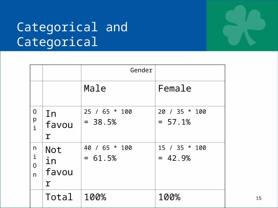
• Two way frequency table (appropriately percentaged)
• Since the independent variable is in the columns, we need to calculate column percentages.
15
Categorical and Categorical
Gender
Male Female
Opi
In favour
25 / 65 * 100
= 38.5%20 / 35 * 100
= 57.1%
niOn
Not in favour
40 / 65 * 100
= 61.5%15 / 35 * 100
= 42.9%
Total 100% 100%

16
Categorical and Categorical
• This can then be displayed using a percentaged segmented barchart.

17
Should the speed limit be lowered ?
0%
10%
20%
30%
40%
50%
60%
70%
80%
90%
100%
Male Female
Gender
Perc
enta
ge Not in favour
In favour

18
Categorical and Categorical
• Report• 57.1% of females are in favour of lowering the
speed limit compared to 38.5 % of men. Women are clearly more in favour of lowering the speed limit.
19
Exercises
• Exercise 4A Pages 88 – 89 all• Exercise 4B Page 91 all

20
Numerical and Categorical
• An investigation was carried out to see if there was a relationship between gender and resting pulse rate.
• Data was collected of the resting pulse rates of 23 boys and 23 girls.Dependent variable isIndependent variable isNumerical variable isCategorical variable is
Pulse rate
Gender
Pulse rate
Gender

21
Numerical and Categorical
• Males 80 73 73 78 75 6970 70 78 58 77 64
76 67 69 72 71 6872 67 77 73 65
Females 65 73 74 81 59 6476 83 95 70 73 79
64 77 80 82 7787 66 89 68 78 74
22
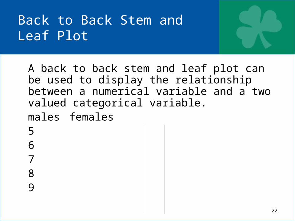
Back to Back Stem and Leaf Plot
A back to back stem and leaf plot can be used to display the relationship between a numerical variable and a two valued categorical variable.
males females56789

23
Parallel Boxplots
• Parallel box plots can be used to display the relationship between a numerical variable and a two or more level categorical variable.
• Calculator Display
• Exercise 4C Page 93 Questions 1-3
24
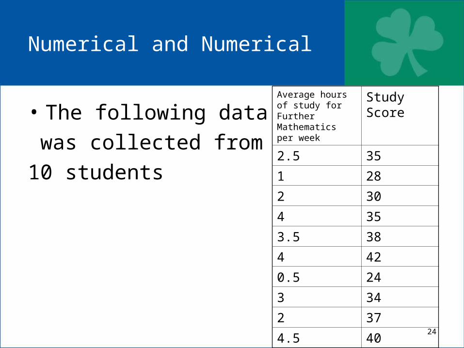
Numerical and Numerical
• The following data was collected from 10 students
Average hours of study for Further Mathematics per week
Study Score
2.5 35
1 28
2 30
4 35
3.5 38
4 42
0.5 24
3 34
2 37
4.5 40
25
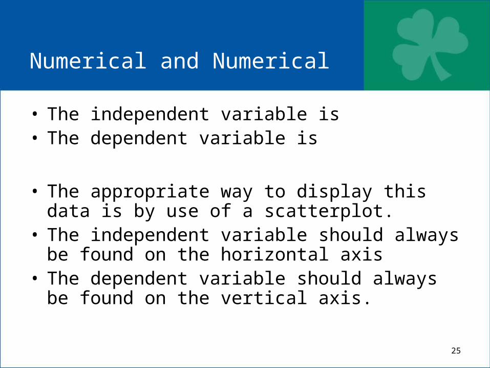
Numerical and Numerical
• The independent variable is• The dependent variable is
• The appropriate way to display this data is by use of a scatterplot.
• The independent variable should always be found on the horizontal axis
• The dependent variable should always be found on the vertical axis.

26

27
Calculator
• Calculator Display• Exercise 4D Page 96 all

28
Interpreting a Scatterplot
• When describing a scatterplot the following four features should be discussed
• Direction• Form• Strength• Outliers
29
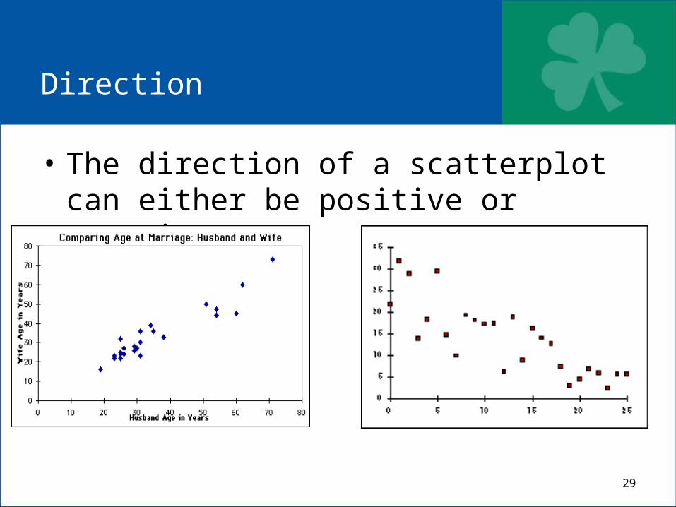
Direction
• The direction of a scatterplot can either be positive or negative
•

30
Form
• The form of a scatterplot can either be linear or non-linear
31
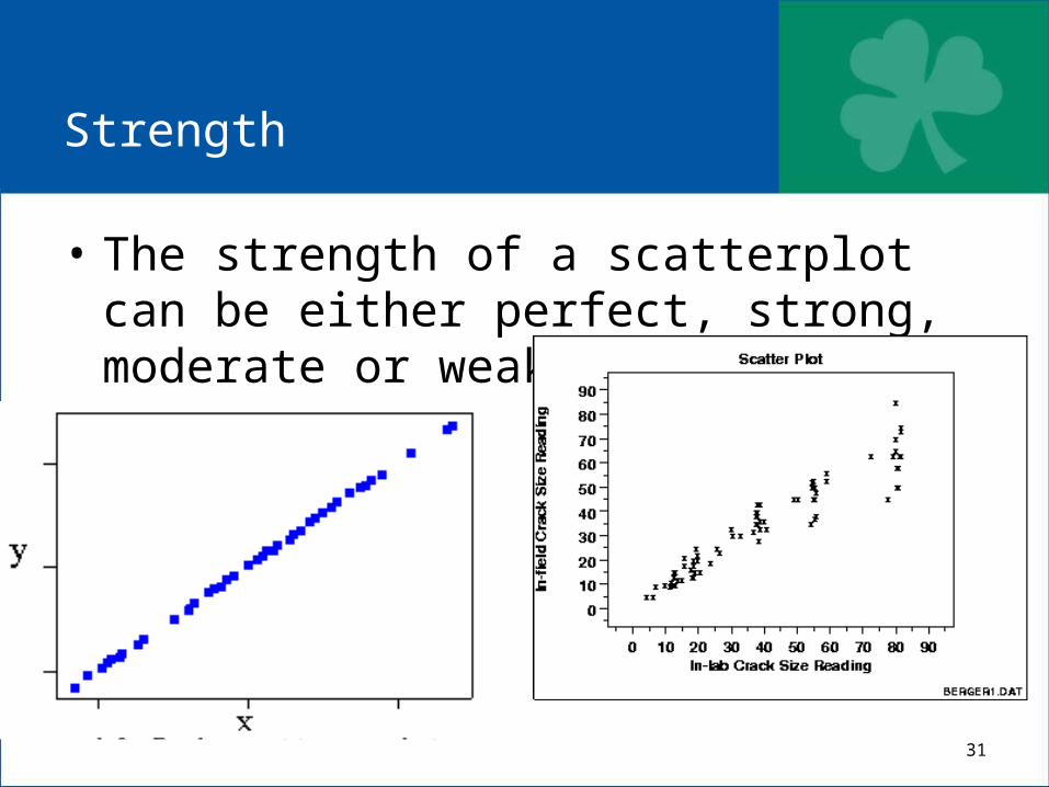
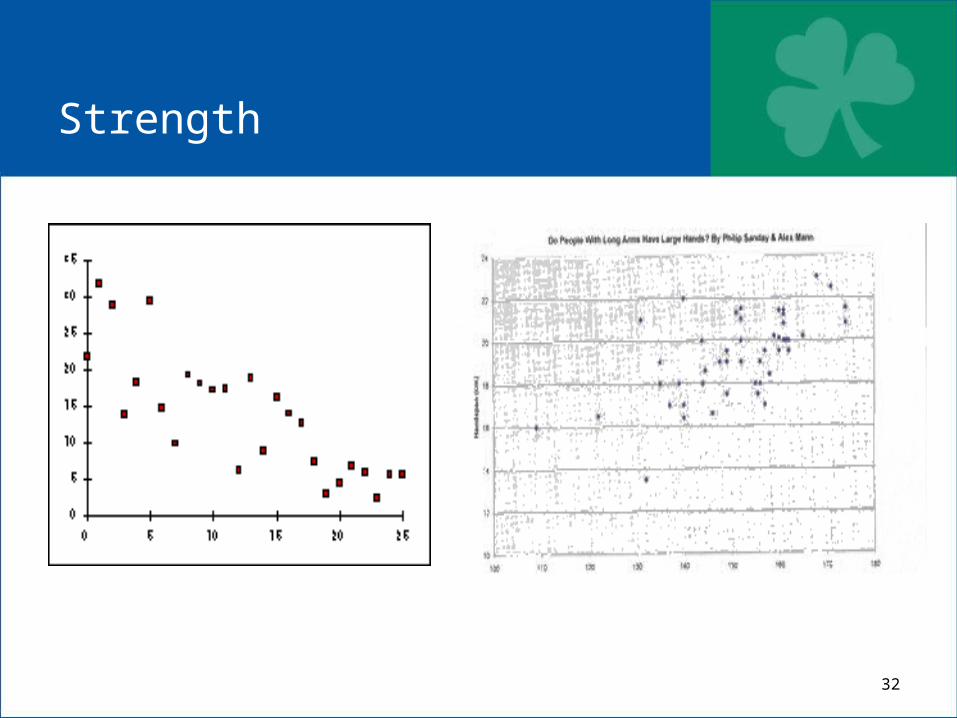
Strength
• The strength of a scatterplot can be either perfect, strong, moderate or weak.
32
Strength

33
Outliers
• Outliers are any points that are separated from the general body of points
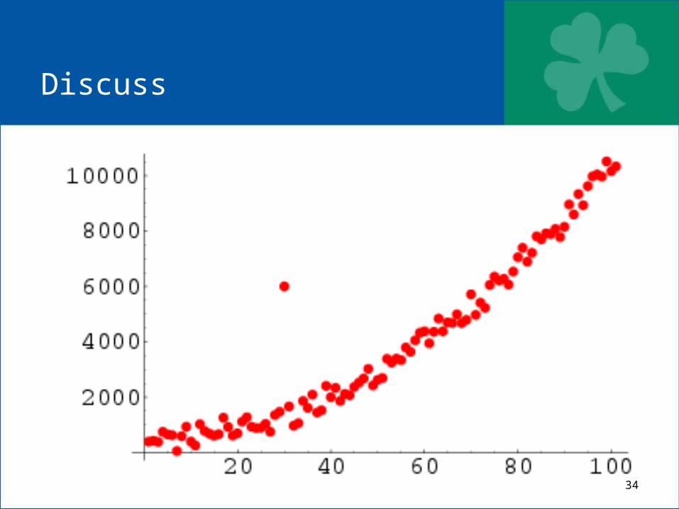
34
Discuss
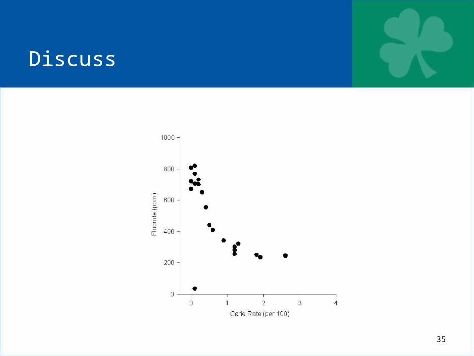
35
Discuss

36
Discuss
37
Correlation coefficient (r)
• r is a measure of the strength of the linear relationship between two numerical variables. The value of r is between –1 (perfect negative linear relationship) and
1 (perfect positive linear relationship).• It is not appropriate to calculate a correlation
coefficient if there are outliers in the data.
38
Estimating r
• Board Work• Exercise 4E Page 100-101 all
39
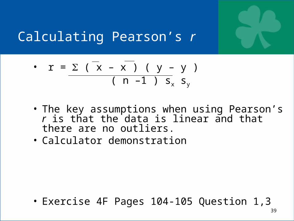
Calculating Pearson’s r
• r = ( x – x ) ( y – y ) ( n –1 ) sx sy
• The key assumptions when using Pearson’s r is that the data is linear and that there are no outliers.
• Calculator demonstration
• Exercise 4F Pages 104-105 Question 1,3
40
Coefficient of Determination (r2)
• The coefficient of determination is the square of Pearson’s correlation coefficient.
• It is used to explain the degree to which one variable can be predicted from another variable
41
Coefficient of determination
• The coefficient of determination gives the percentage variation (r2 * 100) in the dependent variable that is explained by the variation in the independent variable.
42
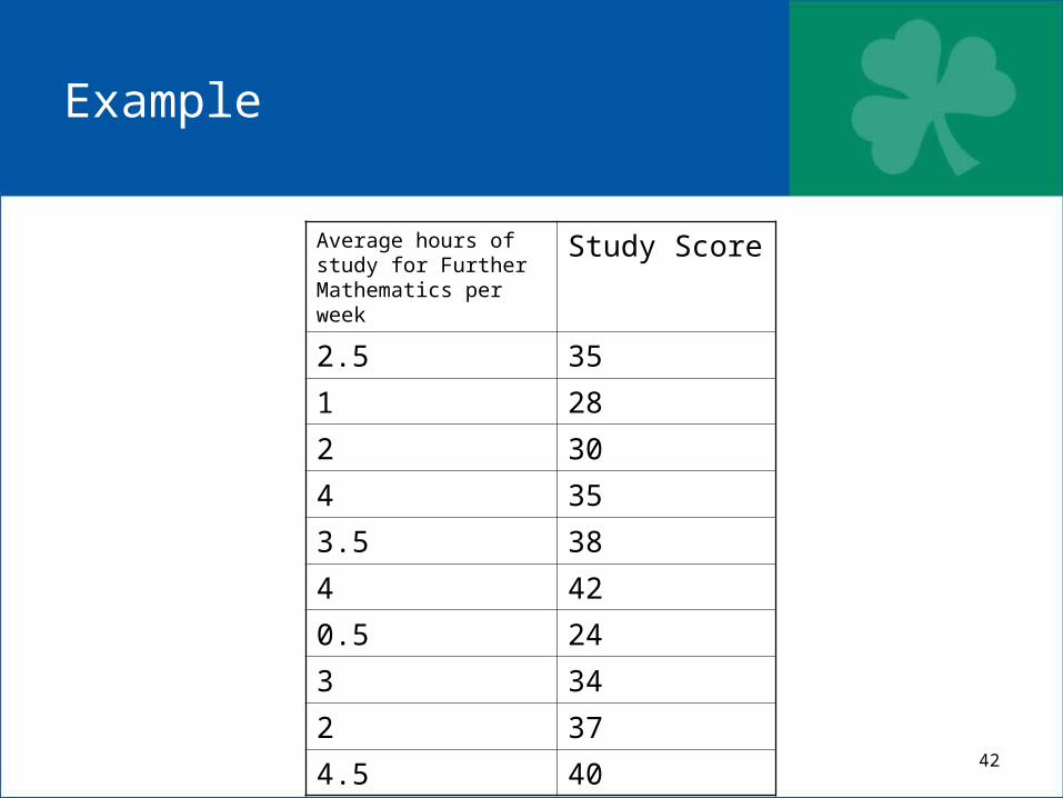
Example
Average hours of study for Further Mathematics per week
Study Score
2.5 35
1 28
2 30
4 35
3.5 38
4 42
0.5 24
3 34
2 37
4.5 40
43
Example
• Calculate r and interpret• Calculate r2
• Interpret r2
44
Example
• of the variation in the study score can be explained by the variation in the number of hours studied per week. The other is due to other factors.
45
Warning
• Pearsons r can be positive or negative depending on the direction of the scatterplot.
• The coefficient of determination will always be positive and is normally expressed as a percentage.
46
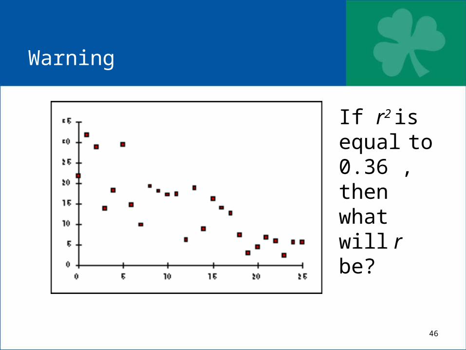
Warning
If r2 is equal to 0.36 , then what will r be?
47
Exercise
• Complete Exercise 4G Pages 107-108 all
48
Correlation and Causation
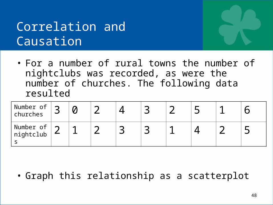
• For a number of rural towns the number of nightclubs was recorded, as were the number of churches. The following data resulted
• Graph this relationship as a scatterplot
Number of churches 3 0 2 4 3 2 5 1 6Number of nightclubs 2 1 2 3 3 1 4 2 5

49
Correlation and Causation
0
1
2
3
4
5
6
0 1 2 3 4 5 6 7
Number of churches
Nu
mbe
r o
f n
igh
tclu
bs
50
Correlation and Causation
• Interpret this graph.
• As the number of churches increases, so does the number of nightclubs.
• Therefore an increase in the number of churches will lead to or cause an increase in the number of nightclubs.
• As people become more religious they will tend to visit nightclubs more.
• Nightclubs will be full of super religious people.

51
Correlation and Causation
• An increase in one variable will not always cause an increase in the other. In this situation there is a third variable that is hidden
• I.e. Population • Therefore we never use the word cause when
describing a relationship.• We say • As the number of churches increases, the number of
nightclubs tends to increase.• Exercise 4H Page 108 – 109 all
52
Chapter 4
• Exercise 4I Page 109


