1

Heat Transfer in Microchannels

11.1 Introduction:

Applications

Micro-electro-mechanical systems (MEMS): Micro heat exchangers, mixers, pumps, turbines, sensors and actuators

Cooling of microelectronics

Inkjet printer

Medical research

2

11.1.1 Continuum and Thermodynamic Equilibrium Hypothesis

Properties: (pressure, temperature, density, etc) are macroscopic manifestation of molecular activity

Continuum: material having sufficiently large number of molecules in a given volume to give unique values for properties

Validity of continuum assumption: the molecular-mean-free path, , is small relative to the characteristic dimension of the system

Mean-free-path: average distance traveled by molecules before colliding

3

Knudson number Kn:

eDKn

(1.2)

eD = characteristic length

Gases: the criterion for the validity of the continuum assumption is:

110Kn (1.3a)

Thermodynamic equilibrium: depends on collisions frequency of molecules. The condition for thermodynamic equilibrium is:

310Kn (1.3b)

4

At thermodynamic equilbirium:fluid and an adjacent surface have the same velocity and temperature:

no-velocity slipno-temperature jump

Continuity, Navier-Stokes equations, and energy equation

are valid as long as the continuum assuption is valid

No-velocity slip and no-temperature jump

are valid as long as thermodynamic equilibrium is justified

Microchannels: Channels where the continuum assumptionand/or thermodynamic equilibrium break down

5

9.1.2. Surface Forces. Examine ratio of surface to volume for tube:

D/LD

DL

V

A 4

42

(11.1)

For D = 1 m, A/V = 4 (1/m)

For D = 1 μm, A/V = 4 x 10 6 (1/m)

Consequence: (1) Surface forces may alter the nature of surface boundary conditions

(2) For gas flow, increased pressure drop results in large density changes. Compressibility becomes important

6

9.1.3 Chapter Scope

Classification

Gases vs. liquids

Surface boundary conditions

Heat transfer in Couette flow

Heat transfer in Poiseuille flow

9.2 Basic Consideration

9.2.1 Mean Free Path. For gases:

RTp 2

(11.2)

7

p = pressure

NOTE:

Pressure drops along a channel increases

Kn increases

m610

is very small, expressed in terms of the micrometer, •

R = gas constant

T = temperature

μ = viscosity

Table 11.1

gas

Air

Helium

Hydrogen

NitrogenOxygen

R

2077.1

4124.3

296.8259.8

287.0

3kg/mKJ/kg mkg/s

m

1614.1

2840.1

1233.1

0808.0

1625.0

2.207

6.184

0.199

6.89

2.17807155.006577.0

1233.0

1943.0

067.0

710

values of for common gases

8

11.2.2 Why Microchannels?

Nusselt number: fully developed flow through tubes at uniformsurface temperature

66.3k

hDNuD (6.57)

D

kh 657.3 (11.3)

As D h

Application:

Water cooled microchips

010 110

110210

210

310

310

410

410

510

610

Fig. 11.1

m)(D

continuum

air

water

Fig. 11.2

flow

sink

microchip q

9

11.2.3 Classification

Based on the Knudsen number:

flowmolecularfreeKn

flowtransitionKn

flowslipcontinuumKn

flowslipnocontinuumKn

10

101.0

,1.0001.0

,001.0

(11.4)

Four important factors:

(1) Continuum

(2) Thermodynamic equilibrium

(3) Velocity slip

(4) Temperature jump

10

(1) Kn < 0.001: Macro-scale regime (previous chapters):

Continuum: valid

(2) 0.001 < Kn < 0.1: Slip flow regime:

Continuum: valid

Thermodynamic equilibrium: valid

No velocity slip

No temperature jump

Thermodynamic equilibrium: fails• Velocity slip • Temperature jump

Continuity, Navier-Stokes equations, and energy equations are validNo-velocity slip and No-temperature jump conditions, conditions fail

Reformulate boundary conditions

11

(3) 0.1< Kn<10: Transition flow:

(4) Kn>10: Free molecular flow: analysis by kinetic theory of gases

11.2.4 Macro and Microchannels

Macrochannels: Continuum domain, no velocity slip, no temperature jumpMicrochannels: Temperature jump and velocity slip, with or without failure of continuum assumption

Continuity and thermodynamic equilibrium fail Reformulate governing equations and boundary conditions

Analysis by statistical methods

12

Distinguishing factors:

(1) Two and three dimensional effects

(2) Axial conduction

(3) Viscous dissipation

(4) Compressibility

(5) Temperature dependent properties

(6) Slip velocity and temperature

(7) Dominant role of surface forces

13

11.2.5 Gases vs. Liquids

Macro convection:

No distinction between gases and liquids Solutions for both are the same for the same geometry, governing parameters (Re, Pr, Gr,…) and boundary conditions

Micro convection:

Flow and heat transfer of gases differ from liquids

Gas and liquid characteristics:

(1) Mean free path: gasliquid Continuum assumption may hold for liquids but fail for gases

14

Typical MEMS applications: continuum assumption is valid for liquids

(2) Knudsen number: used as criterion for thermodynamic equilibrium and continuum for gases but not for liquids

(3) Onset of failure of thermodynamic equilibrium and continuum: not well defined for liquids

(4) Surface forces: liquid forces are different from gas forces

(5) Boundary conditions: differ for liquids from gases

(6) Compressibility: liquids are almost incompressible while gases are not

(7) Flow physics: liquid flow is not well known. Gas flow is well known

15

(8) Analysis: more complex for liquids than gases

11.3 General Features

Flow and heat transfer phenomena change as channel size is reduced:

Rarefaction: Knudsen number effect

Compressibility: Effect of density change due to pressure drop along channel

Viscous dissipation: Effect of large velocity gradient

Examine: Effect of channel size on:

Velocity profile

Flow rate

16

Friction factor Transition Reynolds number

Nusselt number

Consider:

Fully developed microchannel gas flow as the Knudsen number increases from the continuum through the slip flow domain

17

11.3.1 Flow Rate

Slip flow: increased velocity and flow rate

1t

e

Q

Q(11.5)

e = determined experimentally

t = from macrochannel theory or correlation equations

11.3.2 Friction Factor f

Define friction coefficient fC

221 m

wf

u)/(C

(4.37a)

Fig. 11.3

(a) no-slip velocity (b) slip velocity

18

= wall shear stress w

mu = mean velocity

Fully developed flow through channels: define friction factor f

22

1

mu

p

L

Df

(11.6)

D = diameter

p = pressure drop

L = length

19

Macrochannels: fully developed laminar flow:

(1) f is independent of surface roughness

(2) Product of f and Reynolds number is constant for each channel geometry:

oPRef (11.7)

Po = Poiseuille number

(3) Po is independent of Reynolds number

Microchannels: compare experimental data, ePo)( , with

theoretical value, tPo)( , (macroscopic, continuum)

20

*CPo t

e Po

(11.8)

Conclusion:

(1) *C departs from unity:

11 *C(2) Unlike macrochannels, Po for fully developed flow depends on the Re

(3) Conflicting findings due to: difficulties in measurements of channel size, surface roughness, pressure distribution, uncertainties in entrance effects, transition, and determination of properties

21

11.3.3 Transition to turbulent flow

Macrochannels: smooth macrotubes

2300Du

Ret (6.1)

Microchannels: reported transition

000,16300 tRe

Factors affecting the determination of :tRe

Variation of fluid properties Measurements accuracy

Surface roughness

22

11.3.4 Nusselt number. For fully developed conditions:

Macrochannel: Nusselt number is constant

Microchannels: In general, Nusselt number is not well established: Nu varies along microchannels

Nu depends on: Surface roughness Reynolds number

Nature of gas

Widely different reported results:

100)(

)(21.0

t

e

Nu

Nu (11.9)

23

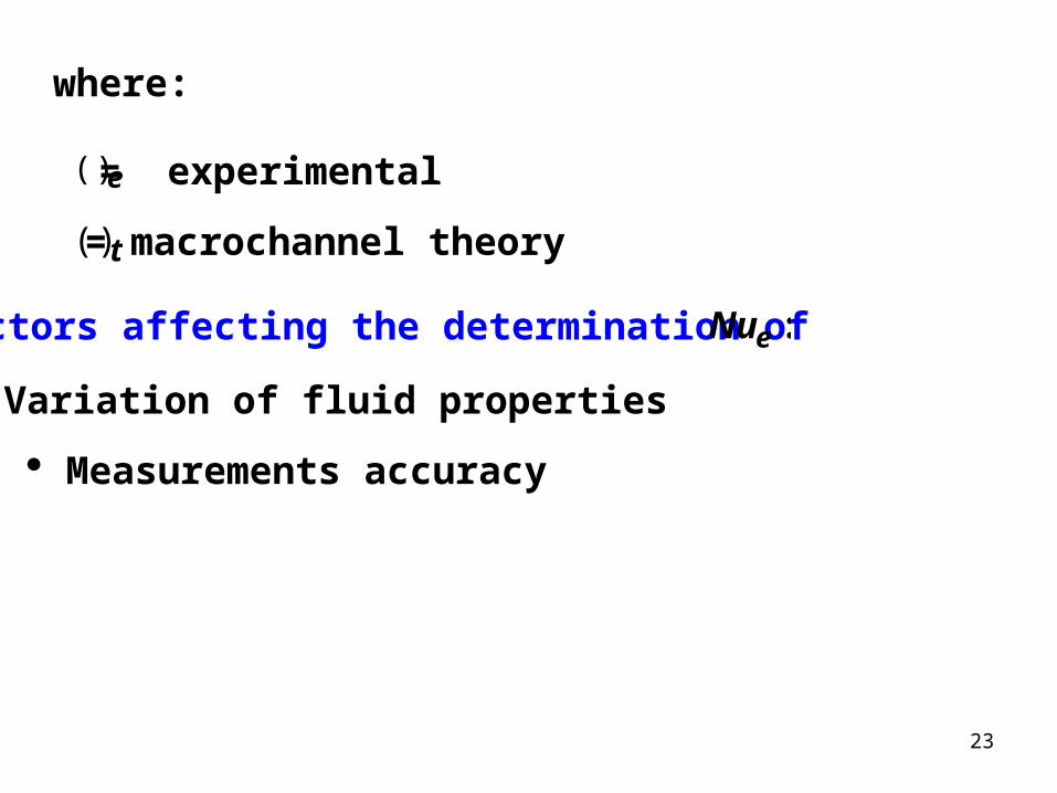
where:

e)( = experimental

t)( = macrochannel theory

Factors affecting the determination of :euN

Variation of fluid properties

Measurements accuracy

24

11.4 Governing EquationsSlip flow regime: :1.0001.0 Kn

valid are equation energy and equations, Stokes-Navier ,Continuity

conditions boundary eReformulatfail conditions jump etemperatur-no and slip velocity-No

Factors to be considered:

Compressibility

Axial conduction

Dissipation

11.4.1 Compressibility: Expressed in terms of Mach number

sound of speed

velocity fluidM =

25

Macrochannels:

Incompressible flow, M < 1

Linear pressure drop

Microchannels:

Compressible flow

Non-linear pressure drop

Decrease in Nusselt number

11.4.2 Axial Conduction

Macrochannels: neglect axial conduction for

100 rPeRPe D (6.30)

26

Pe = Peclet number

Microchannels: low Peclet numbers, axial conduction may be important, it increases the Nusselt number

11.4.3 Dissipation

Microchannels: large velocity gradient, dissipation may become important

11.5 Slip Velocity and Temperature Jump Boundary ConditionsSlip velocity for gases:

n

xuuxu

u

us

)0,(2)0,(

(11.10)

27

)0,(xu = fluid axial velocity at surface

su surface axial velocity

x = axial coordinate

n = normal coordinate measured from the surface

= tangential momentum accommodating coefficient u

Temperature jump for gases

n

xT

PrTxT

T

Ts

)0,(

1

22)0,(

(11.11)

T(x,0) = fluid temperature at the boundary

sT = surface temperature

28

vp cc / , specific heat ratio

T = energy accommodating coefficient

NOTE

(1) Eq. (11.10) and (11.11) are valid for gases

(2) Eq. (11.10) and (11.11) are valid for Kn < 0.1

(3) σu and σT, are:

• Empirical factors

• They depend on the gas, geometry and surface

• Values range from zero (perfectly smooth) to unity

29

• Difficult to determine experimentally

• Values for various gases are approximately unity

30

Examples:

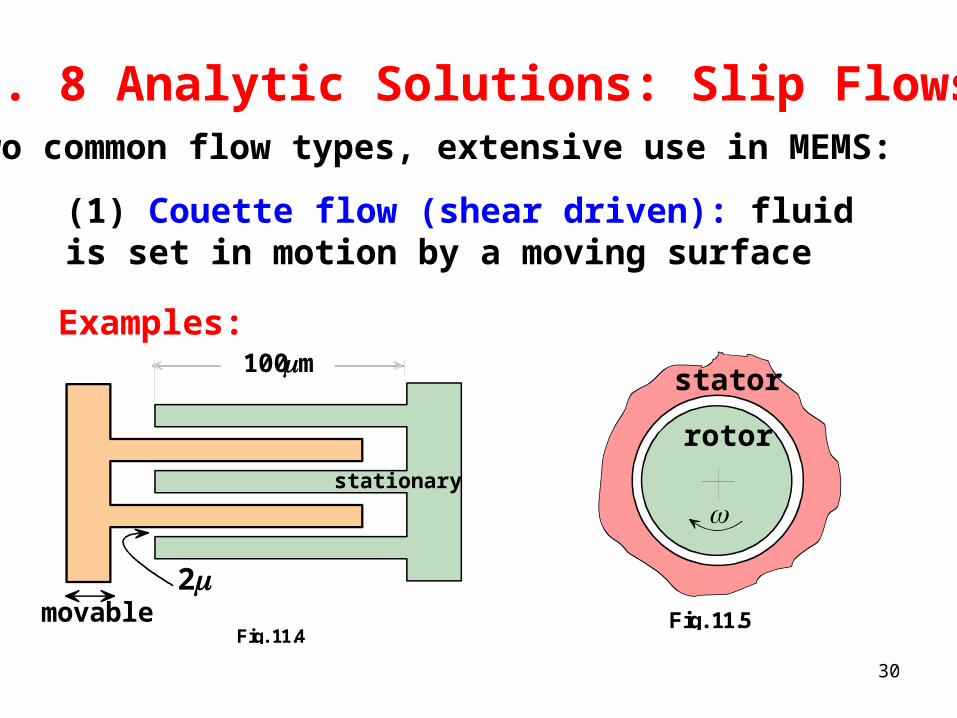
11.4. 8 Analytic Solutions: Slip Flows

Two common flow types, extensive use in MEMS:

(1) Couette flow (shear driven): fluid is set in motion by a moving surface

Fig. 11.4

2

m100

stationary

movable

Fig. 11.5

rotor

stator

31

(2) Poiseuille flow (pressure driven): fluid is set in motion by an axial pressure gradient

Examples:

Micro heat exchangers, mixers, microelectronic heat sinks

NOTE

No pressure drop in Couette flow

Signifiant pressure drop in Poiseuille flow

Boundary conditions: two types:

(1) Uniform surface temperature

(2) Uniform surface heat flux

32

11.6.1 Assumptions

(1) Steady state

(2) Laminar Flow

(3) Two-dimensional

(4) Slip flow regime (0.001 < Kn < 0.1)

(5) Ideal gas

(6) Constant viscosity, conductivity and specific heats

(7) Negligible lateral variation of density and pressure

(8) Negligible dissipation (unless otherwise stated)

(9) Negligible gravity

33

(10) The accommodation coefficients are equal to unity,

0.1 Tu

11.6.2 Couette Flow with Viscous Dissipation: Parallel Plates with Surface Convection

Gas fills gap between plates

Infinitely large parallel plates

Upper plate: moves with velocity us

Lower plate: stationary, insulated

Convection at the upper plate

Consider dissipation and slip conditions

suTy

Fig. 11.6

xHu

oh

34

Determine:

(1) Velocity distribution

(2) Mass flow rate

(3) Nusselt number

Find flow field and temperature distribution

Flow Field

Normal velocity and all axial derivatives vanish Axial component of the Navier-Stokes equations, (2.9), simplifies to

02

2

dy

ud(11.12)

35

Boundary conditions: use (11.10), Set 1u

• Lower plate: n = y = 0 and ,0su (11.10) gives

dy

xduxu

)0,()0,( (g)

Upper plate: n = H – y, (9.10) gives

dy

HxduuHxu s

),(),( (h)

Solution

)(21

1Kn

H

y

Knu

u

s

(11.14)

36

Kn is the local Knudsen number

HKn

(11.13)

NOTE

(1) Fluid velocity at the moving plate: set y = H in (11.14)

121

1)(

Kn

Kn

u

Hu

s

Effect of slip: Decrease fluid velocity at the moving plate

Increase fluid velocity at the stationary plate

37

(2) Velocity distribution is linear

(3) Setting Kn = 0 in (11.14) gives the no-slip solution

H

y

u

u

s (k)

Mass Flow Rate m

H

dyuWm0

(11.15)

W = channel width

Neglect variation of ρ along y, (11.14) into (11.15)

38

2su

WHm (11.16)

Flow rate is independent of the Knudsen number

Compare with macrochannel flow rate mo

(k) into (11.15)

2s

ou

WHm (11.17)

This is identical to (11.16), thus

1om

m(11.18)

39

Nusselt Number

• Equivalent diameter for parallel plates, De = 2H

• Nusselt number

k

HhNu

2 (l)

Heat transfer coefficient h:

sm TTy

HTk

h

)(

40

sm TTy

HT

HNu

)(

2 (11.19)

k = conductivity of fluid

T = fluid temperature

Ts = plate temperature

NOTE

(1) Fluid temperature at the moving plate, T (x,H), is not equal to surface temperature

(2) h is defined in terms of surface temperature Ts

41

(3) Use temperature jump, (11.11), to determine Ts

(4) For the upper plate, n =H – y, eq. (11.11) gives

y

HxT

PrHxTTs

),(

1

2),(

(11.20)

• Mean temperature Tm: defined in Section 6.6.2

H

pmp dyTucWTmc0

(11.21)

• Neglect variation of cp and ρ along y, use (11.14) . for u and (11.15) for m

42

H

sm dyTu

HuT

0

2(11.22)

Determine temperature distribution:

Use energy equation, (2.15) Apply above assumptions, note that axial derivatives vanish, (2.15) gives

02

2

y

Tk (11.23)

43

(2.17) gives the dissipation function which simplifies to

2

y

u (11.24)

(9.24) into (9.23)

2

2

2

dy

du

kdy

Td (11.25)

Boundary conditions

Lower plate:

0)0(

dy

dT(m)

44

Upper plate:

)()(

TThdy

HdTk so

Use (920) to eliminate Ts

T

n

HxTHxTh

dy

HdTk o

),(

1

2),(

)(

Pr

(n)

Use velocity solution (9.14), solve for T

THPr

KnH

h

kHyT

o

2

22

1

2

22(11.26)

45

where

2

)21(

KnH

u

ks (p)

Velocity solution (11.14), temperature solution (11.26) giveTs , Tm and Nu

Th

kHT

os

(u)

TH

Pr

Kn

h

kHKnHH

KnT

om

222

1

2

3

2

4

1

21

1(w)

46

Pr

KnKn

Kn

Nu

1

2

3

2

4

1

21

12

(11.27)

Note the following regarding the Nusselt number

(1) It is independent of Biot number

(2) It is independent of the Reynolds number

(3) Unlike macrochannels, it depends on the fluid

(4) First two terms in the denominator of (11.27) represent rarefaction (Knudsen number). The second term represents effect of temperature jump

47

(5) Nusselt number for macrochannels, Nuo: set Kn = 0 in (11.27):

8oNu (11.28)

Ratio of (11.27) and (11.28)

Pr

KnKn

Kn

Nu

Nu

o1

8

3

81

21

(11.29)

NOTE: Ratio is less than unity

48

11.6.3 Fully Developed Poiseuille Channel Flow: Uniform Surface Flux

Pressure driven flow between parallel plates

Fully developed velocity and temperature

Inlet and outlet pressures are pi and po

• Uniform surface flux, sq

Determine:

(1) Velocity distribution

(2) Pressure distribution

(3) Mass flow rate

(4) Nusselt number

H /2

H /2

y

x

sq

sq

Fig. 11.7

49

Note: 0x

p

Major difference between macro and micro fully developedslip flow:

Macrochannels: incompressible flow

(1) Parallel streamlines

(2) Zero lateral velocity component (v = 0)

(3) Invariant axial velocity )0/( xu

(4) Linear axial pressure constant)dxdp /(

50

Microchannels: compressibility and rarefaction change above flow pattern:

(1) None of above conditions hold

(2) Large axial pressure drop density changes compressible flow

(3) Rarefaction: pressure decreases increases Kn increases with x

(4) Axial velocity varies with axial distance

(5) Lateral velocity v does not vanish

(6) Streamlines are not parallel

(7) Pressure gradient is not constant

51

Assumptions

(1) Steady state

(2) Laminar flow

(3) 1/ RH

(4) Two-dimensional

(5) Slip flow regime (0.001 < Kn < 0.1)

(6) Ideal gas

(7) Constant viscosity, conductivity and specific heats

(8) Negligible lateral variation of density and pressure

(9) 0.1 Tu

52

(10) Negligible dissipation

Flow Field

Additional assumptions:

(11) Isothermal flow

(12) Negligible inertia forces: )(y

vv

x

uu

= 0

(13) The dominant viscous force is 2

2

y

u

Navier-Stokes equations (2.9) simplify to:

02

2

y

u

x

p (c)

53

Boundary conditions:

Symmetry at y = 0

00

y

xu ),( (e)

For the upper plate, n = H – y

y

HxuHxu

)2/,(

)2/,( (f)

Solution to u

2

22

4)(418 H

ypKn

dx

dpHu

(11.30)

54

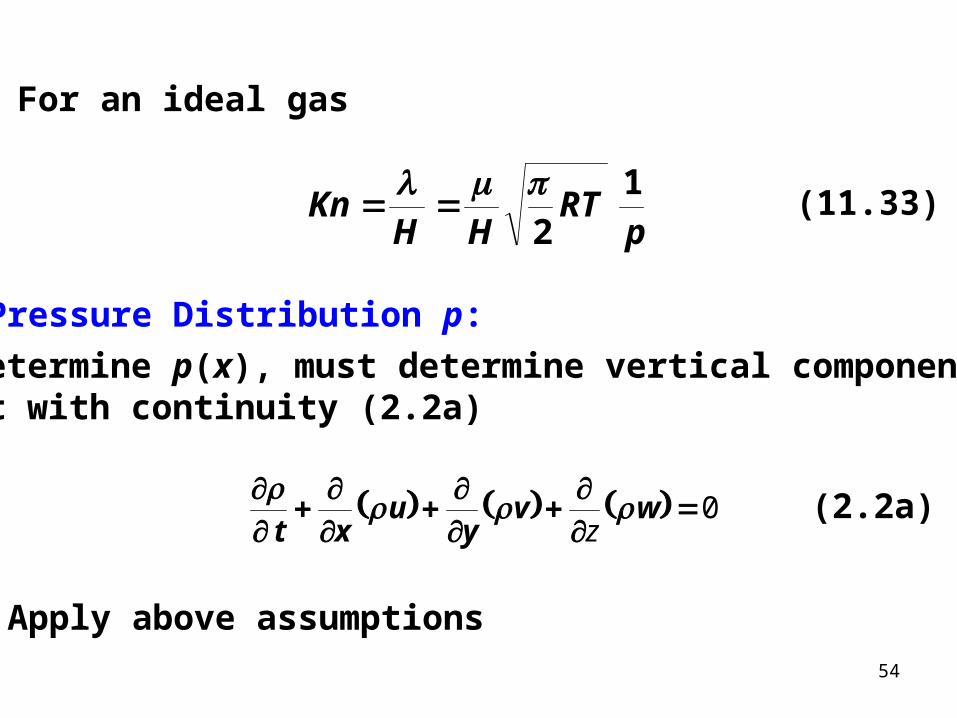
For an ideal gas

pRT

HHKn

1

2

(11.33)

Pressure Distribution p:

To determine p(x), must determine vertical component v: start with continuity (2.2a)

0

wvy

uxt

z

(2.2a)

Apply above assumptions

55

0

vy

ux

(h)

Use ideal gas to eliminate ρ:

RT

p (11.31)

(11.31) into (h), assuming constant temperature

upx

py

v (i)

(11.30) into (i)

56

)(

2

22)( 441

8 H

ypKn

dx

dpp

x

Hvp

y)(

(j)

Boundary conditions:

00 ),(xv (k)

02 )/,( Hxv (l)

Multiply (j) by dy, integrate and using (k)

dyH

ypKn

dx

dpp

x

Hvpd

yy

0 2

22

0)( 441

8)()(

(m)

57

Evaluate the integrals

3

33

3

441

1

8 H

y

H

ypKn

dx

dpp

xp

Hv )(

(11.32)

Determination of p(x): Apply boundary condition (l) to (11.32)

03

4)(41

23

3

/HyH

y

H

ypKn

dx

dpp

x(n)

Express Kn in terms of pressure. Equations (11.2) and (11.13) give

pRT

HHKn

1

2

(11.33)

58

Evaluate (n) at y = H/2, substitute (11.33) into (n) and integrate

Cp

RTHdx

dpp

12

3

1

Integrate again (T is assumed constant)

DCxpRTH

p

26

1 2 (o)

Solve for p

DCxH

RTRTH

xp 6618232

2

)( (p)

59

Pressure boundary conditions

ipp )(0 , opLp )( (q)

Apply (q) to (p)

)()( ioio ppRTHL

ppL

C 2

6

1 22

ii pRT

H

pD

26

2

Substitute into (p) and normalize by po

60

o

i

oo

i

o

i

oo

i

o

oo

p

pRT

Hpp

p

L

x

p

pRT

Hpp

p

p

RT

H

RTHpp

xp

26

126

118

23

2

22

222

2

)(

)(

(r)

Introduce outlet Knudsen number Kno using (11.2) and (11.13)

oo

oo RT

pHH

pKn

2

)( (11.34)

Substitute (11.34) into (r)

L

x

p

pKn

p

p

p

pKnKn

p

xp

o

io

o

i

o

ioo

o

)()(

)(112166

2

22

(11.35)

61

NOTE:

(1) Unlike macrochannel Poiseuille flow, pressure variation along the channel is non-linear(2) Knudsen number terms represent rarefaction effect

(3) The terms (pi/po)2 and [1- (pi/po)2](x/L) represent the effect of compressibility(4) Application of (11.35) to the limiting case of Kno =0 gives

L

x

p

p

p

p

p

xp

o

i

o

i

o)(

)(2

2

2

2

1 (11.36)

This result represents the effect of compressibility alone

62

Mass Flow Rate

2/

02

HdyuWm (s)

W = channel width

(11.30) in (s)

dx

dppKn

WHm

)(61

12

3

(t)

Density ρ :

RT

p (11.37)

63

(11.33) gives Kn(p)

RTpHH

ppKn

2

)()(

(11.33)

(11.33) and (11.37) in (t)

dx

dpRT

Hp

RT

WHm

26

12

3

(11.38)

(11.35) into (11.38) and let T=To

)( 124121

24

12

3 22

o

io

o

i

o

o

p

pKn

p

p

LRT

pHWm

(11.39)

64

Compare with no-slip, incompressible macrochannel case:

1

12

1 23

o

ioo p

p

LRT

pHWm

(11.40)

Taking the ratio

o

o

i

oKn

p

p

m

m121

2

1 (11.41)

NOTE

(1) Microchannels flow rate is very sensitive to H

(2) (11.39) shows effect of rarefaction (slip) and compressibility on m

65

(3) Since ,1/ oi pp (11.41) shows that neglecting

compressibility and rarefaction underestimates m

Nusselt Number

k

HhNu

2 (u)

For uniform surface flux sq

ms

s

TT

qh

Substitute into (g)

)(

2

ms

s

TTk

qHNu

(v)

66

Plate temperature Ts: use (11.11)

y

HxTHxTTs

)2/,(

1

2)2/,(

Pr

(11.42)

Mean temperature Tm:

2/

0

2/

0H

H

m

udy

dyTuT (11.43)

Need u(x,y) and T(x,y)

Velocity distribution: (11.30) gives u(x,y) for isothermal flow

67

Additional assumption:

(14) Isothermal axial velocity solution is applicable

(15) No dissipation, 0

(16) No axial conduction, 2222 // yTxT

(17) Negligible effect of compressibility on the energy equation

(18) Nearly parallel flow, 0v

Energy equation: equation (2.15) simplifies to

2

2

y

Tk

x

Tuc p

(11.44)

68

Boundary conditions:

0)0,(

y

xT (w)

sqy

HxTk

)2/,( (x)

To solve (11.44), assume:

(19) Fully developed temperature

Solution: T(x,y) and Tm(x): Define

)()/,(

),()/,(

xTHxT

yxTHxT

m

2

2 (11.45)

69

Fully developed temperature: is independent of x

)( y (11.46)

Thus

0

x

(11.47)

(11.45) and (11.46) give

02

2

)()/,(

),()/,(

xTHxT

yxTHxT

xx m

70

Expanding and use (11.45)

022

dx

xdT

dx

HxdTy

x

T

dx

HxdT m )()/,()(

)/,( (11.48)

Determine:

,),(

x

yxT

dx

HxdT )/,( 2and

dx

xdTm )(

Heat transfer coefficient h:

)()(

)/,(

xTxT

y

HxTk

hsm

2

(y)

71

(11.42) gives Ts(x). (11.45) gives temperature gradient in (y)

)]()/,([)/,(),( xTHxTHxTyxT m 22

Differentiate

dy

HdxTHxT

y

HxTm

)/()]()/,([

)/,( 22

2

(z)

(z) into (y), use (11.42) for Ts(x)

dy

Hd

xTxT

xTHxTkh

ms

m )/(

)()(

)]()/,([ 22

(11.49)

72

Newton’s law of cooling:

)()( xTxT

qh

ms

s

Equate with (11.49)

constant)/(

)()/,(

dy

Hdq

xTHxT sm 2

2 (11.50)

Differentiate

02

x

xT

x

HxT m )()/,(

Combine this with (11.48)

73

x

T

dx

xdT

dx

HxdT m

)()/,( 2 (11.51)

NOTE:

(11.51) replaces x

T

with dx

dTm in (11.44)

Determine dx

dTm :

Conservation of energy for element: sq

dx

dxdx

dTT m

m mT

sq

Fig. 11.8

m

74

Conservation of energy for element:

dx

dx

dTTmcTmcWdxq m

mpmps2

Simplify

p

sm

mc

qW

dx

dT

2= constant (aa)

However

muWHm (bb)

(bb) into (aa)

75

Huc

q

dx

dT

mp

sm

2

= constant (11.52)

(11.52) into (11.51)

Huc

q

x

T

dx

xdT

dx

HxdT

mp

sm

22 )()/,(

(11.53)

(11.53) into (11.44)

m

s

u

u

kH

q

y

T

22

2(11.54)

76

Mean velocity:

2

0

2 /H

m udyH

u (cc)

(11.30) gives velocity u. (11.30) into (cc)

2

0 2

22441

4

/H

m dyH

yKn

dx

dpHu

Integrate

Kndx

dpHum 61

12

2

(11.55)

77

Combining (11.30) and (11.55)

2

2

4

1

61

6

H

yKn

Knu

u

m(11.56)

(11.56) into (11.54)

2

2

2

2

4

1

61

12

H

yKn

kH

q

Kny

T s (11.57)

Integrate twice

)()()(

),( )( xgyxfH

yyKn

kHKn

qyxT s

2

4

124

1

2

1

61

12 2 (dd)

78

f(x) and g(x) are “constants” of integration

Boundary condition (w) gives

0)(xf

Solution (dd) becomes

)()(

),( )( xgH

yyKn

kHKn

qyxT s

2

4

124

1

2

1

61

12 2 (11.58)

NOTE:

(1)Boundary condition (x) is automatically satisfied

(2) g(x) is determine by formulating Tm using two methods

79

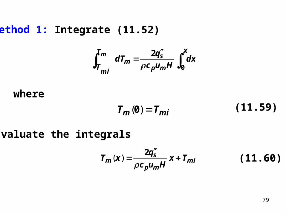
Method 1: Integrate (11.52)

x

Tdx

Huc

qdT

mp

sT

mi

mm

0

2

where

Evaluate the integrals

mim TT )(0 (11.59)

mimp

sm Tx

Huc

qxT

2

)( (11.60)

80

Method 2: Use definition of Tm. Substitute (11.30) and(11.58) into (11.43)

2

02

2

2

0 2

4

2

2

4418

124

1

2

1

61

12441

82

/

/

)( )()(

)(H

Hs

m

dyH

yKn

dx

dpH

dyxgH

yyKn

kHKn

q

H

yKn

dx

dpH

xT

Evaluate the integrals

)()()(

)( xgKnKnKnk

HqxT s

m

560

13

40

13

61

3 22

(11.61)

Equating (11.60) and (11.61) gives g(x)

560

13

40

13

61

32 22

KnKnKnk

Hqx

Huc

qTxg s

mp

smi )(

)()(

(11.62)

81

(11.58) into (11.42) gives Ts

)()(

)( xgKnPrk

HqKn

Knk

HqxT ss

s

1

2

48

5

2

1

61

3

(11.63)

The Nusselt number is given in (v)

)(

2

ms

s

TTk

qHNu

(v)

(11.61) and (11.63) into (v)

Pr

KnKnKn

KnKn

Kn

Nu

1

2

560

13

40

13

61

1

48

5

2

1

61

3

2

2

)()()(

(11.64)

82

NOTE:

(1) Kn in (11.64) depends of local pressure p

(2) Pressure varies with x, Kn varies with x

(3) Unlike macrochannels, Nu is not constant

(4) Unlike macrochannels, Nu depends on the fluid

(5) No-slip Nu for macrochannel flow, Nuo: set Kn = 0 in (11.64)

235.817

140oNu (11.65)

0

Nu

Kn0 0.04 0.08 0.124

6

8

Fig. 11.9 Nusselt number for air

83

This agrees with Table 6.2

(6) Rarefaction and compressibility decrease the Nusselt number

84

11.6.4 Fully Developed Poiseuille Channel Flow: Uniform Surface Temperature

Repeat Section 11.6.3 with plates at uniform surfacetemperature Ts

Flow field: same for both cases:

(11.30) u(y)

(11.35) opxp /)(

(11.35) m

Energy equation: (11.44) is modified to include axial conduction

H /2

H /2

y

x

sT

sTFig. 11.10

85

Boundary conditions: different for the two cases

Nusselt number:

y

HxT

TxT

H

k

HhNu

sm

)2/,(

)(

22(11.66a)

Need T(x,y) and Tm(x)

Solution approach:

Solve the Graetz channel entrance problem and setx to obtain the fully developed solution

86

Axial conduction: can be neglected for:

100PrRePe (7.50)

Microchannels:

Small Reynolds Small Peclet number Axial

conduction is important

Include axial conduction: modify energy equation (11.44)

)(2

2

2

2

y

T

x

Tk

x

Tuc p

(11.67a)

87

Boundary and inlet conditions:

0)0,(

y

xT (11.68a)

y

HxTKn

Pr

HTHxT s

)2/,(

1

2)2/,(

(11.69a)

iTyT ),0( (11.70a)

sTyT ),( (11.71a)

88

Axial velocity

2

2

4

1

61

6

H

yKn

Knu

u

m(11.56)

Solution

Use method of separation of variables

• Specialize to fully developed: set x

Result: Fig. 11.11 shows Nu vs. Kn

Nu

Kn0 0.04 0.08 0.12

5

6

7 8

8

Fig. 11.11 Nusselt number for flow between parallel plates at uniform surface temperature for air, Pr = 0.7,

4.1 , 1 Tu , [14]

Pe = 015

89

NOTE

(1) Nu decreases as the Kn is increased

(2) No-slip solution overestimates microchannels Nu

(3) Axial conduction increases Nu

(4) Limiting case: no-slip (Kn = 0) and no axial conduction

)( Pe : 5407.7oNu (11.73)

This agrees with Table 6.2

Heat Transfer Rate, sq :

Following Section 6.5

90

])([ mimps TxTcmq (6.14)

Tm (x) is given by

][exp)()( xcmhP

TTTxTp

smism (6.13)

,h is determine numerically using (6.12)

x

dxxhx

h0

)(1

(6.12)

91

11.6.5 Fully Developed Poiseuille Flow in Micro Tubes: Uniform Surface Flux

Consider:

Poiseuille flow in micro tube

Uniform surface flux

Fully developed velocity and temperature

• Inlet and outlet pressures are pi and po

sq

sq

Fig. 11.12

z

orr r

92

Determine

(1) Velocity distribution

(2) Nusselt number

Rarefaction and compressibility affect flow and heat transfer Velocity slip and temperature jump

Axial velocity variation

Lateral velocity component

Non-parallel stream lines

Non-linear pressure

93

Assumptions

Apply the 19 assumptions of Poiseuille flow between parallel plates (Sections 11.6.3)

Flow Field

Follow analysis of Section 11.6.3 Axial component of Navier-Stokes equations in cylindrical coordinates:

z

p

r

vr

rrz

11

)( (a)

),( zrv z = axial velocity

94

Boundary conditions:

Assume symmetry and set σu = 1

0),0(

r

zv z (b)

r

zrvzru oz

o

),(

),( (c)

Solution

2

2241

4 o

oz

r

rKn

dz

dprv

(11.74)

95

Knudsen number

orKn

2

(11.75)

Mean velocity vzm

or

drvrr

v zo

zm02

21

Use (11.74), integrate

)81(8

2Kn

dz

dprv o

zm

(11.76)

96

(11.74) and (11.76)

Kn

rrKn

v

v o

zm

z

81

)/(412

2

(11.77)

Solution to axial pressure

L

z

p

pKn

p

p

p

pKnKn

p

zp

o

io

o

i

o

ioo

o

)1(16)1(88

)(2

22

(11.78)

(11.76) and (11.78) give m

)( 1161

16 2

224

o

io

o

ioo

p

pKn

p

p

LRT

prm

(11.79a)

97

For incompressible no-slip (macroscopic)

)( 18

24

o

iooo p

p

LRT

prm

(11.79b)

Nusselt Number

Follow Section 11.6.3

k

hrNu o2

(d)

Heat transfer coefficient h:

ms

s

TT

qh

98

Substituting into (d)

)(

2

ms

so

TTk

qrNu

(e)

Ts = tube surface temperature, obtained from temperaturejump condition (11.11)

r

zrT

PrzrTT o

os

),(

1

2),(

(f)

Mean temperature:

o

o

rrdrv

rdrrTv

T

z

z

m

0

0 (11.80)

99

Energy equation:

)(r

Tr

rr

k

z

Tvc zp

(11.81)

Boundary conditions:

00

r

zT ),( (g)

so qr

zrTk

),(

(h)

Define

100

)(),(

),(),(

zTzrT

zrTzrT

mo

o

(11.82)

Fully developed temperature:

)(r (11.83)

Thus

0

z

(11.84)

(11.82) and (11.84) give

0

)(),(

),(),(

zTzrT

zrTzrT

zz mo

o

101

Expand (11.82)

0

zd

zdT

zd

zrdTr

z

T

zd

zrdT moo )(),()(

),( (11.85)

Determine:

,),(

z

zrT

dz

zrdT o ),( and dz

zdTm )(

Heat transfer coefficient h,:

)()(

),(

zTzT

r

zrTk

hsm

o

(i)

102

Rewrite (11.81)

)](),([),(),( zTzrTzrTzrT moo

Differentiate and evaluating at orr

dr

rdzTzrT

r

zrT omo

o )()](),([

),(

(j)

(j) into (i)

dr

rd

zTzT

zTzrTkh o

ms

mo )(

)()(

)](),([

(k)

103

Newton’s law of cooling h

)()( zTzT

qh

ms

s

Equate with (k)

constant)(

)(),(

dr

rdk

qzTzrT

o

smo (11.86)

Differentiate

0

z

zT

z

zrT mo )(),(

104

Combine with (11.85)

z

T

zd

zdT

zd

zrdT mo

)(),( (11.87)

Will use (11.87) to replace zT / in (11.81) with ./ dzdTm

Conservation of energy to dx

dz

dz

dTTmcTmcdzqr m

mpmpso2 sq

dx

dxdx

dTT m

m mT

sq

Fig. 11.13

m

105

Simplify

p

som

mc

qr

dz

dT

2 (l)

However

mzovrm 2 (m)

(m) into (l)

mzop

sm

vrc

q

dz

dT

2

(11.88)

(11.88) into (11.87)

mzop

smo

vrc

q

z

T

zd

zdT

zd

zrdT

2)(),(

(11.89)

106

(11.89) into (11.81)

rv

v

kr

q

r

Tr

r mz

z

o

s

2)( (11.90)

(11.77) is used to eliminate mzz zv / in the above

rr

rKn

kr

q

Knr

Tr

r oo

s

2

241

81

4)( (11.91)

Integrate

)()()()(

),( zgyzfr

rrKn

rkKn

qzrT

oo

s

2

42

4

141

81(n)

107

Condition (g) gives

0)(zf

Solution (n) becomes

)()(

),( )( zgr

rrKn

rkKn

qzrT

oo

s

2

42

4

141

81(11.92)

Condition (h) is automatically satisfied

Determine g(z): Use two methods to determine Tm

Method 1: Integrate (11.88)

108

zdz

rvc

qdT

omzp

sT

Tm

m

mi0

2

where mim TT )(0 (11.93)

Evaluate the integral

miomzp

sm Tz

rvc

qT

2

(11.94)

Method 2: Use definition of Tm in (11.80). Substitute (11.74)and (11.92) into (11.80)

109

o

o

r

r

rdrr

rKn

drrzgr

rKn

krKn

q

r

rKn

T

o

o

ro

s

om

02

2

0 2

42

2

2

41

164

1

81

441 )(

)()(

Integrate

)()(

zgKnKnKnk

rqT os

m

24

7

3

1416

812

2 (11.95)

Equate (11.94) and (11.95), solve for g(z)

24

7

3

1416

81

2 22

KnKnKnk

rqz

vrc

qTzg os

mzop

smi

)()(

(11.96)

110

Use (f) and (11.92) to determine ),( zrT os

)()(

),( zgKnPrk

rqKn

Knk

rqzrT osos

os

1

4

16

3

81

4

(11.97)

Nusselt number: (11.95) and (11.97) into (e)

KnKnKnKn

KnKn

Nu

Pr

1

)()()(

1

4

24

7

3

1416

81

1

16

3

81

42

2

2

(11.98)

111

Results: Fig. 11.14

Fig. 11.14 gives Nu vs. Kn for air

• Rarefaction and compressibility decrease the Nusselt number Nusselt number depends on the fluid

• Nu varies with distance along channel

• No-slip Nusselt number, Nuo, is obtained by setting Kn = 0 in (11.97)

364.411

48oNu (11.99)

Nu

Kn0 0.04 0.08 0.122.0

3.0

4.0

Fig. 11.14 Nusselt number for air flow through tubes at unifrorm surface heat flux

112

This agrees with (6.55) for macro tubes

11.9.6 Fully Developed Poiseuille Flow in Micro Tubes: Uniform Surface Temperature• Repeat Section 11.6.5 with the tube at surface temperature Ts

Apply same assumptions

Boundary conditions are different

Flow field solution is identical for the two cases

Fig. 11.15

z

orr r

sT

113

Nusselt number:

r

zrT

TzT

r

k

hrNu o

sm

oo

),(

)(

22(11.100a)

• Determine T(r,z) and Tm(z)

Follow the analysis of Section 11.6.4

Solution is based on the limiting case of Graetz tube entrance problem

Axial conduction is taken into consideration

Energy equation (11.81) is modified to include axial conduction:

114

2

2)(

z

Tk

r

Tr

rr

k

z

Tvc zp

(11.101a)

Boundary and inlet conditions

0)0,(

z

rT (11.102a)

r

zrTKn

Pr

rTzrT oo

so

),(2

1

2),(

(11.103a)

iTrT )0,( (11.104a)

sTrT ),( (11.105a)

115

(11.76) gives axial velocity

Kn

rrKn

v

v o

zm

z

81

)/(412

2

(11.76)

Solution by the method of separation of variables

Solution is specialized for fully developed conditions at large z

• Result for air shown in Fig. 11.16

Neglecting axial conduction: set Pe

Axial conduction increases the Nu

116

• Limiting case: no slip and no axial conduction: at Kn = 0 and Pe

657.3oNu (11.72)

This agrees with (6.59)

• Limiting case: no slip with axial conduction: at Kn =0 and Pe = 0:

1754.oNu

N u

K n

2.5

2 .0

3 .0

3 .5

4 .0

4 .5

0 0 .0 4 0 .0 8 0 .1 2

F ig . 1 1 .1 6 N u sselt n u m b er for flow th rou gh tu b es a t u n iform su rface tem p eratu re for a ir