ME597/Math597/Phy597Spring 2019

1 Introduction to Information and Entropy

Let X be a random variable with (discrete) finitely many outcomes; let us call these outcomes as symbols,x1, · · · , xM, where M ≥ 2. Examples are as follows:

1. A coin, identified by two symbols as Head and Tail, is flipped many times and each flip is an independentBernoulli trial. Here, the symbol alphabet Σ= Head, Tail and the alphabet size |Σ| = 2.

2. A six-faced die, identified by six symbols as 1, 2, 3, 4, 5, and 6, is rolled many times and each roll isan independent trial. Here, Σ = 1, 2, 3, 4, 5, 6 and |Σ| = 6.

3. An ideal gas system, contained in a rigid, impermeable, and diathermal vessel, consists of a very largenumber (N) of non-interacting molecules. Under (quasi-static) thermodynamic equilibrium conditions,the system may have M energy states (denoted as symbols and |Σ| =M), where 2 ≤M ≪ N .

Let the random variable X have a probability distribution, described by a probability mass function pi,where

∑Mi=1 pi = 1 and pi ≥ 0 ∀i. Now, we pose the following question:

What is the information content of X (i.e., the expected value of log of the probability massfunction pi : i = 1, 2, · · · ,M)?

To answer the above question, let us construct a finite-length (N -long) string (e.g., word) of symbols, whichis constructed from N independent realizations of the random variable X, where N ≫ M . Let us find outhow many binary digits (called bits) are needed to construct this N -long string. If there are R bits, then itfollows that (

2R =MN

)⇒

(R log 2 = N logM

)⇒

(R =

N logM

log 2

)Taking the the logarithm with base 2, it follows that R = N log2M . Apparently, an N -long string ofindependent trials of the random variable X has an information content of N log2M bits, i.e., this many bitsof information will have to be generated to construct the string.

The probability distribution pi limits the types of strings that are likely to occur. For example, if pj ≫ pk,then it is very unlikely to construct a string with the number of xk’s being larger than the number of xj ’s.

For N → ∞, we expect that xj will appear approximately (nj , Npj) times out of N . Therefore, a typical

string will contain ni , Npi; i = 1, · · · ,M symbols arranged in different ways. The number of differentarrangements is given by

η(N,M) , N !

n1! · · ·nM !where

M∑i=1

ni = N and ni ≥ 0 ∀i

It is noted that η ≤ MN which is the maximum possible number of N -long strings, made of M differentsymbols. Then, it follows by using Stirling formula (which states loge k! = k loge k − k +O(loge k)) that

loge η = logeN !−M∑j=1

loge nj ! ≈(N logeN −N

)−

M∑j=1

(nj loge nj − nj

)= N logeN −

M∑j=1

nj loge nj = N logeN −M∑j=1

(Npj

)loge(Npj)

= N logeN −(N logeN

)( M∑j=1

pj

)−N

M∑j=1

pj loge pj

= −NM∑j=1

pj loge pj

1

Then, to represent one of the ”likely” η strings, it takes log2 η ≈ −N∑M

j=1 pj log2 pj bits of information.

Shannon’s Theorem states that, as N → ∞, the minimum number of bits necessary to ensure the errorsto vanish in N trials is log2 η ≈ −N

∑Mj=1 pj log2 pj , which is less than N log2M bits as needed in the

absence of any knowledge of the probability distribution pi. The difference per trial can be attributed as

the information content I of the probability distribution pi, i.e.,N log2 M+N

∑Mj=1 pj log2 pj

N , from which itfollows that

I[pi] , log2M +M∑j=1

pj log2 pj

We define the entropy of a probability distribution pi as:

H[pi] , −M∑j=1

pj log pj

Example 1.1. Let X be a (continuous) random variable whose probability density function (pdf) f(•) isunknown, but the expected value E[X] = µ and the variance V ar[X] = σ2 are computed from the physical

measurements. Find the best estimate f(•) of the unknown f(•) by maximizing the entropy:

H(X) , −∫Rlog

(f(x)

)f(x) dx

We have the following constraints on f(x):∫Rf(x)dx = 1,∫

Rxf(x)dx = µ,∫

Rx2f(x)dx = µ2 + σ2.

Define the Lagrangian:

L(x, λ) = −∫Rlog(f(x))f(x)dx+ λ0

(∫Rf(x)dx− 1

)+ λ1

(∫Rxf(x)dx− µ

)+ λ2

(∫Rx2f(x)dx− µ2 − σ2

).

The entropy attains the maximum when the following functional derivatives are equal to zero:

δL

δf(x)= −1− log(f(x)) + λ0 + λ1x+ λ2x

2 = 0 ∀x ∈ R, (1)

∂L

∂λ0=

∫Rf(x)dx− 1 = 0, (2)

∂L

∂λ1=

∫Rxf(x)dx− µ = 0, (3)

∂L

∂λ2=

∫Rx2f(x)dx− µ2 − σ2 = 0. (4)

By (1) we can obtain

f(x) = e−1+λ0+λ1x+λ2x2

∀x ∈ R. (5)

Substituting (5) into (2), (3) and (4), by using the technique of integration by parts, we can obtain that

λ0 = 1− µ2

2σ2− log(σ

√2π), λ1 =

µ

σ2, λ2 = − 1

2σ2. (6)

Substituting (6) into (5), we have

f(x) =1

σ√2πe−

(x−µ)2

2σ2 . (7)

2

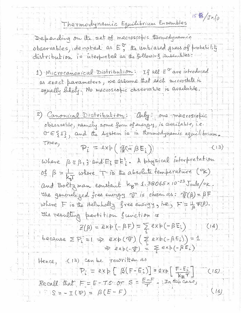
2 A Thermodynamic Perspective

Let a vessel with rigid, impermeable, and diathermal boundaries contain N (non-interacting and statisticallyindependent) randomly moving particles. Under a thermodynamic equilibrium condition, let the total energyof these N particles be E that is distributed as follows:

Let N particles be clustered in M groups, where M ≥ 2 and M ≪ N . In group i, where i = 1, 2, · · · ,M ,there are ni particles such that the expected value of the energy of each particle is εi with standard deviationδi. Let us order these M groups of particles such that ε1 < ε2 < · · · < εM . It is assumed that

(δiεi

)≪ 1

and(√

δ2i+δ2i+1

εi+1−εi

)≪ 1. Let us define pi , ni

N and Ei , Nεi, where i = 1, 2, · · · ,M ; obviously,∑M

i=1 pi = 1

and E1 < E2 < · · · < EM and E =∑M

i=1(piEi). It follows from the principle of energy minimization at anequilibrium condition that p1 > · · · > pM . Then,

N =

M∑i=1

ni and E =

M∑i=1

niεi =

M∑i=1

(niN

) (Nεi

)=

M∑i=1

(piEi) for a very large N

Let us initiate a quasi-static change through exchange of energy via the diathermal boundaries so thatthe total energy of the thermodynamic system is now E while the number of particles is still the same.Then these N particles have a new probability distribution pi, i = 1, 2, · · · ,M because the N particles arenow distributed among the same groups as ni, i = 1, 2, · · · ,M . The following conditions hold at this newcondition.

M∑i=1

pi = 1 and E =

M∑i=1

(piEi)

Note that Ei’s are unchanged and the expected value of the energy of each of the ni particles in the ith

group is still εi for i = 1, 2, · · · ,M .

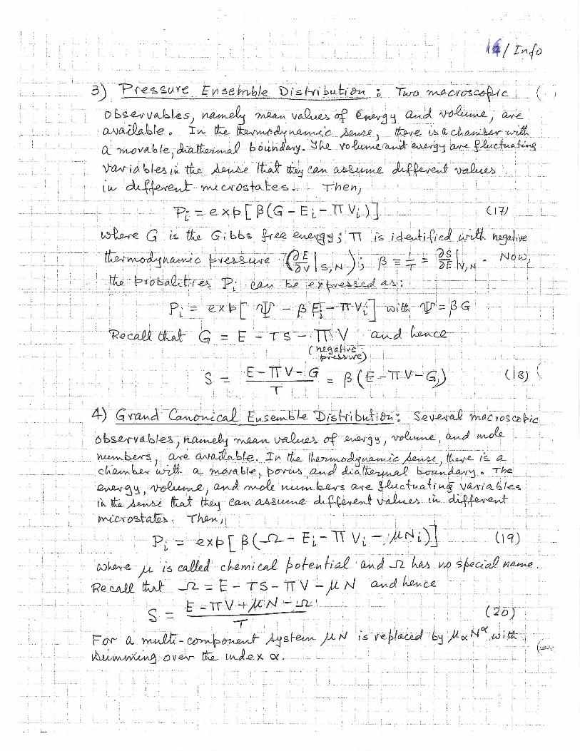
Remark 2.1. The particle energies εi are discrete according to quantum mechanics and their values dependon the volume to which these particles are confined; therefore, the possible values of the total energy E arealso discrete. However, for a large volume and consequently a large number of particles, the spacings of thedifferent energy values are so small in comparison to the total energy of the system that the parameter Ecan be regarded as a continuous variable. Note that this fact prevails regardless of whether the particles arenon-interacting or interacting.

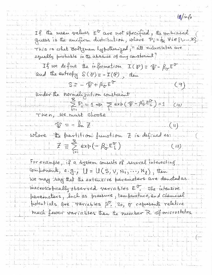
Remark 2.2. For a general case, where the vessel boundaries are allowed to be flexible, porus, and diather-mal, the specifications of the respective parameters V , N and E define a macrostate of the thermodynamicsystem. However, at the particle level, there is a very large number of ways in which a macrostate (N,V,E)can be realized. As seen above in the case of non-interacting particles, the total energy is simply the sumof the energies of N particles; since these N particles can be arranged in many different ways, each singleparticle of energy εi can be placed in many different ways to realize the total energy E. Each of these differentways specifies a microstate of the system and the actual number Ω of these microstates is a function of V ,N and E. In general, the microstates of a given system are generated in quantum mechanics as the indepen-dent solutions as wave functions ψ(r1, · · · , rN ) of the Schrodinger equation corresponding to the eigenvalueE of the relevant operator. In essence, a given macrostate of the system corresponds to a large number ofmicrostates. In the absence of any constraints, these microstates are equally probable, i.e., the system isequally likely to be in any one of these microstates at an instant of time.

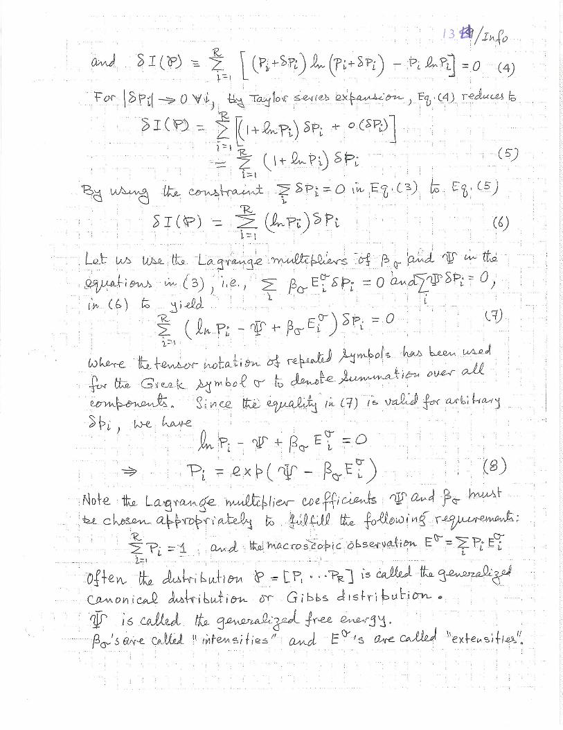
3 Information Theory

Information is viewed as a ameasure of knowledge derived from observed data if the probability distribution(and nothing else) of the data are available.

Definition 3.1. Let A be a (nonempty and finite) alphabet of symbols such that |A| ≥ 2. Let ℓ be the lengthof a word (i.e., a string of ℓ symbols) serving as a pattern. Then, the number of such patterns N ≤ |A|ℓ

3

Definition 3.2. Shannon information of a word (i.e., symbol string) of length ℓ on the alphabet A is definedas:

I(p) , log(|A|) + E[log(p)] = log(|A|) +|A|∑i=1

pi log(pi)

where p = [p1 · · · p|A|] with pi ≥ 0 and∑|A|

i=1 pi = 1.

Remark 3.1. Shannon entropy S(p) , −∑|A|

i=1 pi log(pi) is perhaps borrowed from the discipline of equilib-rium thermodynamics, where the symbol alphabet A is equivalent to collection of a finite number of energystates Ei and pi is the probability of a ith energy state being occupied by a particle under macroscopic equi-librium.

Remark 3.2. If pj = 1 and consequently pi = 0 ∀i = j, then S(p) = 0. on the other hand, p is uniformlydistributed, i.e., pi =

1|A| ∀ i, then S(p) = log |A|.

3.1 Khinchin Axioms

Khinchin (1957) introduced the following axioms:

• Axiom 1: I(p) = I(p1, · · · , p|A|) only depends on p = [p1, · · · , p|A|] and nothing else.

• Axiom 2: I(

1|A| , · · · ,

1|A| ) ≤ I

(p1, · · · , p|A|

), i.e., S

(1

|A| , · · · ,1

|A|

)≥ S

(p1, · · · , p|A|

).

• Axiom 3: I(p1, · · · , p|A|) = I(p1, · · · , p|A|, 0), which implies that augmentation of a data set withnew symbols, whose probability of occurrence is 0, does not change the information.

• Axiom 4: Let the composition of the original system Θsys with an added system Θ yield the augmentedsystem Θaug. Then,

I(paug) = I(psys) +∑i

psysi I(p|i)

where I(p|i) ,∑

j pj|i log(pj|i) is the conditional probability distribution of the added system Θ. Notethat pj|i is the probability of event j of the added system when event i of the system Θsys has occurred.

4