Computers and Chemical Engineering 32 (2008) 1943–1955
Two-phase mass transfer coefficient prediction in stirredvessel with a CFD model
F. Kerdouss, A. Bannari, P. Proulx ∗, R. Bannari, M. Skrga, Y. LabrecqueDepartment of Chemical Engineering, Universite de Sherbrooke, Sherbrooke, QC J1K 2R1, Canada
Received 23 February 2006; received in revised form 2 October 2007; accepted 17 October 2007Available online 26 October 2007
bstract
In the present paper, gas dispersion in a laboratory scale (5 L) stirred bioreactor is modelled using a commercial computational fluid dynamicsCFD) code FLUENT 6.2 (Fluent Inc., USA). A population balance model (PBE) is implemented in order to account for the combined effect ofubble breakup and coalescence in the tank. The impeller is explicitly described in three dimensions using the two-phase and Multiple Referencerame (MRF) Model. Dispersed gas and bubbles dynamics in the turbulent flow are modelled using an Eulerian–Eulerian approach with dispersed–ε turbulent model and modified standard drag coefficient for the momentum exchange. Parallel computing is used to make efficient use of the
omputational power in order to predict spatial distribution of gas hold-up, Sauter mean bubble diameter, gas–liquid mass transfer coefficient andow structure. The numerical results from different distribution of classes are compared with experimental data and good agreement is achieved.2007 Elsevier Ltd. All rights reserved.
eywords: Bioreactor; Bubble size; Computational fluid dynamics (CFD); Gas dispersion; Mass transfer; Mixing; Multiphase flow; Parallel computing; Populationalances; Stirred tank
Amatul&R1mb(KHb
. Introduction
Modelling of the complex flow in a chemical or bioprocessingeactor, in the presence of a rotating impeller, is a computa-ional challenge. Although computational fluid dynamics (CFD)ommercial codes have made impressive steps towards the solu-ion of such engineering problems over the last decade, it stillemains a difficult task to use such codes to help the designnd the analysis of bioreactors. The scientific and technical lit-rature on the subject has rapidly evolved from single-phase,otating impeller systems (Jenne & Reuss, 1997; Luo, Issa, &osman, 1994; Micale, Brucato, & Grisafi, 1999; Rutherford,ee, Mahmoudi, & Yianneskis, 1996; Tabor, Gosman, & Issa,996) to population balance methods aiming at the predictionf the disperse phase bubble sizes using different approaches
Bakker & Van Den Akker, 1994; Kerdouss, Bannari, & Proulx,006; Kerdouss, Kiss, Proulx, Bilodeau, & Dupuis, 2005; Lane,chwarz, & Evans, 2005, 2002; Venneker, Derksen, & Van Den
kker, 2002). As a function of the type of results expected,odelling of bioreactors can be made simpler to target over-
ll parametric study or more complex to try to describe finelyhe bubble size distribution. Single bubble size models can besed to decrease the computational effort while maintaining aocal description of the two-phase flow details (Deen, Solberg,
Hjertager, 2002; Friberg, 1998; Hjertager, 1998; Khopkar,ammohan, Ranade, & Dudukovic, 2005; Morud & Hjertager,996; Ranade, 1997; Ranade & Deshpande, 1999). Detailedodels using multiple bubble sizes typically more than 10 size
ins, give more information on the secondary phase behaviorAlopaeus, Koskinen, & Keskinen, 1999; Alopaeus, Koskinen,eskinen, & Majander, 2002; Dhanasekharan, Sanyal, Jain &aidari, 2005; Venneker et al., 2002). The formulation of theubble size bins equations involves transport by convectionnd source/sink terms for the coalescence or breakup (Chen,udukovic, & Sanyal, 2005a, 2005b; Sanyal, Marchisio, Fox,Dhanasekharan, 2005). Modern numerical techniques making
fficient use of the computational efficiency of modern comput-rs have to be used in order to address this problem. Slidingeshes (SM) or Multiple Reference Frames (MRF) are tech-
iques available to model the rotation of the impeller in the
1944 F. Kerdouss et al. / Computers and Chemical Engineering 32 (2008) 1943–1955
Nomenclature
a interfacial area (m−1)a(v, v
′) break frequency (s−1)
B birth (m−3 s−1)b(v) breakup frequency (s−1)C death (m−3 s−1)C∗ liquid phase dissolved oxygen saturation concen-
tartion (kg m−3)CL dissolved oxygen concentration in liquid phase
(kg m−3)CD drag coefficientc constant (1.0)cf increase coefficient of surface areaD impeller diameter (m)DO2 oxygen diffusion coefficient (m2 s−1)d bubble diameter (m)do sparger orifice (m)d32 Sauter mean diameter (m)�F volumetric force (N m−3)f fraction�g acceleration due to gravity (9.81 m s−2)H liquid height (m)¯I unit tensorH Henry’s constant (Pa kg−1 m3)K exchange coefficient (kg m−3 s−1)k1 constant (0.923)kL mass transfer coefficient (m s−1)m(v) mean number of daughter produced by breakup
(2)�N angular velocity (rad s−1)n number density of bubble class (m−3)PC coalescence efficiencyPO2 partial pressure of oxygen (Pa)p pressure (N m−2)p(v, v
′) probability
Re Reynolds number�R interphase force (N m−3)�r position vector (m)T tank diameter (m)t time (s)�U average velocity (m s−1)uij bubble approaching turbulent velocity (m s−1)u bubble turbulent velocity (m s−1)v bubble volume (m−3)We Weber numberx abscissa or pivot of the i th parent class (m3)
ε turbulent dissipation energy (m2 s−3)λ eddy size (m)μ viscosity (kg m−1 s−1)π defined in Eq. (32)θ test functionθij collision frequency (m−3 s−1)ρ density (kg m−3)σ surface tension (N m−1)τ characteristic time (s)¯τ stress tensor (kg m−1 s−2)ΩB breakup rate (m−3 s−1)ξ size ratio (λ/di)ξij size ratio (di/dj)
SubscriptsB breakupC coalescenceeff effectiveG gas phasei phase number; axis indices of space coordinates,
class indexj axis indices of space coordinates, class indexlam laminarL liquid phaset turbulent
rtooocE
2
wempoaT6otoTalf
eactor (Luo et al., 1994). Parallel computing, adaptive unstruc-ured meshes are some of the tools used to make efficient usef the computational power. In the present study we compareverall two-phase mass transfer coefficients measured in a lab-ratory scale (3 L) New Brunswick BioFlo 110 bioreactor toomputational results obtained with the CFD software FLU-NT.
. Experimental setup
A 3 L New Brunswick BioFlo 110 bioreactor (T = 12.5 cm)ith 2 L working volume is used in this study. This reactor is
quipped with automatic feedback controllers for temperature,ixing and dissolved oxygen. The mixing is driven by a 45
itched blade impeller with 3 blades (D = 0.075 cm) mountedn a 10 mm diameter shaft placed at the centerline of the biore-ctor and located at 76 mm from the headplate of the vessel.he gas is supplied through a 0.04 m diameter ring sparger withholes of 1 mm in diameter located 50 mm under the center
f the impeller (see Fig. 2). The dissolved oxygen concen-ration is measured with a polarographic-membrane dissolvedxygen probe (InPro 6800 series O2 sensors from METTLER
OLEDO) and monitored with a computer interface. The biore-ctor is de-aerated by sparging with N2 until only minimumevels of dissolved oxygen remained. At this point, air is dif-used into the reactor until saturation is achieved. In the present
emica
ptw1s3μ
0sac(
3
3
tasmbtdTa
wmLtt
α
Ta
tsr
F
g
3
ottmavbiit
R
K
K
da
R
Fo
C
Hitavd
R
CoAA0
3
ca
F. Kerdouss et al. / Computers and Ch
aper, numerical simulations are compared to the experimen-al data (conducted at 20 ◦C) of a stirred tank filled with tapater with a total height of H = 4/3T , gas flow rate of 1.0 ×0−5 m3 s−1 and an impeller rotation speed of 600 rpm corre-ponding to a turbulent Reynolds number, Re = ρLND2/μL �.75 × 104. The water properties are set as ρL = 998.2 kg m−3,L = 0.001 kg m−1 s−1. The surface tension, σ, is assumed as.073 N m−1 (CRC Handbook, 2002). The properties of air areet as ρG = 1.225 kg m−3, μG = 1.789 10−5 kg m−1 s−1. Thessumption of constant density is taken here as the pressurehange from the bottom to the surface of the vessel is lowPsurfae/Pbottom � 0.98).
. Numerical model
.1. Governing flow equations
The gas and liquid are described as interpenetrating con-inua and equations for conservation of mass and momentumre solved for each phase. The flow model is based onolving Navier–Stokes equations for the Eulerian–Eulerianultiphase model along with dispersed multiphase k–ε tur-
ulent model. FLUENT uses phase-weighted averaging forurbulent multiphase flow, and then no additional turbulentispersion term is introduced into the continuity equation.he mass conservation equation for each phase is writtens:
∂
∂t(ρiαi) + ∇ · (αiρi
�Ui) = 0.0 (1)
here ρi, αi and �Ui represent the density, volume fraction andean velocity, respectively, of phase i (L or G). The liquid phaseand the gas phase G are assumed to share space in proportion
o their volume such that their volume fractions sums to unity inhe cells domain:
L + αG = 1.0 (2)
he momentum conservation equation for the phase i after aver-ging is written as:
∂
∂t(ρiαi
�Ui) + ∇ · (αiρi�Ui
�Ui)
= −αi∇p + ∇ · ¯τeffi + �Ri + �Fi + αiρi�g (3)
p is the pressure shared by the two phases and �Ri represents
he interphase momentum exchange terms. The term �Fi repre-ents the Coriolis and centrifugal forces applied in the rotatingeference frame for the MRF model and is written as:
�i = −2αiρi
�N × �Ui − αiρi�N × ( �N × �r) (4)
The Reynolds stress tensor ¯τeffi is related to the mean velocityradients using Boussinesq hypothesis:
¯τeffi = αi(μlam,i + μt,i)(∇ �Ui + ∇ �UTi )
− 23αi(ρiki + (μlam, i + μt,it)∇ · �Ui)¯I (5)
t
μ
l Engineering 32 (2008) 1943–1955 1945
.2. Interfacial momentum exchange
The most important interphase force is the drag force actingn the bubbles resulting from the mean relative velocity betweenhe two phases and an additional contribution resulting fromurbulent fluctuations in the volume fraction due to averaging of
omentum equations (FLUENT 6.2, 2005). Other forces suchs lift and added mass force may also be significant under theelocity gradient of the surrounding liquid and acceleration ofubbles respectively. These forces and the turbulent fluctuationn the volume fraction in the drag force have not been includedn this paper. �Ri is reduced only to the drag force proportionalo the mean velocity difference, given by the following form:
�L = −�RG = K( �UG − �UL) (6)
is the liquid–gas exchange coefficient written as:
= 3
4ρLαLαG
CD
d| �UG − �UL| (7)
is the bubble diameter and CD is the drag coefficient defineds function of the relative Reynolds number Rep:
ep = ρL| �UG − �UL|dμL
(8)
or calculation of the drag coefficient, the standard correlationf Schiller and Naumann is used (Ishii & Zuber, 1979):
D =
⎧⎪⎨⎪⎩
24(1 + 0.15Re0.687p )
Rep, Rep ≤ 1000.0
0.44, Rep > 1000.0
(9)
owever, this basic drag correlation applies to bubbles movingn a still liquid and does not as such apply to bubbles moving inurbulent liquid. In this work, a modified drag law that takes intoccount the effect of turbulence is used. It is based on a modifiediscosity term in the relative Reynolds number (Bakker & Vanen Akker, 1994):
ep = ρL| �UG − �UL|dμL + Cμt,L
(10)
is the model parameter introduced to account for the effectf the turbulence in reducing slip velocity (Bakker & Van Denkker, 1994; Kerdouss et al. 2006; Laakkonen, Alopaeus, &ittamassa, 2006; Lane et al., 2002). This parameter is set to.3 (Kerdouss et al., 2006).
.3. Turbulence model equations
As the secondary phase is dilute and the primary phase islearly continuous, the dispersed k–ε turbulence model is usednd solves the standard k–ε equations for the primary phase. The
urbulent liquid viscosity μt,L in Eq. (5) is written as:
t,L = ρLCμ
k2L
εL(11)
1 emica
af
G
acRt1pgt
3
saultelfitnla(RoMQ2BmTcHa
wbatLAeos
B
D
B
D
Harepb
v
n
v∑
Et
f
w∑
(
946 F. Kerdouss et al. / Computers and Ch
nd is obtained from the prediction of the transport equationsor the kL and εL:
∂
∂t(ρLαLkL) + ∇ · (αLρL �ULkL)
= ∇ ·(
αLμt,L
σk
∇kL
)+ αLGkL − αLρLεL + αLρLΠkL
(12)
∂
∂t(ρLαLεL) + ∇ · (αLρL �ULεL)
= ∇ ·(
αLμt,L
σε
∇εL
)+ αL
εL
kL(C1εGkL − C2ερLεL)
+αLρLΠεL (13)
kL is the rate of production of turbulent kinetic energy. ΠkLnd ΠεL represent the influence of the dispersed phase on theontinuous phase and are modelled following Elgobashi andizk (1989). Cμ, C1ε, C2ε, C3ε, σk and σε are parameters of
he standard k–ε model. Their respective values are: 0.09, 1.44,.92, 1.2, 1.0 and 1.3. The turbulent quantities for the dispersedhase like turbulent kinetic energy and turbulent viscosity of theas are modelled following Mudde and Simonin (1999) usinghe primary phase turbulent quantities (FLUENT 6.2, 2005).
.4. Population balance models and CFD implementation
The prediction of bubble size distribution, formed in thetirred tank, is required for the calculation of interfacial areand interphase momentum exchange. In the bioreactor, the gasndergoes a complex phenomena that tend to breakup and coa-esce the gas bubbles as they move through the liquid. Breakupends to occur when disruptive forces in the liquid are largenough to overcome the surface tension of the bubbles. Coa-escence occurs when two or more bubbles collide and thelm of liquid between them thins and ruptures. The approach
aken here is the change in bubble number density distributiondue to breakage and coalescence mechanisms using popu-
ation balances equations (PBE). There are several numericalpproach for solving PBE, among them, the Monte Carlo methodRamkrishna, 2000), the Methods of Classes (CM) (Kumar &amkrishna, 1996; Ramkrishna, 2000), the Quadrature Methodf Moments (QMOM) (Marchisio, Pikturna, Fox, & Vigil, 2003;archisio, Vigil, & Fox, 2003; McGraw, 1997), the Directuadrature Method of Moments (DQMOM) (Marchisio & Fox,005) and the parallel parent and daughter classes (PPDC) ofove, Solberg, and Hjertager (2005). In this work, the CMethod with bubble classes is implemented in the CFD program.hen, the population balance equation for the ith bubble classan be written for constant density (Chen et al., 2005a, 2005b;agesaether, Jakobsen, Hjarbo, & Svendsen, 2000; Sanyal et
here ni is the number of bubble group i, BiB , and BiC are theirth rates due to breakup and coalescence respectively and DiB
nd DiC the corresponding death rates. In the above equationhe growth of the bubbles due to mass transfer is neglected.aakkonen, Alopaeus, et al. (2006) and Laakkonen, Moilanen,lopaeus, and Aittamassa (2006) found this term has a small
ffect on PBE over the tank due to low gas solubilities, thenly exception is near the gas feed where dry gas could becomeaturated with water.
The breakage and coalescence source terms are modelled as:
iC = 1
2
∫ v
0a(v − v
′, v
′)n(v − v
′)n(v
′) dv
′(15)
iC = n(v)∫ ∝
0a(v, v
′)n(v
′) dv
′(16)
iB =∫ ∝
v
m(v′)b(v
′)p(v, v
′)n(v
′) dv
′(17)
iB = b(v)n(v) (18)
ere, a(v, v′) is the coalescence rate between bubbles of size v
nd v′; b(v) is the breakup rate of a bubble with size v; m(v
′)
epresents the number of fragments, or daughter bubbles, gen-rated from the breakup of a bubble of size v
′and p(v, v
′) is the
robability density function for a bubbles of size v, generatedy breakup of a bubble with size v
′.
The bubble number density in bin i, ni is related to its gasolume fraction by:
ivi = αi (19)
The sum of the bubble group volume fractions equals theolume fraction of the dispersed phase:
i
αi = αG (20)
ach individual size group volume fraction is then expressed inerms of the total dispersed phase fraction as:
i = αi
αG(21)
ith
i
fi = 1 (22)
The Eq. (14) can be rewritten using the scalars fi and Eqs.19) and (21) as:
∂
∂t(αGρGfi) + ∇ · (αGρG �UGfi)
= ρGvi(BiC − DiC + BiB − DiB) (23)
his equation has the form of the transport equation of a scalarariable in the dispersed phase and is solved using User Definedcalars in FLUENT 6.2 (2005). The coupling with hydrodynam-
cs is done via the Sauter mean diameter used as input diameter
emical Engineering 32 (2008) 1943–1955 1947
i
d
3
bRtx
pbγ
cpat
{
FV
B
w
θ
a
γ
D
Table 1Values of weighting function used in Gaussian quadrature integration
W1 W2 W3 W4 = −W2 W5 = −W1√ √ √ √ √ √ √ √
T
B
D
a
π
Tt
π
P
t
P
W
ma
3
F. Kerdouss et al. / Computers and Ch
n the liquid–gas exchange coefficient K (Eq. (7)):
32 =
∑i
nid3i∑
i
nid2i
(24)
.5. Discretization of PBE by the method of classes (CM)
The division into classes is done based on volume as theubble density is constant. The fixed pivot approach (Kumar &amkrishna, 1996; Ramkrishna, 2000), used here, assumes that
he population of bubbles is distributed on pivotal grid pointsi with xi+1 = sxi and s > 1. Breakup and coalescence mayroduce bubbles with volume v such that xi < v < xi+1. Thisubble must be split by assigning respectively fraction γi andi+1 to xi and xi+1. The reassignment is done in order to ensureonservation of the two different moments of the distributionroperties. In this work, the number balance (zeroth moment)nd mass balance (first moment) are preserved by prescribinghe following two constraints:
γixi + γi+1xi+1 = v
γi + γi+1 = 1(25)
ollowing (Kumar & Ramkrishna, 1996; Ramkrishna, 2000;anni, 2000) the source terms for Eq. (23) can be written below.
The birth in class i due to coalescence
iC =n∑
k=0
n∑j=k
[θ(xi−1 < xj + xk < xi) ×
(1 − 1
2δjk
)
× (γi−1(xj + xk)a(xk, xj)njnk)
]
+n∑
k=0
n∑j=k
[θ(xi < xj + xk < xi+1) ×
(1 − 1
2δjk
)
× (γi(xj + xk)a(xk, xj)njnk)
](26)
here θ is a test function defined as:
(test) ={
0.0, test is false
1.0, test is true(27)
nd
i−1(v) = v − xi−1
xi − xi−1; γi(v) = xi+1 − v
xi+1 − xi
(28)
The death in class i due to coalescence
iC = ni
n∑k=0
a(xi, xk)nk (29)
tbasembpf
35+2 7063
35−2 7063 0.0 − 35−2 70
63 − 35+2 7063
he birth in class i due to breakup
iB =n∑
k=i
m(xk)b(xk)nkπi,k (30)
The death in class i due to breakup
iB = b(xi)ni (31)
nd
i,k =∫ xi
xi−1
v − xi−1
xi − xi−1p(v, xk) dv
+∫ xi+1
xi
xi+1 − v
xi+1 − xi
p(v, xk) dv (32)
he above integrals are approximated by the Gaussian quadra-ure integration:
i,k �5∑
j=1
(1 + Wj)3
(j + 1)2P25 (Wj)
p
(xi − xi−1
2(1 + Wj) − xi−1, xk
)
+5∑
j=1
(1 + Wj)2(1 − Wj)
(j + 1)2P25 (Wj)
p
×(
xi+1 − xi
2(1 + Wj) − xi, xk
)(33)
n is a Legendre polynomials which can be constructed usinghe three term recurrence relations:
n = (2n − 1)xPn−1 − (n − 1)Pn−2
n, P0 = 1, P1 = x
(34)
j is the weighting function related to the orthogonal polyno-ials, in this case as shown in Table 1, j = 5 this number givesvery good accuracy.
.6. Bubble breakup
A breakup model by Luo and Svendsen (1996), derived fromheories of isotropic turbulence, is used in this work. Breakup ofubbles in a turbulent flow occurs when turbulent eddies, withn energy higher than the bubble surface energy, hit the bubbleurface. For bubble breakup to occur, the sizes of the bombardingddies have to be smaller than or equal to the bubble size. The
odel assumes that breakup is binary and that the turbulent
reakup mechanism can be modelled as the product of breakuprobability due to the energy contained in eddies and a collisionrequency between bubbles and turbulent eddies. The breakup
1 emica
r
Ω
TosiTdifi
Ω
w
b
β
wLa(pHt
p
b
u
p
3
p
(
a
S
θ
wt
e
P
w
3
iGFhpacabseeiwz(flcdaBg
d
948 F. Kerdouss et al. / Computers and Ch
ate function is expressed as:
B(vj, vi) = k1(1 − αG)ni
(ε
d2j
)1/3 ∫ 1
ξmin
(1 + ξ)2
ξ11/3
× exp
(− 12cf σ
β1ρLε2/3d5/3j ξ11/3
)dξ (35)
his gives the breakage rate of a bubble of size vj to two bubbles,ne of size vi and the other of size vj − vi. cf is the increase inurface area (cf = (vi/vj)2/3 + (1 − vi/vj)2/3 − 1). ξ = λ/dj
s the dimensionless eddy size, and λ is the arriving eddy size.his model does not need a probability density function ofaughter bubbles which is built into the function. This probabil-ty can be calculated directly from the model. The breakup rateunction can be calculated by using incomplete gamma functionsn the following form (Alopaeus et al., 1999):
B(vj, vi) = −3k1(1 − αG)
11b8/11 nj
(ε
d2j
)1/3
×{
Γ
(8
11, tm
)− Γ
(8
11, b
)
+ 2b3/11(
Γ
(5
11, tm
)Γ
(5
11, b
))
+b6/11(
Γ
(2
11, tm
)− Γ
(2
11, b
))}(36)
here
= 12cf σ
β1ρcε2/3d5/3j
; tm = b(ξmin/dj)−11/3 (37)
1 � 2.05 and k1 � 0.924. At high Reynolds number, the termsith tm are taken equal to zero as tm � ∞ (Sanyal et al., 2005).aakkonen, Alopaeus, et al. (2006), Laakkonen, Moilanen, etl. (2006) and Laakkonen, Moilanen, Alopaeus, and Aittamassa2007) showed that these parameters should be fitted by com-aring the mesured and predicted local bubble size distributions.owever this is not under the scope of this work and the assump-
ion taken here is to minimize the computational effort.By this definition of breakup kernel, the term b(v
′) and
(v, v′) can be written as:
(v′) = 1
m(v′ )
∫ v′
0ΩB(v
′, v) dv (38)
This integral is calculated numerically in the discretized pop-lation equation.
(v, v′) = ΩB(v
′, v)∫ v
′0 ΩB(v′
, v) dv(39)
.7. Bubble breakup and coalescence
The coalescence rates a(vi, vj) is usually written as theroduct of collision rate θij and coalescence efficiency PC
wwte
l Engineering 32 (2008) 1943–1955
Hagesaether et al., 2000):
(vi, vj) = θijPC (40)
The collision rate of bubbles per unit volume, is given byaffman and Turner (1956) and can be written as:
(i, j) = π
4ninj(di + dj)2ε1/3(d2/3
i + d2/3j )
1/2(41)
here di, dj are the diameter of bubbles of class i and j withheir number density been given by ni and nj , respectively.
The coalescence probability of bubbles of sizes vi and vj isxpressed as (Hagesaether et al., 2000):
C(vi, vj) = exp
⎛⎝−c
[0.75(1 + ξ2ij)(1 + ξ3
ij)]1/2
(ρG/ρL + 0.5)1/2(1 + ξij)3 We1/2ij
⎞⎠
(42)
here
Weij = ρLdiu2ij
σ; ξij = di
dj
; uij = (u2i + u2
j )1/2
;
ui = β1/2(εdi)1/3 (43)
.8. Tank specifications and numerical technique
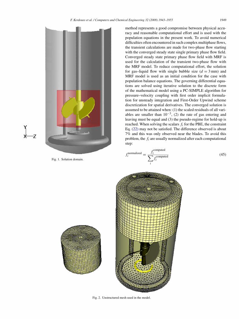
The solution domain for the experimental system investigatedn this work, is shown in Fig. 1. The FLUENT preprocessorAMBIT 2 (2004) is used as geometry and mesh generator.igs. 2 and Fig. 3 show the essential features of the 483,450ybrid cells, generated for the tank consisting of tetrahedral,yramid, wedge and hexahedral cells. The quality of meshes isnalyzed using the skewness criteria (GAMBIT 2, 2004). All theells skewness are below 0.70 which indicate that the mesh iscceptable (GAMBIT 2, 2004). The tank’s domain is discretizedy an unstructured finite volume method, obtained using theolver FLUENT 6.2 (2005) in order to convert the governingquations like continuity and momentum equations to algebraicquations that can be solved numerically. The tank walls, thempeller surfaces and baffles are treated as non-slip boundariesith standard wall functions. At the liquid surface, a small gas
one is added in order to prevent liquid escape from the tankFLUENT 6.2, 2005) and only gas is allowed to escape. The gasow rate at the sparger is defined via inlet-velocity type boundaryondition with gas volume fraction equal to unity. The bubbleiameter at gas orifice (the sparger) is assumed to be uniformnd is calculated from the following correlation (Moo-Young &lanch, 1981; Prince & Blanch, 1990) which is valid for lowas flow rates less than 0.001 m3 s−1 (Perry & Chilton, 1997):
b =(
6σdo
g(ρL − ρG)
)1/3
(44)
here do is the orifice diameter. The single bubble size foundith this correlation (d = 3 mm) is used in the whole tank for
he simulation performed without the PBE model. Multiple Ref-rence Frames Model is used to model the impeller region. MRF
F. Kerdouss et al. / Computers and Chemica
Fig. 1. Solution domain.
Fig. 2. Unstructured mesh
mrpdtwCutfMptoptdaalrE7ps
f
l Engineering 32 (2008) 1943–1955 1949
ethod represents a good compromise between physical accu-acy and reasonable computational effort and is used with theopulation equations in the present work. To avoid numericalifficulties often encountered in such complex multiphase flows,he transient calculations are made for two-phase flow startingith the converged steady state single primary phase flow field.onverged steady state primary phase flow field with MRF issed for the calculation of the transient two-phase flow withhe MRF model. To reduce computational effort, the solutionor gas–liquid flow with single bubble size (d = 3 mm) and
RF model is used as an initial condition for the case withopulation balance equations. The governing differential equa-ions are solved using iterative solution to the discrete formf the mathematical model using a PC-SIMPLE algorithm forressure–velocity coupling with first order implicit formula-ion for unsteady integration and First-Order Upwind schemeiscretization for spatial derivatives. The converged solution isssumed to be attained when: (1) the scaled residuals of all vari-bles are smaller than 10−3, (2) the rate of gas entering andeaving must be equal and (3) the pseudo-regime for hold-up iseached. When solving the scalars fi for the PBE, the constraintq. (22) may not be satisfied. The difference observed is about% and this was only observed near the blades. To avoid thisroblem, the fi are usually normalized after each computationaltep:
used in the model.
normalizedi = f
computedi∑
i
fcomputedi
(45)
1950 F. Kerdouss et al. / Computers and Chemical Engineering 32 (2008) 1943–1955
3
1CgtP6tX4sdaawnalp2ttmembp
Fig. 4. Cell partitions with 4 compute nodes for the bioreactor domain.
Table 2Average wall-clock time per iteration (s) for different parallel test number nodes
A
aintused as compromise between speed up and wall-clock time for
Fig. 3. Flow field in the plane between two baffles.
.9. Parallelization
The computation using a fine mesh for the tank (over,000,000 cells) and the solution of PBE leads to an increase inPU time by many fold and the computing time with only a sin-le serial processor machine may become prohibitive. In ordero reduce the turnaround time, the simulation for the case withBE is parallelized using the parallel solver version of FLUENT.2 (2005). The parallel calculation is performed using a rela-ively inexpensive LINUX cluster of 32 single AMD AthlonP 2800+ 2.08 GHz CPU processor machines with a total of8 gigabytes of memory, connected through a 1000BT gigabitwitch. The parallelization is done by splitting the computationalomain into a number of partitions (Fig. 4). The partition is doneutomatically using the converged transient two-phase flow withsingle size bubble, each partition is send to a compute nodehere the source code is executed simultaneously with the otherodes. The communication among the nodes is performed usingSOCKET communicator which is a FLUENT message passing
ibrary between nodes (FLUENT 6.2, 2005). To evaluate parallelerformance, the case with PBE’s equation is run on 4, 8, 16 and4 compute nodes. Then, the speed-up, which is the ratio of theotal CPU time per the total wall-clock time (elapsed time forhe iterations), is compared for both cases. For a perfect parallel
achine, the total CPU time with n computer nodes would bequal to n times the total wall-clock time. However this improve-
ent in calculation time is reduced by the communication time
etween nodes. While the number of computer nodes increases,arallel processes run slower (Table 2). The parallel efficiency
tem
4 nodes 8 nodes 16 nodes 24 nodes
verage wall-clock time (s) 67 34 18.3 17.5
lso decreases as the ratio of communication to computationncreases (Fig. 5), since for 4 nodes, 8 nodes, 16 nodes and 24odes the speed-up is respectively 97%, 96%, 88% and 62% thanhe ideal case. Considering theses issues 16 computer nodes are
he PBE calculation. The configuration of our cluster makes itfficient for such computational requirements, but it is clear thatuch larger numbers of cells would seriously decrease the effi-
F. Kerdouss et al. / Computers and Chemical Engineering 32 (2008) 1943–1955 1951
cc
4
4
tmcow
w
P
Ie
l
Pe
ficp
k
av
a
f
a1
Table 3Diameters distribution of bubble classes used with the population balanceequations
Fig. 5. Speed-up of parallel compute nodes for the case with PBE.
iency and parallel configurations using much faster inter-nodeommunications would be needed.
. Results and discussions
.1. kLa from measurement and CFD predictions
Dissolved oxygen concentrations measured as a function ofime are used in calculating the experimental overall volumetric
ass transfer coefficient kLa. The increase in dissolved oxygenoncentration is measured until water became saturated withxygen . Hence, the rate of change in oxygen concentrationith liquid phase is given by the following equation:
dCL
dt= kLa(C∗ − CL) (46)
here C∗ is the saturation concentration given by Henry’s Law:
O2 = H · C∗ (47)
ntegration of Eq. (46) with CL = 0 at t = 0 leads to the followingquation:
n
(C∗ − CL
C∗
)= −kLa t (48)
lotting of the left hand-side of Eq. (48) against time gives thexperimental kLa.
Using the CFD simulation, the volumetric mass transfer coef-cient is calculated as the product of the liquid mass transferoefficient kL and the interfacial area a. Based on the Higbie’senetration theory, kL is given as (Dhanasekharan et al., 2005):
L = 2√π
√DO2
(ερL
μL
)1/4
(49)
nd the interfacial area a is given as a function of the local gasolume fraction and local Sauter mean diameter:
= 6αG
d32(50)
Eqs. (49) and (50) are used to predict local and average kLa
rom CFD simulation.The Henry’s constant H and the diffusion coefficient DO2 ,
t 20 ◦C, are respectively 4010 Pa kg−1 m3 and 2.01 ×0−9 m2 s−1 (CRC Handbook, 2002).
x
pri
ig. 6. Contours of gas volume fraction along the plane x = 0 (the same for allistributions of PBE or without PBE).
The Sauter mean diameter is predicted using the populationalance equations with the simulation bubbles are taken from.75 to 12 mm in diameter (Table 3) and divided in classes suchhat vi = 4vi−1. Using a multiblock tank mode, Laakkonen et al.2007) found that more than 80 Classes should be used to min-mize the discretization errors. However for practical reasons,he number of classes was limited to 13 as shown in Table 1.he results are satisfactory for this case.
Fig. 6 shows contours of air volume fraction along the plane
= 0. It can be seen that most of the air rises with low dis-
ersion as the disruptive forces induced by the actual impellerotation are not enough to overcome the buoyancy. This results confirmed by visual observation of the vessel which reveal
PGStudent
Highlight
1952 F. Kerdouss et al. / Computers and Chemical Engineering 32 (2008) 1943–1955
F
taltds
F
F
t
ig. 7. Contours of Sauter diameter d32 along the plane x = 0 (m) 7 Classes.
hat bubbles rise relatively undisturbed through the central arearound the shaft. Figs. 7–10 show the predicted contours of theocal Sauter mean diameter along the plane x = 0 for distribu-
ions of bubbles used. The bubble size increases along the heightue to coalescence in accordance with visual observation. Themallest bubbles are found in the under part of the vessel where
ig. 8. Contours of Sauter diameter d32 along the plane x = 0 (m) 9 Classes.
issra
F
ig. 9. Contours of Sauter diameter d32 along the plane x = 0 (m) 11 Classes.
he gas hold-up is small. The highest local value of kLa, as shownn Figs. 12–16, are found near the impeller where turbulence dis-
ipation rate is high, since turbulence properties determines theurface renewal time for liquid film around bubbles. Fig. 11 rep-esents the kL which doesn’t depend on the number of classesnd Sauter diameter.
ig. 10. Contours of Sauter diameter d32 along the plane x = 0 (m) 13 Classes.
F. Kerdouss et al. / Computers and Chemical Engineering 32 (2008) 1943–1955 1953
F
bwaro
Fw
FC
ig. 11. Contour of kL (the same for all distributions of PBE or without PBE).
The predicted results for the two cases (MRF with single bub-le and MRF with different distributions of PBE) are comparedith the experimental results for the same conditions (Table 4)
nd the same zone. It can be seen that using the PBE gives the bestesults for the kLa compared to the predicted results with onlyne bubble size as the bubble–bubble and bubble–turbulence
ig. 12. Contour of local mass transfer coefficient kLa (s−1) for the case withithout the PBE.
immd
FC
ig. 13. Contour of local mass transfer coefficient kLa (s−1) for the case with 7lasses PBE .
nteractions are taken in account. It is clear that when we useore sizes of bubbles in PBE kLa fits better with the experi-
ental value. We can conclude that 13 Classes seems to get the
esired accuracy.
ig. 14. Contour of local mass transfer coefficient kLa (s−1) for the case with 9lasses PBE .
1954 F. Kerdouss et al. / Computers and Chemical Engineering 32 (2008) 1943–1955
Fig. 15. Contour of local mass transfer coefficient kLa (s−1) for the case with11 Classes PBE .
Fig. 16. Contour of local mass transfer coefficient kLa (s−1) for the case with13 Classes PBE .
Table 4Comparison of CFD predictions of mass transfer coefficient for different distri-bition of PBE with experimental result
A CFD model of gas–liquid dispersion in a agitated vesseloupled with population balance equations is used in order toredict mass transfer in a laboratory scale bioreactor. For suchomplex flows it is shown that using Fluent’s parallel capabili-ies on a relatively small and inexpensive gigabit Linux clusterreatly accelerates the calculation. The model predicts spatialistribution of gas hold-up, Sauter mean bubble diameter andass transfer coefficient. The numerical results are comparedith experimental data for mass transfer coefficient and showood agreement. The mathematical development of the two-hase aspects and computational techniques of the model isontinuing in order improve the overall speed of the calcula-ions, as well as accounting for non-Newtonian behavior of the
edia.As a final conclusion using PBE gives better accuracy than
raditional method with a one mean diameter. When we compareetween what we gain in accuracy when we double the distribu-ion of bubbles and the time and computtational time used wean note that it is not so useful to use more than 13 Classes.
cknowledgments
The projet was partially supported by the National Sciencend Engineering Research Council of Canada, NSERC. The con-ributions of Pr. P. Vermette, responsible of the biotechnologicalngineering first year’s project, and assistant I. Arsenault, forer technical assistance are also gratefully acknowledged.
eferences
lopaeus, V., Koskinen, J., & Keskinen, K. I. (1999). Simulation of the popu-lation balances for liquid–liquid systems in a nonideal stirred tank. Part-1:Description and qualitative validation of the model. Chemical EngineeringScience, 54, 5887–5889.
lopaeus, V., Koskinen, J., Keskinen, K. I., & Majander, J. (2002). Simulationof the population balances for liquid–liquid systems in a nonideal stirredtank. Part-2: Parameter fitting and the use of the multiblock model for densedispersions. Chemical Engineering Science, 57, 1815–1825.
akker, A., & Van Den Akker, H. E. A. (1994). A computational model forthe gas–liquid flow in stirred reactors. Transactions of IChemE, 72(Part A),
594–606.
ove, S., Solberg, T., & Hjertager, B. H. (2005). A novel algorithm forsolving population balance equations: The parallel parent and daughterclasses. Derivation, analysis and testing. Chemical Engineering Science,60, 1449–1464.
emica
C
C
C
D
D
E
F
F
G
H
H
I
J
K
K
K
K
L
L
L
L
L
L
L
M
M
M
M
M
M
M
M
P
P
RR
R
R
S
S
T
V
F. Kerdouss et al. / Computers and Ch
hen, P., Dudukovic, M. P., & Sanyal, J. (2005a). Numerical simulation ofbubble columns flows: effect of different breakup and coalescence closures.Chemical Engineering Science, 60, 1085–1101.
hen, P., Dudukovic, M. P., & Sanyal, J. (2005b). Three-dimensional simula-tion of bubble column flows with bubble coalescence and breakup. AICHEJournal, 51(3), 696–712.
RC Handbook. (2002). Handbook of Chemistry and Physics (83rd ed.). BocaRaton, FL, USA: CRC Press LLC.
een, N. G., Solberg, T., & Hjertager, B. H. (2002). Flow generated by an aeratedRushton impeller: Two-phase PIV experiments and numerical simulations.The Canadian Journal of Chemical Engineering, 80, 1–15.
hanasekharan, K., Sanyal, J., Jain, A., & Haidari, A. (2005). A generalizedapproach to model oxygen transfer in bioreactors using population bal-ances and computational fluid dynamics. Chemical Engineering Science,60, 213–218.
lgobashi, S. E., & Rizk, M. A. (1989). A two-equation turbulence model for dis-persed dilute confined two-phase flows. International Journal of MultiphaseFlow, 15(1), 119–133.
LUENT 6.2. (2005). User’s Manual to FLUENT 6.2, Centrera Resource Park,10 Cavendish Court, Lebanon, USA: Fluent Inc.
riberg, P. C. (1998). Three-dimensional modeling and simulations of gas–liquidflows processes in bioreactors. Ph.D. Thesis. Porsgrum, Norway: NorwegianUniversity of Science and Technology.
AMBIT 2. (2004). User’s Manual to GAMBIT 2. Centrera Resource Park, 10Cavendish Court, Lebanon, USA: Fluent Inc.
agesaether, L., Jakobsen, H. A., Hjarbo, K., & Svendsen, H. (2000). A coales-cence and breakup module for implementation in CFD codes. In EuropeanSymposium on Computer Aided Process Engineering, Vol. 10 (pp. 367–372).
jertager, B. H. (1998). Computational fluid dynamics (CFD) analysis of mul-tiphase chemical reactors. Trends in Chemical Engineering, 4, 45–91.
shii, M., & Zuber, N. (1979). Drag coefficient and relative velocity in bubbly,droplet or particulate flows. AIChE Journal, 25(5), 843–855.
enne, M., & Reuss, M. (1999). A critical assessment on the use of k–e turbulencemodels for simulation of the turbulent liquid flow induced by Rushton-turbine in baffled stirred-tank reactors. Chemical Engineering Science, 54,3921–3941.
erdouss, F., Bannari, A., & Proulx, P. (2006). CFD modeling of gas disper-sion and bubble size in a double turbine stirred tank. Chemical EngineeringScience, 61, 3313–3322.
erdouss, F., Kiss, L., Proulx, P., Bilodeau, J. F., & Dupuis, C. (2005). Mixingcharacteristics of an axial flow rotor: Experimental and numerical study.International Journal of Chemical Reactor Engineering, 3, A35.
hopkar, A. R., Rammohan, A. R., Ranade, V. V., & Dudukovic, M. P. (2005).Gas–liquid flow generated by a Rushton turbine in stirred vessel: CARPT/CTmeasurements and CFD simulations. Chemical Engineering Science, 60,2215–2229.
umar, S., & Ramkrishna, D. (1996). On the solution of population balanceequations by discretization—I. A fixed pivot technique, 51, 1311–1332.
aakkonen, M., Alopaeus, V., & Aittamassa, J. (2006). Validation of bubblebreakage, coalescence and mass transfer models for gas–liquid dispersionin agitated vessel. Chemical engineering science, 61, 218–228.
aakkonen, M., Moilanen, P., Alopaeus, V., & Aittamassa, J. (2006). Dynamicmodeling of local reaction conditions in an agitated aerobic fermenter.AICHE Journal, 52(5), 1673–1689.
aakkonen, M., Moilanen, P., Alopaeus, V., & Aittamassa, J. (2007). Model-ing local bubble sizedistributions in agitated vessels. Chemical EngineeringScience, 62, 721–740.
ane, G. L., Schwarz, M. P., & Evans, G. M. (2002). Predicting gas–liquid flow ina mechanically stirred tank. Applied Mathematical Modeling, 26, 223–235.
V
l Engineering 32 (2008) 1943–1955 1955
ane, G. L., Schwarz, M. P., & Evans, G. M. (2005). Numerical modellingof gas–liquid flow in stirred tank. Chemical Engineering Science, 60,2203–2214.
uo, J. Y., Issa, R. I., & Gosman, A. D. (1994). Prediction of impeller inducedflows in mixing vessels using multiple frames of reference. In IchemESymposium Series, Institution of Chemical Engineers, vol. 136 (pp. 549–556).
uo, H., & Svendsen, H. F. (1996). Theoretical model for drop and bubblebreakup in turbulent dispersions. AIChE Journal, 42(5), 1225–1233.
cGraw, R. (1997). Description of aerosol dynamics by the quadrature methodof moments. Aerosol Science and Technology, 27, 255–265.
archisio, D. L., & Fox, R. O. (2005). Solution of population balance equationsusing the direct quadrature method of moments. Journal of Aerosol Science,36, 43–73.
archisio, D. L., Pikturna, J. T., Fox, R. O., & Vigil, R. D. (2003). Quadraturemethod ofmoments for population-balance equations. AIChE Journal, 49,1266–1276.
archisio, D. L., Vigil, R. D., & Fox, R. O. (2003). Quadrature method ofmoments for aggregation-breakage processes. Journal of Colloid and Inter-face Science, 258, 322–334.
icale, G., Brucato, A., & Grisafi, F. (1999). Prediction of flow fields in adual-impeller stirred tank. AICHE Journal, 45(3), 445–464.
oo-Young, M., & Blanch, H. W. (1981). Design of biochemical reactors. Adv.Biochem. Eng., 19, 1–69.
orud, K. E., & Hjertager, B. H. (1996). LDA measurements and CFD modelingof gas–liquid flow in a stirred vessel. Chemical Engineering Science, 51,233–249.
udde, R., & Simonin, O. (1999). Two- and three-dimensional simulations of abubble plume using a two-fluid model. Chemical Engineering Science, 54,5061–5069.
erry, R. H., & Chilton, C. H. (1997). Perry’s chemical engineer’s handbook(2nd ed.). USA: McGraw-Hill.
rince, M. J., & Blanch, H. W. (1990). Bubble coalescence and break-up inair-sparged bubble columns. AIChE Journal, 36(10), 1485–1499.
amkrishna, D. (2000). Population Balances. San Diego: Academic Press.anade, V. V., & Deshpande, V. R. (1999). Gas–liquid flow in stirred vessels:
Trailing vortices and gas accumulation behind impeller blades. ChemicalEngineering Science, 54, 2305–2315.
anade, V. V. (1997). An efficient computational model for simulating flow instirred vessels: A case of Rushton Turbine. Chemical Engineering Science,52, 4473–4484.
utherford, K., Lee, K. C., Mahmoudi, S. M. S., & Yianneskis, M. (1996).Hydrodynamic characteristics of dual rushton impeller stirred vessels.AICHE Journal, 42(2), 332–346.
affman, P. G., & Turner, J. S. (1956). On the collision of drops in turbulentclouds. Journal of Fluid Mechanics, 1, 16–30.
anyal, J., Marchisio, D. L., Fox, R. O., & Dhanasekharan, K. (2005). Onthe comparaison between population balance models for CFD simulationof bubble columns. Industrial Engineering and Chemical Research, 44,5063–5072.
abor, G., Gosman, A. D., & Issa, R. I. (1996). Numerical simulation of the flowin a mixing vessel stirred by a Rushton Turbine. IChemE Symposium Series,140, 25–34.
anni, M. (2000). Approximate population balance equations for aggregation-
breakage processes. Journal of Colloid and Interface Science, 221, 143–160.
enneker, B. C. H., Derksen, J. J., & Van Den Akker, H. E. A. (2002). Populationbalance modeling of aerated stirred vessels based on CFD. AICHE Journal,48(4), 673–684.