1 2 3 4 5 6 7 8 9 10 11 12 13 14 15 16 17 18 19 20 Kinematics of fault-related folding derived from a sandbox experiment Sylvain Bernard 1,* , Jean Philippe Avouac 1 , Stéphane Dominguez 2 , Martine Simoes 1, ** 1 Tectonics Observatory, California Institute of Technology, Pasadena, USA. 2 Laboratoire Dynamique de la Lithosphère, ISTEEM, Montpellier, France. * now at Laboratoire de Géologie, Ecole Normale Supérieure, Paris, France. ** now at Géosciences Rennes, Université Rennes 1, France Abstract We analyze the kinematics of fault-tip folding at the front of a fold-and-thrust wedge using a sandbox experiment. The analog model consists of sand layers intercalated with low friction glass bead layers, with a total thickness h = 4.8 cm, deposited in a glass sided experimental device. A computerized mobile backstop induces progressive horizontal shortening of the sand layers and consequently thrust fault propagation. Active deformation at the tip of the forward propagating basal décollement is monitored along the cross section with a high resolution CCD camera, and the displacement field between pairs of images is measured from the optical flow technique. In the early stage, when cumulative shortening is less than about h/10, slip along the décollement tapers gradually to zero and the displacement gradient is absorbed by 1
Transcript
1
2
3
4
5
6
7
8
9
10
11
12
13
14
15
16
17
18
19
20
Kinematics of fault-related folding derived
from a sandbox experiment
Sylvain Bernard1,*, Jean Philippe Avouac1, Stéphane Dominguez2, Martine
Simoes1, **
1 Tectonics Observatory, California Institute of Technology, Pasadena, USA.
2 Laboratoire Dynamique de la Lithosphère, ISTEEM, Montpellier, France.
* now at Laboratoire de Géologie, Ecole Normale Supérieure, Paris, France.
** now at Géosciences Rennes, Université Rennes 1, France
Abstract
We analyze the kinematics of fault-tip folding at the front of a fold-and-thrust wedge
using a sandbox experiment. The analog model consists of sand layers intercalated with low
friction glass bead layers, with a total thickness h = 4.8 cm, deposited in a glass sided
experimental device. A computerized mobile backstop induces progressive horizontal shortening
of the sand layers and consequently thrust fault propagation. Active deformation at the tip of the
forward propagating basal décollement is monitored along the cross section with a high
resolution CCD camera, and the displacement field between pairs of images is measured from
the optical flow technique. In the early stage, when cumulative shortening is less than about h/10,
slip along the décollement tapers gradually to zero and the displacement gradient is absorbed by
1
1
2
3
4
5
6
7
8
9
10
11
12
13
14
distributed deformation of the overlying medium. In this stage of detachment-tip folding,
horizontal displacements decrease linearly with distance towards the foreland. Vertical
displacements reflect a nearly symmetrical mode of folding, with displacements varying linearly
between relatively well-defined axial surfaces. When the cumulative slip on the décollement
exceeds about h/10, deformation tends to localize on a few discrete shear bands at the front of the
system, until shortening exceeds h/8 and deformation gets fully localized on a single emergent
frontal ramp. The fault geometry subsequently evolves to a sigmoid shape and the hanging wall
deforms by simple shear as it overthrusts the flat-ramp system. As long as strain localization is
not fully established the sand layers experience a combination of thickening and horizontal
shortening which induce gradual limb rotation. The observed kinematics can be reduced to
simple analytical expressions that can be used to restore fault-tip folds, relate finite deformation
to incremental folding, and derive shortening rates from deformed geomorphic markers or
growth strata.
2
1
2
3
4
5
6
7
8
9
10
11
12
13
14
15
16
17
1. Introduction
Abandoned fluvial or alluvial terraces, as well as growth strata can be used to determine
incremental deformation associated with active folds [e.g., Rockwell, et al., 1988; Suppe, et al.,
1992; Hardy and Poblet, 1994; Molnar, et al., 1994; Hardy, et al., 1996; Storti and Poblet, 1997;
Lavé and Avouac, 2000; van der Woerd, et al., 2001; Thompson, et al., 2002]. If a unit can be
traced all the way across a given fold it can be used to estimate uplift since its deposition, and
then to derive the corresponding average shortening from a mass balance calculation
[Chamberlin, 1910; Epard and Groshong, 1993] (Figure 1). Although this geometrical approach
can be used to estimate cumulative shortening, it can only rarely be applied to geomorphic
markers since a terrace record is often discontinuous and buried below younger sediments in the
foreland or in piggyback basins. An alternative approach consists in fitting the terrace record
from a model of folding constrained from pre-growth strata (structural measurements or
subsurface data). This approach has been applied to fault-bend folds (Figure 2A) assuming that
the hanging wall deforms by flexural-slip folding [Lavé and Avouac, 2000; Thompson, et al.,
2002]. In such a case, where both bed length and thickness are constant, the local uplift U
relative to the footwall, assumed rigid, obeys
18
19
20
21
22
23
)(sin)()()( xzRbxixU (1)
where x is the distance along the section line i(x) is the river incision since terrace abandonment;
b is the base level change since terrace abandonment (positive upward); (x) is the local bedding
dip angle; and R(z) is the horizontal shortening since terrace abandonment of the layer at
elevation z, which crops out at distance x from the trailing edge of the section (Figure 1). Base
level change may lead to either entrenchment (b<0) or aggradation (b>0) in the foreland. On the
3
sketch in Figure 1, we have assumed no bed-parallel shear away from the fault zone, hence R is
independent of z. In that case, estimating R does not require a continuous terrace profile and it is
sufficient to use only a few independent estimates of the entrenchment rate at places with
different dip angles in the zone where the bedding is already parallel to the fault plane (i.e.
backlimb of the fold represented in Figure 1). In principle, estimates of incision rate at at least
two points with different dip angles are necessary to derive both R and b [Thompson, et al.,
2002]. When sufficiently complete terrace records are available, the relationship expressed by (1)
is testable since it predicts that uplift and the sinus of the local bedding dip angle, sin( , are
proportional. Irrespective of the geomorphic record, it is important to note that this approach
does not apply all along the profile of the fold, but only where the bedding is parallel to the fault
plane (Figures 1 and 2B).
1
2
3
4
5
6
7
8
9
10
11
12
13
14
15
16
17
18
19
20
21
22
23
Fault-tip folds can develop by distributed pure shear, with requisite bed length and
thickness changes associated with limb rotation [Dahlstrom, 1990; Erslev, 1991; Poblet and
McClay, 1996; Mitra, 2003], or by kink-band migration and bed-parallel simple shear, as in the
case of fault-propagation folds [Suppe and Medwedeff, 1990; Mosar and Suppe, 1992]. In either
case, beds near the surface are not everywhere parallel to the thrust fault at depth, so that
equation (1) does not hold in places like the fold forelimb in Figure 1. Figure 2B shows a number
of acceptable kinematic models of fault-tip folds, all based on the assumption of mass
conservation. Most of these models are commonly used to guide interpretation of structural
measurements or seismic profiles [Erslev, 1991; Mosar and Suppe, 1992; Wickham, 1995; Storti
and Poblet, 1997; Allmendinger, 1998; Allmendinger and Shaw, 2000; Brooks, et al., 2000;
Zehnder and Allmendinger, 2000; Mitra, 2003]. In contrast to these purely geometric models,
some authors have explored the possibility of modeling folds from the theory of elastic
4
dislocations in an elastic half-space [Myers and Hamilton, 1964; King, et al., 1988; Stein, et al.,
1988; Ward and Valensise, 1994; Savage and Cooke, 2004]. Although any of these various fold
models might be used to analyze growth strata or deformed alluvial terraces and retrieve the
kinematic history of folding, two difficulties generally arise. One is that the choice of a
kinematic model is not straightforward, even when growth strata geometry is well constrained.
The other is that the mathematical implementation of these models and the adjustment to field
data is generally not simple. For these reasons, we seek a simple alternative relationship linking
local uplift and/or bedding tilt to structural geometry. This relationship must be applicable across
an entire structure and must be grounded in realistic fold kinematics or mechanics. For this
purpose, we analyze folding produced in an analogue experiment to derive some kinematic
model.
1
2
3
4
5
6
7
8
9
10
11
12
13
14
15
16
17
18
19
20
21
22
It has been observed that the formation of the most frontal ramp in analogue models of
wedge mechanics [Dominguez, et al., 2001] is preceded by a phase of distributed deformation
which resembles fault-tip folding. We therefore focused the present study on this particular
phase, assuming it can be considered to simulate the kinematics of the early stage of fault-related
folding at the natural scale. With this aim, we used a new experimental set-up that allows
accurate measurements of fault slip kinematics and of the associated deformation field
[Dominguez, et al., 2003].
We first present the experimental set-up and the principles of the approach. We then
describe in detail the evolution of incremental deformation during a representative experiment
selected among more than 10 performed experiments, and derive some simple analytical
approximations. Finally, we propose and test a procedure that can be used to restore incremental
5
1
2
3
4
5
6
7
8
9
10
11
12
13
14
15
16
17
18
19
20
21
22
or cumulative deformation across fault-tip folds. All variables introduced in the analysis are
listed and defined in Table 1.
2. Experimental Set-up
The physical properties of dry sand and glass beads ( s ~ 30°, low cohesion, time
independent mechanical behaviour) make them good analogue materials to simulate brittle
deformation of the upper crust at the laboratory scale [e.g. Malavieille, 1984; Mulugeta, 1988;
Mulugeta and Koyi, 1992; Koyi, 1995; Gutscher, et al., 1998; Dominguez, et al., 2000; Adam et
al, 2005; Konstantinovskaia and Malavieille, 2005]. Experiments where the layers are overlying
a rigid basement and are subjected to horizontal shortening produce a self-similar accretionary
prism analogous to accretionary prisms formed along subduction zones or in intracontinental
fold-and-thrust belts [Chapple, 1978; Davis, et al., 1983; Lallemand, et al., 1994; Gutscher, et
al., 1998]. These experiments lead to the formation of imbricated thrust sheets that gradually
accrete to the wedge as the detachment propagates forward. In the absence of cohesion this
process and the resulting geometries are scale independent. However, given the estimate of the
cohesion of the material used in this experiment (Co<50 Pa) and the typical cohesion of crustal
rocks (Co>20MPa [Lallemand, et al., 1994; Schellart, 2000], the scaling factor can be estimated
to about 105. Accordingly, 1 cm in the model is equivalent to about 1 km in nature.
The model box is 20 cm wide and 100 cm long and equiped with transparent side walls
treated to reduce friction [Dominguez et al., 2001]. The model comprises 6 sand layers, each 6-7
mm thick, intercalated with 5 glass bead layers, each 2 mm thick. The total model thickness, h, is
4.8 cm. We use this layering to simulate natural lithologic intercalations and stratigraphic
6
1
2
3
4
5
6
7
8
9
10
11
12
13
14
15
16
17
18
19
20
21
22
23
discontinuities, and to facilitate layer parallel shear, a process which is thought to be key to
folding of sedimentary layers at the natural scale.
The sand and glass bead layers are deformed in front of a moving backstop activated by a
step motor at a constant velocity of 235 ± 10 μm per minute (1.4 cm/h (Figure 3). The cohesion
and friction angle of the materials was provided by the manufacturers (SIFRACO and
EYRAUD) and also measured in our laboratory [Krantz, 1991; Jolivet, 2000; Schellart, 2000].
The sand has a fluvial origin with irregularly rounded grain shapes and sizes from 150 to 300
μm. Its internal friction angle is 30˚ to 35˚ (tan( s)=0.6 to 0.7) and its cohesion is low (Co < 50
Pa). The glass beads are SiO2-Na2O, cohesionless microspheres with grain sizes ranging from
50 to 150 μm and an internal friction angle between 20˚ and 25˚ (tan g=0.35 to 0.45). The model
is built on a 2 cm thick, horizontal ( =0) polyvinyl chloride (PVC) plate. The basal friction along
the sand/unpolished PVC interface is 21˚±4° (tan( b= 0.38) [Jolivet, 2000].
Our experimental set-up was designed so as to measure, with the maximum possible
accuracy, the deformation at the tip of the basal detachment and the formation of a new thrust
fault at the front of the wedge. In order to avoid episodic re-activation of older internal faults and
force the deformation to be localized at the very front of the wedge, we started the experiment
with a 10° pre-deformation sandwedge. In experiments run with the same layering as the one
described here we observed the formation of a wedge with a slope of 8-9° which is
approximately the critical slope of about 8° of a homogeneous wedge predicted from the critical
wedge theory given the value of the basal friction angle, b, of 21° and the value of the internal
friction angle, s, of 30° for the sand mass [Davis, et al., 1983]. This shows that the layering does
not modify significantly the mechanical behavior of the accretionary wedge and that coulomb
wedge theory can still be applied.
7
1
2
3
4
5
6
7
8
9
10
11
12
13
14
15
16
We focus on the foreland edge of the wedge, which grows by the forward propagation of
the basal décollement. This part of the experiment is located about 15 cm from the backstop and,
to ensure maximum spatial resolution, is the only portion of the experiment monitored with the
video system (box in Figure 3). By comparing the imposed displacement of the backstop with
displacements measured within the zone monitored by the video system, we find that during the
selected experiment about 98% of the shortening is absorbed by internal deformation within the
monitored frame. Photographs are taken with a constant sampling rate of 1 image/minute with a
6.3 megapixels CCD camera. The pixel size is 80 by 80 m². Given that the backstop velocity
and the sampling rate are constant, the incremental shortening between two successive images is
constant and equals 235 +/- 10 m. The displacement field between two successive images is
measured from the optical flow technique, which was introduced by Horn and Schunk [1980]
and commonly used in remote sensing and image processing for robotic applications. It applies
to images with a brightness pattern that evolves only due to deformation of the medium, as is the
case of our experiment. The technique allows a subpixel accuracy and appears more powerful
than more recent correlation techniques such as Particle Imaging Velocimetry [Adam, et al.,
2005]. It is based on the fact that the image F at time t+dt, can be written:
17 dXtFtFdttF )()()( (2)
where dX is the displacement field and F(t) is the spatial gradient of image F(t). Equation (2)
is only an approximation because higher order terms in the Taylor-Lagrange development are
neglected. The gradient is estimated from Rider’s method [Press, et al., 1995]. The technique
was first applied to the analysis of sandbox experiments by Dominguez, et al. [2001].
18
19
20
21
22
23
The displacement field varies smoothly and the signal to noise ratio is better when it is
measured over few images (typically over 2-3 images). The correlation window is 32*32 pixels,
8
1
2
3
4
5
6
7
8
9
10
11
12
13
14
15
16
17
18
19
20
21
22
23
and is moved by increments of 8 pixels across the whole image. The displacement field thus
contains 350*149 independent measurements, with a sampling (or spatial) resolution of 640 m.
Based on calibration tests, errors on measurements are statistically estimated to be less than 5 %.
The horizontal and vertical components of the displacements are plotted separately and used to
generate various representations such as displacement vectors or incremental deformation of a
virtual grid (Figures 3 and 4). Because the measurements are made from pairs of images
separated by variable time lags, incremental displacements are normalized by dividing them by
the number of time steps (1 step corresponding to two successive images). Displacements are
thus expressed in millimeters per step (mm/step), a step corresponding to a shortening of 235 +/-
10 m, and are thus equivalent to normalized velocities. For our analysis we examine profiles
across the horizontal and vertical displacement fields at different depths above the décollement.
Surface processes are not simulated in the model. Therefore, the analogue experiment
does not directly reproduce growth strata nor deformed terraces. However, the mathematical
description of folding derived from this experiment, as detailed below, can easily be used to
simulated the expected geometry of growth strata or terraces [Simoes, et al., this issue; Daeron,
et al., this issue].
3. From detachment-tip folding to ramp overthrusting
Deformation within the domain covered by the imaging system starts to become
significant only after about image 10, which corresponds to 2.3 mm of shortening, or 5% of the
initial thickness of the sand layers (h/20). Prior to this, deformation is entirely accommodated
closer to the backstop, outside the area covered by the camera. Following this initial phase of
shortening, the evolution of deformation can be divided into two main stages that are the focus of
our analysis. The first stage comprises distributed deformation and tip-line folding above the
9
1
2
3
4
5
6
7
8
9
10
11
12
13
14
15
16
17
18
19
20
21
22
23
foreland edge of the horizontal basal detachment. The second deformation stage occurs after a
brief transitional phase of strain localization, and consists of upward propagation of the
detachment tip and of formation of a mature frontal thrust ramp. Hanging-wall material is
subsequently transported along this new fault surface.
During the first stage of deformation, horizontal velocities decrease linearly with distance
away from the backstop, and vertical velocities show a nearly symmetrical, trapezoidal pattern of
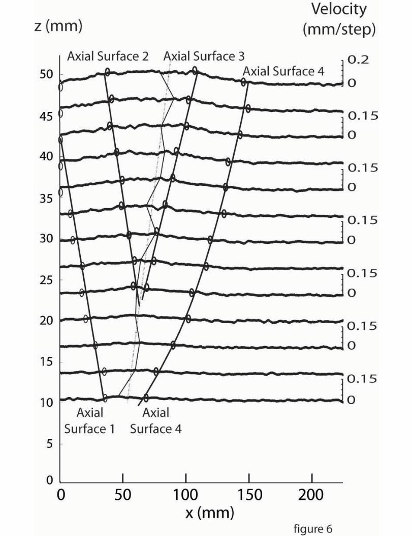
uplift (Figure 5A). We separate the uplift pattern into domains in which incremental uplift varies
linearly with horizontal distance, and interpret the boundaries of these domains as fold axial
surfaces. The position of each of these surfaces was determined by the maximum change in slope
of the uplift rate versus distance curve as calculated in several different horizons (Figure 6). The
analysis of the evolving velocity fields during this stage of deformation allowed us to study the
four identified axial surfaces kinematic behaviour.
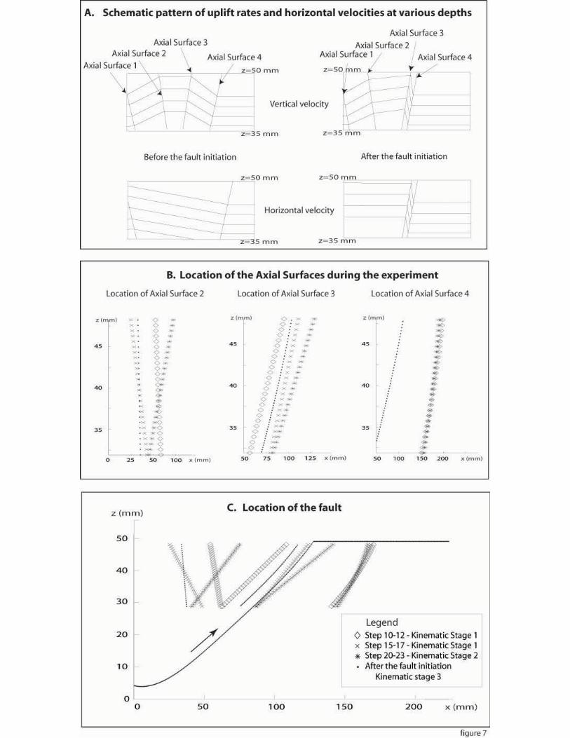
The two outer axial surfaces (labelled 1 and 4 in Figure 7) initiate and remain in their
same positions throughout the first stage of deformation. Axial surface 4 marks the frontal limit
of the deforming zone and appears to be fixed to both the footwall and hanging wall, essentially
acting as a foreland pin line. The discontinuity in the horizontal velocity field places this pin line
30 mm further to the foreland than the discontinuity in the vertical displacement field, suggesting
there is a measurable, but small volume loss in the foreland adjacent to the growing fold. We
believe this volume loss is a specific feature of the analogue model, and most likely results from
a reorganization of sand grain packing that would not occur in a natural setting. The most
hinterland axial surface, number 1, is also fixed to the footwall, but hanging-wall material
appears to migrate through it as shortening continues (Figure 7B). Axial surfaces 2 and 3
immediately bound the fold crest, and are only recognized by discontinuities in the vertical
10
1
2
3
4
5
6
7
8
9
10
11
12
13
14
15
16
17
18
19
20
21
22
23
velocity field (Figure 7A). These surfaces move slightly and/or change orientation during
continued shortening, suggesting they are loosely fixed to the hanging wall (Figure 7B).
Throughout the first stage of deformation, the sand layers in the fold limbs rotate and experience
some component of pure shear.
The end of the first deformation stage is marked by a short, transient stage of strain
localization that precedes ramp overthrusting. In this particular experiment at a cumulative
shortening of 4.2 mm, the deformation gradually focused along two discrete shear bands, each
dipping approximately 25˚ toward the hinterland. Although the shear bands occur as prominent
features in the horizontal displacement field (Figure 4B and 5B), they accommodate less than
30% of the total deformation. With continued shortening the more internal shear band, which
approximately coincides with axial surface 3 defined in the vertical displacement field, tends to
become dominant and evolves into a well-developed thrust fault connecting the basal
décollement to the surface (Figures 4C and 5C). Formation of this frontal thrust ramp induces a
significant change of model deformation kinematics and marks, then, the end of the fault tip
stage.
At the beginning of the second stage of deformation, when the cumulative shortening
typically exceeds about 6 mm, or roughly 13% of the initial thickness of the sand layers (h/8), a
prominent thrust ramp exists at the front of the sand wedge (Figures 4C, 4D, 5C and 5D). The
footwall subsequently stops deforming and all the horizontal shortening is taken up by slip on
this shear zone, which acquires a stable sigmoid geometry. The hanging wall is then thrusted
over the ramp with some internal deformation to accommodate the flat-to-ramp geometry. Axial
surface 1 remains fixed to the footwall whereas axial surface 2 is fixed to the hanging wall and is
passively transported along the fault. Thereafter, the velocity field remains constant, because the
11
1
2
3
4
5
6
fault geometry ceases to evolve. In general, the kinematics of the second stage of deformation is
very similar to those of a simple ramp anticline as predicted by fault-bend folding theory [Suppe
1983] (Figure 2A).
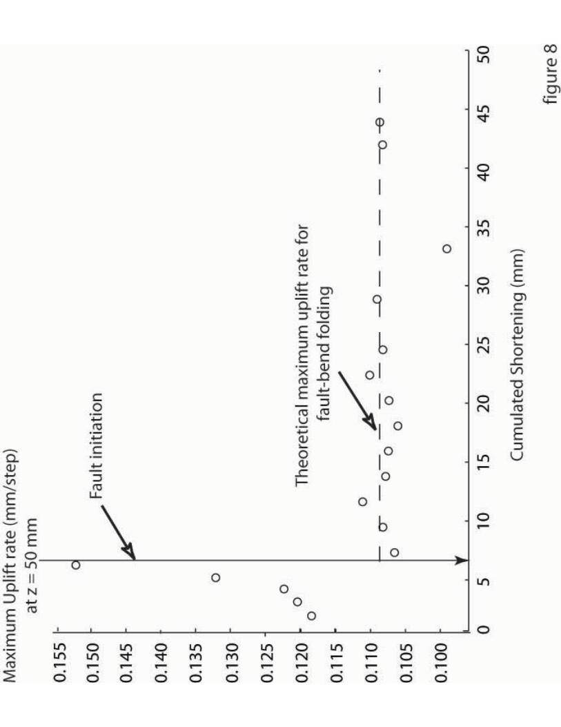
Figure 8 shows how the maximum uplift rate, Umax, varies during a complete experiment.
Before deformation gets localized, maximum uplift rate is observed to increase gradually and
may be as large as twice the value predicted by fault-bend folding theory:
maxmax rU sin (3)7
8
9
10
11
12
13
14
15
16
17
18
19
20
21
22
23
where r is the shortening rate and max is the maximum dip angle of the fault, here about 25˚.
This result is consistent with little internal deformation within the sand layers, and demonstrates
that care must be taken when inferring shortening rates from uplift rates during the detachment-
tip folding phase of deformation that is prior to the formation of the thrust ramp.
4. Analytical representations of surface uplift and horizontal velocity during fault-tip
folding.
Vertical displacements are described from linear segments connecting the four axial
surfaces (Figures 5 and 7). The axial surfaces are generally well defined from the profiles run at
elevations above about 25 mm, but are generally more difficult to track closer to the décollement
where vertical displacements are smaller. The geometry of the first axial surface is not always
well determined since it extends outside the image. Horizontal displacements vary linearly with
horizontal distance between two bounding axial surfaces (Figure 5).
During the first detachment-tip folding stage of deformation, we observe that horizontal
velocity, V, decreases linearly with x, and tapers to zero at ~ 30 mm ahead of the axial surface 4
(Figure 4A and 5A). Incremental horizontal displacements can be described by
12
xzzrV )(1)( (4) 1
2 where r(z) is the horizontal incremental shortening at the back of the structure and
)(1)( zWz h , and Wh(z) is the distance between axial surfaces 1 and 4. 3
4
5
Because the maximum uplift rate scales linearly with the initial datum elevation, z (Figure 9), we
may write:
6
7
8
9
10
zUmax (5)
In the ideal case of a zero thickness décollement, the parameter should be equal to zero
because no uplift would be observed at the level of the décollement. This parameter μ is not zero
in our experiment because the décollement is a shear zone of finite thickness.
In addition, as shown in Figure 9, the uplift profile at each depth obeys
X
UU max 6)11
12
13
where U is the difference in uplift at two points separated by a horizontal distance X. Since
Umax depends linearly on z, we get
,zX
U )14
15
16
which implies that the pattern of incremental uplift in each dip domain between the axial
surfaces can be written as
),(zxzxU (8) 17
18
19
20
where the parameters depend on the considered dip domain. This simple
parameterization yields a good fit to the data (Figure 10). For easier use, equation (8) can be
rewritten for each domain, i,
13
1
2
3
4
5
6
7
8
9
10
11
12
13
14
151617
18
19
20
21
22
23
24
)(),(),( iii xxzzxUzxU , (9)
where i is a constant parameter for each dip domain i considered; the term U(xi,z) corresponds
to the vertical increment within the dip domain (i-1) at the horizontal position xi of the axial
surface shared by consecutive dip domains i and (i-1), and allows for continuity of vertical
displacements from one dip domain to the next one. Since the surface area of the deforming
domain is approximately constant, U(x,z) depends uniquely on the parameters in equation (9) and
on the position of the two axial surfaces defined from the horizontal displacements. The
predicted horizontal velocity obtained from that assumption is in quite good agreement with the
measurements (Figure 10A). During the transition from the initial stage of distributed
deformation to ramp anticline formation, horizontal displacements need a more complex
formulation. A reasonable fit to the data is however still obtained by assuming again mass
conservation and linear functions between axial surfaces (Figure 10B).
5. Comparison with other models of fault-related folding
5.1 Comparison with an elastic dislocation model
We discuss first the possibility of modeling the observed kinematics from dislocations
embedded in an elastic half-space [Okada, 1985]. Although the deformation observed in the
experiment is not recoverable, hence non-elastic, it might be argued that this kind of model
might provide a reasonable approximation to the velocity field [e.g., Ward and Valensise, 1994].
Following Ward and Valensise [1994] we have imposed a coefficient of Poisson of 0.5 to insure
conservation of volume. We found it impossible to correctly predict simultaneously the vertical
and horizontal velocities from this approach (Figures 11 and 12). We reached the same
conclusion while analyzing the stage of fault-tip folding and the stage of ramp overthrusting. In
14
1
2
3
4
5
6
78
9
10
11
12
13
14
15
16
17
18
19
20
21
22
both cases, we find that slip rates derived from modeling the uplift pattern using elastic
dislocations would be overestimated. It is generally possible to obtain a reasonable fit to the the
profile of uplift rate at the surface, or in a naturale case to deformed seismic reflectors from this
approach, , but inferences of fault geometry at depth and any displacement rates might be biased
and should be considered with caution.
5.2 Comparison with trishear folding
The kinematics observed in our experiments show similarities with the trishear fault-
propagation model [Erslev, 1991]. In the trishear model, a single fault expands outward into a
triangular zone of distributed shear. An unlimited number of velocity fields and shapes of the
triangular zone can be generated by varying the propagation-to-slip ratio (P/S), which determines
how rapidly the tip line propagates relatively to the slip on the fault itself [Allmendinger, 1998;
Allmendinger and Shaw, 2000; Zehnder and Allmendinger, 2000].
In the first phase results from distributed shear in a domain delimited by the two
bounding hinges. Shear is not homogeneous and the deforming domain is not exactly triangular.
As formulated in previous studies the trishear models requires in addition that the fault dip angle
lies between the dip angles of the two boundaries of the triangular zone of distributed shear. As a
result, it is not possible to model distributed shear above the tip of a décollement. Hence the
model doesn’t apply directly to the first phase. The trishear model might be adapted to that case
but here we rather opted for the formulation described above (equation (4) and (9)) which
ignores the propagation of the décollement.
15
1
2
3
4
567
8
9
10
11
12
13
14
15
16
17
Deformation during the stage of propagation of the frontal ramp propagation is close to a
trishear fold mechanism although there is no clear indication in our experiment of propagation of
the tip of the ramp during this transient stage of strain localization (Figure 2 B4).
5.3 Comparison with the fault-bend fold model
Once the frontal ramp has propagated up to the surface (when cumulative regional
shortening exceeds h/8) the system evolves toward a ramp anticline. In this case, the uplift rate
pattern is fully determined by the shortening rate, r, and the fault geometry, which controls the
position of the axial surfaces. A possible kinematic model would be that the hanging wall
deforms by bedding plane slip according to the fault-bend folding model [Suppe, 1983], which
assumes the conservation of the length and thickness of the sand layers. Here, we test whether
this model can be used to model the kinematics of folding in the stage of ramp-anticline folding.
In such a case, equation (1) would hold as soon as the sand layers become parallel to the fault, as
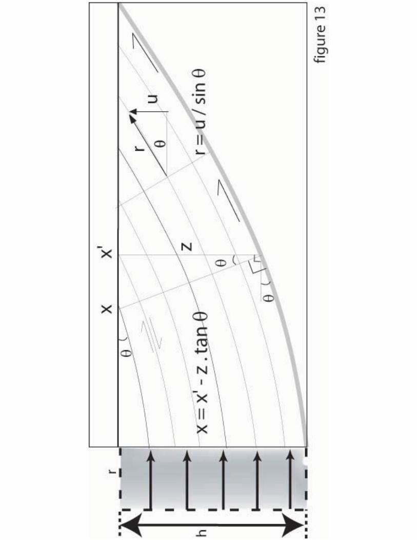
pictured in Figure 13, and hence when the cumulative slip on the ramp exceeds U/sin( ) (where
is the average dip angle of the fault). In the hanging wall, uplift rate depends on the dip of the
fault at depth, which is equal to the local bedding dip angle. If the fault dip angle is at the x’
coordinate, at depth z the x coordinate where the bedding dip angle is is )tan(' zxx
(Figure 13). The relation between the horizontal displacement V(x) and the vertical displacement
U(x) is then simply,
18
19
20
)'(tan)()( xxUxV (10)21
22
23
24
where the fault dip angle (x') at point x’ as defined above. To test the model, the fault shown on
Figure 7C was determined from the measured strain field and adjusted from a fourth order
polynomial. The measurements rather suggest a shear zone with a finite thickness of the order of
16
3 mm. In order to improve the fit of the model and avoid having large misfits near the fault zone
(which could artificially increase the RMS between the data and the predicted displacements),
the predicted displacements were smoothed with a gaussian function with a variance of 3 mm.
We observe that this formulation provides a relatively good fit to the uplift rates, but the
cumulative slip is less than the critical value, U/sin( (RMS of 10.9 10
1
2
3
4
5
6
7
8
9
10
11121314
15
16
17
18
19
20
21
-3 mm/step between steps
150 and 153). If this model were used to estimate shortening rate from the measured uplift rate in
the experiment, it would underestimate the actual value by 8-10 %. This shows that the ramp
overthrusting stage of our experiment does not exactly obey the fault-bend fold model, which
can be explained by the fact that beds near the surface are not yet parallel to the thrust fault at
depth.
5.4 Comparison with a simple shear folding model
Another way to relate horizontal and vertical velocities along the profile after
deformation gets localized is to assume that the hanging wall deforms by simple shear as
pictured in Figure 14. This model obeys mass conservation only if the slip on the fault plane
varies with the fault dip angle. Given that there is no length line change for lines parallel and
perpendicular to the direction of simple shear, the projection of the velocity vector at any point in
the direction perpendicular to the simple shear direction must be constant and equal to r.sin( ),
where r is the shortening at the back of the structure, and the simple shear angle defined in
Figure 14. The slip r’ on the fault is then expressed by :
))(sin(sin)('
x
rxr (11) 22
23 where (x) is the local fault dip angle at point x.
17
The surface uplift at abscissa point x is then related to the uplift on the fault at a point x’
with (Figure 14). The local uplift at the x coordinate can therefore be
written as
1
2
3
tan*)'(' xzxx
4
5
6
)'(sin)'(')( xxrxU , (12)
with (x’) the fault dip angle at point x’, and r’(x’) the slip on the fault at the same point. Using
(11) and (12), we can deduce the shortening r from the uplift profile,
)'(sinsin)'(sin()()(
x
xxUxr . (13)7
8
9
Assuming simple shear deformation, the horizontal displacement V(x) along the section is
then related to the vertical displacement U(x) and the fault dip angle at point x’ according to
))'(tan()()(x
xUxV , (14) 10
11
12
13
14
15
16
17
18
19
20
21
22
where (x’) is the fault dip angle at point x’ as defined above.
This model predicts a sharp discontinuity of displacements across the fault which can
lead to large local misfits when modeled and observed displacements are compared. To
attenuated this effect, the displacements predicted from the model are smoothed with a gaussian
function with a variance of 3 mm.
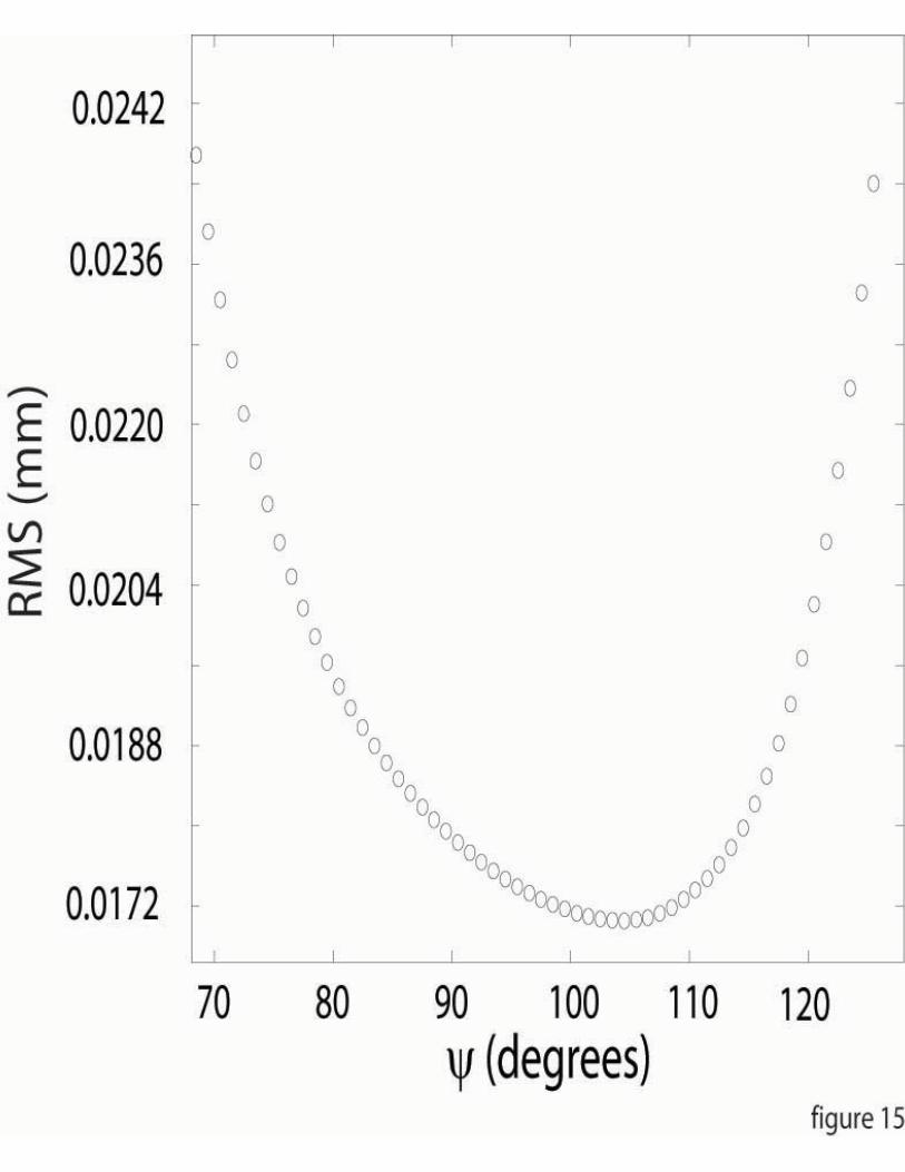
We have next varied the simple shear angle, , in order to maximize the fit to the
observed displacements. It turns out that the best fit is found for an angle of about 105° (Figure
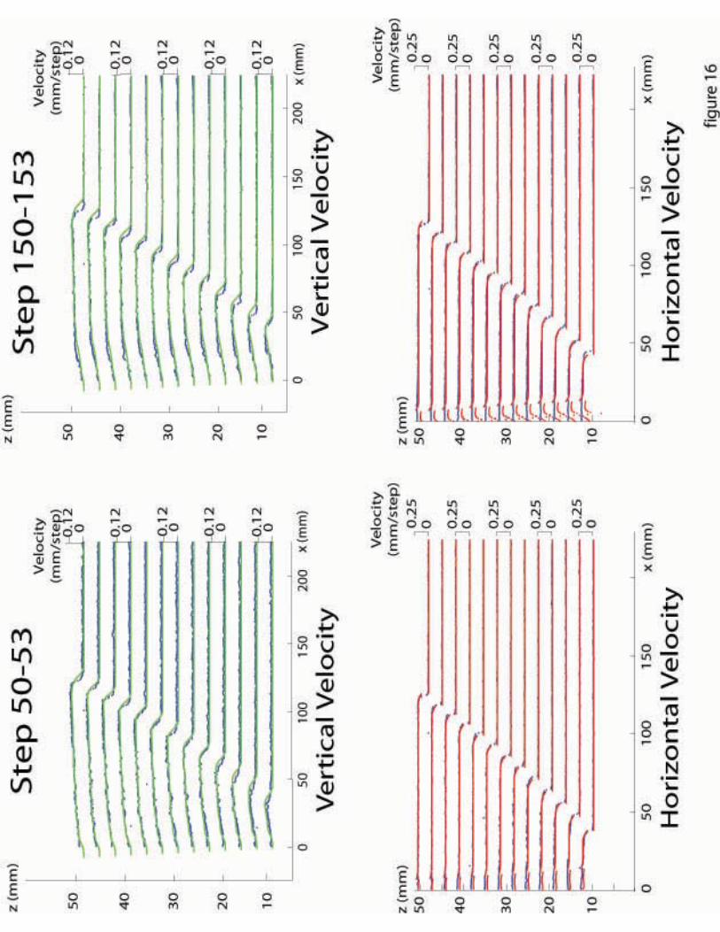
15). This modeling provides an excellent fit to the data (RMS of 8.62 10-3 mm/step for the
vertical velocities and rms of 16.95 10-3mm/step for the horizontal velocities between steps 150
and 153) reconciling both vertical and horizontal velocities (Figure 16), except at the back of the
structure, where the fault is almost horizontal. Because the best fitting shear angle does not
exactly bisect the detachment and the ramp dip angle, this direction of shear implies changes of
18
the thickness and length of the sand layers during folding [Suppe, 1983]. Hanging-wall units
consequently thicken during their transport above the ramp, as also observed in other
experiments [Maillot and Koyi, 2006; Koyi and Maillot, 2006].
1
2
3
4
5
6
7
8
9
10
11
12
13
14
15
16
17
18
19
20
21
22
23
6. Discussion on the folding mechanism observed in the analogue experiment
In this experiment folding results primarily from distributed plastic shear. After a critical
value of shortening (h/8), strain starts to localize and a frontal ramp develops. The ramp forms by
strain localization close to a passive axial surface (the third one described above) where strain
was able to accumulate during the first stage of folding (Figure 17). Because of this location the
tilted forelimb formed earlier becomes part of the footwall once the ramp is formed. Memory of
the initial phase of fault propagation is thus preserved in the footwall and in the hangingwall
from the tilted forelimb. Note that in the presence of erosion, once the system has become a ramp
anticline, the memory of the initial phase of deformation in the hanging wall would be lost but
preserved in the footwall (Figure 17). Such a geometry has been observed across several
piedmont folds north of the Tien Shan which were inferred to have evolved from fault-tip folds
to fault-bend folds [Avouac, et al., 1993].
Qualitatively, the behavior observed in this experiment is probably not specific to the
particular setting of the experiment selected for this study. From a mechanical point of view, the
axial surfaces are the expression of developing conjugate shear bands bounding a symmetrical
pop-up structure (Figure 5B). After the localisation of the favoured fore-thrust shear zone (Figure
5C) back-thrust shear zone is moving as part of the hangingwall on the ramp. The detail of the
kinematics, however, must depend highly on the particular geometrical set-up and material
properties in the selected experiment. For example, it is probable that the amount of distributed
19
1
2
3
4
5
6
7
8
9
10
11
12
13
14
15
16
17
18
19
20
21
22
23
deformation reached before localization is related to the onset of strain hardening and probably
depends on factors such as the grain size and compaction [Lohrmann, et al., 2003]. A complete
mechanical analysis of the observed kinematics is beyond the scope of this study and would
require a parametric study to elucidate the influence of each of the governing material properties
and of the geometry (dependence on layer thickness, dependence on layering, etc.).
During ramp overthrusting, we find a good fit between observed incremental
displacements and the simple-shear model assuming an optimal simple-shear angle of 105º ( in
Figure 14). Most of the shear occurs in the area where the detachment connects with the ramp.
This zone thus appears as a migrating kink band, equivalent to a transient backthrust dipping by
65 º. Maillot and Leroy [2003] have determined the optimal dip of the backthrust in such a fault-
bend fold that would correspond to a minimum of dissipated energy within the whole structure.
The three sources of dissipation are due to frictional sliding on the ramp, on the backthrust and
on the décollement [Maillot and Leroy, 2003]. As mentioned above, the basal coefficient of
friction is estimated to 21° in this experiment. According to Maillot and Leroy [2003], the
optimal dip of the back thrust would be 30° in this case, which implies a simple shear angle of
150° quite different from that observed in the experiment. The system does not seem to respond
as expected from the minimization of total dissipation. The observed kinematics does not
conform either to the kinematics expected from conventional fault-bend folding [Suppe, 1983].
This is because, despite the presence of the glass beads layers, layer-parallel longitudinal strain
dominates over layer-parallel shear in this experiment.
20
7. Guidelines for the analysis of natural fault-tip folds.1
2
3
4
5
6
7
8
9
10
11
12
13
14
15
16
17
18
19
20
21
22
We outline here how the fault-tip fold kinematic model described above can be used to
analyze natural folds. It is first assumed here that cross sectional area is preserved during folding.
It should be recalled that a variety of mechanisms can lead to volume changes in analogue
models, as observed in our experiment, or at the scale of natural folds such as tectonic
compaction, dilatancy, or pressure solution, [Koyi, 1995; Marone, 1998; Whitaker and
Bartholomew, 1999; Lohrmann, et al., 2003; Koyi and Cotton, 2004; Adam, 2005]. The
approach assumes in addition that the deformation field is stationary, meaning that all the axial
surfaces remain fixed relative to the undeformed footwall. This is only a first order
approximation (Figure 7). Provided that these assumptions are correct, the analytic model makes
it possible to retrieve the history of shortening across a fold from growth strata or from deformed
fluvial terraces [Simoes, et al., this issue; Daeron, et al., this issue]. First, the analytical
expressions need to be calibrated based on the finite geometry of the fold, (as images by seismic
profiles for example). As an illustrationand to test the hypothesis that deformation can be
assumed stationnary, we use the finite geometry after 3.4 mm of horizontal shortening, when
localization of the fault has initiated at depth (Figure 18).
7.1 Relating dip-angle and shortening for fault-tip folds.
The key observation in the experiment is that uplift rate varies linearly within domains
Adam, J., J. Urai, B., Wieneke, O. Oncken, K. Pfeiffer, N. Kukowski, J. Lohrmann, S. Hoth, W. van der Zee, and J. Schmatz, J. (2005), Shear localisation and strain distribution during tectonic faulting--new insights from granular-flow experiments and high-resolution optical imagecorrelation techniques, Journal of Structural Geology, 27(2), 283--301.
Allmendinger, R.W. (1998), Inverse and forward numerical modeling of trishear fault-propagation folds, Tectonics 17(4), 640--656.
Allmendinger, R.W. and J.H. Shaw (2000), Estimation of fault propagation distance from fold shape: Implications for earthquake hazard assessment, Geology 28(12), 1099--1102.
Avouac, J. P., P. Tapponier, M. Bai, H. You and G. Wang (1993), Active thrusting and folding along the Northern Tien-Shan and Late Cenozoic Rotation of the Tarim Relative to Dzungaria and Kazakhstan, Journal of Geophysical Research – Solid Earth, 98(B4), 6755—6804.
Brooks, B.A., E. Sandvol, and A. Ross (2000), Fold style inversion: Placing probabilistic constraints on the predicted shape of blind thrust faults, Journal of Geophysical Research – Solid Earth, 105(B6), 13281--13301.
Burbank, D., and R. Anderson (2001) Tectonic geomorphology, p. 274, Blackwell Science, Malden, MA.
Chamberlin, R.T. (1910), ‘The Appalachian folds of central Pennsylvania’, Journal of Geology,27, 228--251.
Chapple, W.M. (1978), Mechanics of thin-skinned fold-and-thrust belts, Geological Society ofAmerica Bulletin, 89(8), 1189--1198.
Daeron, M., J.P. Avouac, J. Charreau, and S. Dominguez, Modeling the shortening history of afault-tip fold using structural and geomorphic records of deformation, Journal of Geophysical Research, this issue.
Dahlstrom, C.D.A. (1990), Geometric constraints derived from the law of conservation ofvolume and applied to evolutionary models for detachment folding, AAPG Bulletin-AmericanAssociation of Petroleum Geologists, 74(3), 336--344.
Davis, D., J. Suppe, and F.A. Dahlen (1983), Mechanics of fold-and-thrust belts and accretionarywedges, Journal of Geophysical Research, 88(NB2), 1153--1172.
Dominguez S., J. Malavieille and S.E. Lallemand (2000). Deformation of margins in response to seamount subduction - insights from sandbox experiments; Tectonics, 19, n°1, 182-196.
Dominguez S., R. Michel, J.P. Avouac, and J. Malavieille (2001). Kinematics of thrust fault propagation, Insight from video processing techniques applied to experimental modeling, EGS XXVI, Nice, March 2001.
Dominguez, S., J. Malavieille, and J.P. Avouac (2003), Fluvial terraces deformation induced by thrust faulting : an experimental approach to better estimate crustal shortening velocities. EGS-AGU-EUG Joint Assembly, Nice, Abstract number EAE03-A-11321
Epard, J.L., and R.H. Groshong (1993), Excess area and depth to detachment, AAPG Bulletin-American Association of Petroleum Geologists, 77(8), 1291--1302.
Epard, J.L., and R.H. Groshong (1995), Kinematic model of detachment folding including limbrotation, fixed hinges and layer-parallel strain, Tectonophysics, 247(1-4), 85--103.
Gutscher, M.A., N. Kukowski, J. Malavieille, and S. Lallemand (1998), Material transfer in accretionary wedges from analysis of a systematic series of analog experiments, Journal of Structural Geology, 20(4), 407--416.
Hardy, S., and J. Poblet (1994), Geometric and numerical-model of progressive limb rotation in detachment folds, Geology, 22(4), 371--374.
Hardy, S., J. Poblet, K. McClay, and D. Waltham (1996), Mathematical modelling of growth strata associated with fault-related fold structures, Special Publication Geological Society, 99,265--282.
Horn, B.K.P., and B.G. Schunck (1980), Determining optical flow, Technical Report A.I. Memo572, Massachusetts Institute of Technology.
Jolivet, M. (2000), Cinématique des déformations au Nord Tibet. Thermochronologie, traces de fission, modélisation analogique et études de terrain, Thesis, Université Montpellier II.
King, G.C.P., R.S. Stein, and J.B. Rundle (1988), The growth of geological structures by repeated earthquakes. 1. Conceptual-framework, Journal of Geophysical Research –Solid Earth and Planets, 93(B11), 13307--13318.
Konstantinovskaia, E., and J. Malavieille (2005), Erosion and exhumation in accretionary orogens: Experimental and geological approaches, Geochemistry Geophysics Geosystems 6,Q02006, doi:10.1029/2004GC000794, ISSN: 1525-2027.
Koyi, H. (1995), Mode of internal deformation in sand wedges, Journal of Structural Geology, 17(2), 293--300.
Koyi H. A., and J. Cotton (2004) Experimental insights on the geometry and kinematics of fold-and-thrust belts above weak, viscous evaporitic decollement; a discussion, Journal of Structural
Koyi, H. and B. Maillot (2006), The effect of ramp dip and friction on thickness change of hangingwall units; a necessary improvement to kinematic models, paper presented at the annual general meeting of the Tectonic Studies Group of the Geological Society of London, Manchester England.
Krantz, R.W. (1991), Measurements of friction coefficients and cohesion for faulting and faultreactivation in laboratory models using sand and sand mixtures, Tectonophysics, 188(1-2), 203--207.
Lohrmann, J., N. Kukowski, J. Adam, and O. Oncken (2003), The impact of analogue materialproperties on the geometry, kinematics, and dynamics of convergent sand wedges, Journal of Structural Geology, 25, 1691--1711.
Lallemand, S.E., P. Schnurle, and J. Malavieille (1994), Coulomb theory applied to accretionaryand nanoaccretionary wedges – Possible causes for tectonic erosion and or frontal accretion, Journal of Geophysical Research – Solid Earth, 99(B6), 12033--12055.
Lavé, J., and J.P. Avouac (2000), Active folding of fluvial terraces across the Siwaliks Hills, Himalayas of central Nepal, Journal of Geophysical Research - Solid Earth, 105(B3), 5735--5770.
Maillot, B., and Y.M. Leroy (2003), Optimal dip based on dissipation of backthrusts and hingesin fold-and-thrust belts, Journal of Geophysical Research, 108 (B6), 2320--2339.
Maillot, B., and H. Koyi (2006), Thrust dip and thrust refraction in fault-bend folds: analogue models and theoretical predictions, Journal of Structural Geology, 28(1), 36--49.
Malavieille, J. (1984). Modélisation expérimentale des chevauchements imbriqués : applicationaux chaînes de montagnes, Bulletin de la Société géologique de France, XXVI(1), 129--138.
Marone, C. (1998), Laboratory-derived friction laws and their application to seismic faulting, Annual Review of Earth and Planetary Sciences, 26, 643—696.
Medwedeff, D.A., and J. Suppe (1997), Multibend fault-bend folding, Journal of Structural Geology, 19(3-4), 279--292.
Mitra, S. (2003), A unified kinematic model for the evolution of detachment folds, Journal of Structural Geology, 25(10), 1659--1673.
Molnar, P., E.T. Brown, B.C. Burchfiel, D. Qidong, F. Xianyue, L. Jun, G.M. Raisbeck, S. Jianbang, W. Zhangming, F. Yiou, and Y. Huichuan (1994), Quaternary climate-change and the formation of river terraces across growing anticlines on the north flank of the Tien-Shan, China, Journal of Geology, 102(5), 583--602.
28
Mosar, J., and J. Suppe (1992), Role of shear in fault-propagation folding., in Thrust tectonics.,edited by K. R. McClay, pp. 123--132, Chapman & Hall, London, United Kingdom (GBR).
Mulugeta, G. (1988), Squeeze Box in a centrifuge, Tectonophysics, 148(3-4), 323--335.
Mulugeta, G., and H. Koyi (1992), Episodic accretion and strain partitioning in a model sand wedge, Tectonophysics, 202(2-4), 319--333
Myers, W. B., and W. Hamilton (1964), Deformation accompanying the Hebgen Lake Earthquake of August 17, 1959, in The Hebgen Lake, Montana, Earthquake of August 17, 1959,U.S. Geol. Surv. Prof. Pap, 435, 55--98.
Okada, Y. (1985), Surface deformation due to shear and tensile faults in a half-space, Bulletin ofthe Seismological Society of America, 75(4), 1135--1154.
Poblet, J., and K. McClay (1996), Geometry and kinematics of single-layer detachment folds, AAPG Bulletin-American Association of Petroleum Geologists, 80(7), 1085--1109.
Press, W. H., S.A. Teukolsky, W.T. Vetterling, and B.P. Flannery, (1995), Numerical Recipes inC: The Art of Scientific Computing (Hardcover), Cambridge University Press.
Rockwell, T.K., E.A. Keller, and G.R. Dembroff (1988), Quaternary rate of folding of the Ventura Avenue anticline, Western Transverse Ranges, Southern California, Geological Society of America Bulletin, 100(6), 850--858.
Savage, H.M., and M.L. Cooke (2004), The effect of non-parallel thrust fault interaction on fold patterns, Journal of Structural Geology, 26(5), 905--917.
Scharer, K.M., D.W. Burbank, J. Chen, R.J. Weldon, C. Rubin, R. Zhao, and J. Shen (2004), Detachment folding in the Southwestern Tian Shan-Tarim foreland, China: shortening estimatesand rates, Journal of Structural Geology, 26(11), 2119--2137.
Schellart, W.P. (2000), Shear test results for cohesion and friction coefficients for different granular materials: scaling implications for their usage in analogue modelling, Tectonophysics,324(1-2), 1--16.
Simoes, M., J.P. Avouac, Y-G. Chen, A.K. Singhvi, C-Y. Wang, M. Jaiswal, Y-C. Chan, and S. Bernard, Kinematic analysis of the Pakuashan fault-tip fold, West Central Taiwan: shorteningrates and age of folding inception, Journal of Geophysical Research-Solid Earth, this issue.
Stein, R.S., G.C.P. King, and J.B Rundle (1988), The growth of geological structures by repeated earthquakes. 2.Fiel examples of continental dip-slip faults, Journal of Geophysical Research - Solid Earth and Planets, 93(B11), 13319--13331.
Storti, F., and J. Poblet (1997), Growth stratal architectures associated to décollement folds and fault-propagation folds. Inferences on fold kinematics, Tectonophysics, 282(1-4), 353--373.
29
123456789
101112131415161718192021222324252627282930313233
34
35
36
37
38
39
Suppe, J. (1983), Geometry and kinematics of fault-bend folding, American Journal of Science, 283(7), 684--721.
Suppe, J., and D.A. Medwedeff (1990), Geometry and kinematics of fault-propagation folding, Eclogae Geologicae Helvetiae, 83(3), 409--454.
Suppe, J., G.T. Chou, and S.C. Hook (1992), Rates of folding and faulting determined from growth strata, in Thrust Tectonics, edited by K. R. McClay, pp. 105--121, Chapman and Hall, New York.
Thompson, S.C., R.J. Weldon, C.M. Rubin, K. Abdrakhmatov, P. Molnar, and G.W. Berger (2002), Late Quaternary slip rates across the central Tien Shan, Kyrgyzstan, central Asia, Journal of Geophysical Research - Solid Earth, 107(B9), 2203.
Van der Woerd, J., X.W. Xu, H.B. Li, P. Tapponnier, B. Meyer, F.J. Ryerson, A.S. Meriaux, and Z.Q. Xu (2001), Rapid active thrusting along the northwestern range front of the Tanghe Nan Shan (western Gansu, China), Journal of Geophysical Research - Solid Earth, 106(B12), 30475--30504.
Ward, S.N., and G. Valensise (1994), The paleo-verdes terraces, California – Bathtub rings from a buried reverse-fault, Journal of Geophysical Research - Solid Earth, 99(B3), 4485--4494.
Whitaker, A. E., and M. J. Bartholomew (1999), Layer parallel shortening: A mechanism for determining deformation timing at the junction of the central and southern Appalachians, American Journal of Science, 299(3), 238-254.
Wickham, J. (1995), Fault displacement-gradient folds and the structure at Lost-Hills, California (USA), Journal of Structural Geology, 17(9), 1293--1302.
Zehnder, A.T., and R.W. Allmendinger (2000), Velocity field for the Trishear model, Journal of Structural Geology, 22(8), 1009--1014.
Table
Table 1 : List and definition of the variables introduced in the analysis.
Figure captions
30
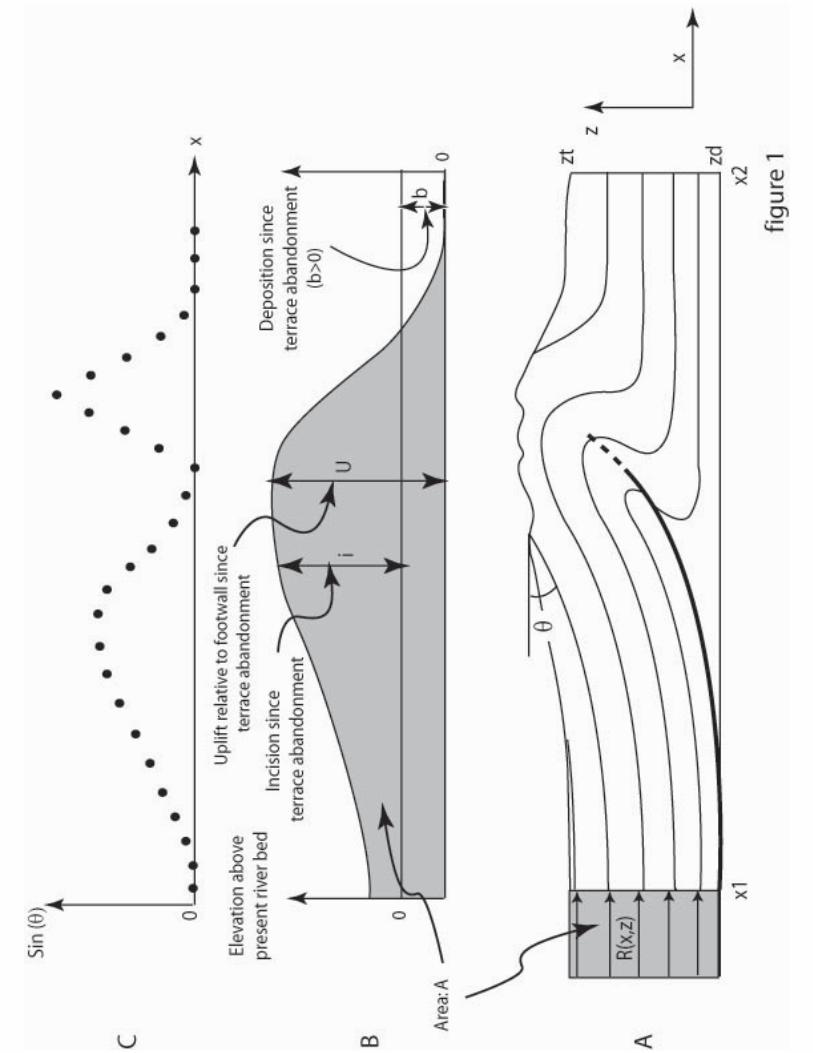
Figure 1: A. Structure of a mature fault-tip fold. B. Continuous profile of a deformed terrace
across the fold can be used to measure incremental folding. The area A defined by the deformed
terrace above its initial geometry may be related to the total displaced area at the back of the fold
since the terrace was abandoned (A) C. Sine of bedding dip angle along structural section, as for
use in equation (1). It might be appropriate to perform such analysis to retrieve incremental
deformation within the backlimb of the fault-tip fold represented, since it appears to be more
mature in this portion of the fold, but may lead to large errors at the front where the structure is
not mature enough and appears more complex.
1
2
3
4
5
6
7
8
9
10
11
12
13
14
15
16
17
18
19
20
21
22
23
Figure 2: Classification of fold models with emphasis on the kinematic record provided by the
architecture of growth strata [Burbank and Anderson, 2001]. A- fault-bend folding [Suppe, 1983;
Medwedeff and Suppe, 1997] results from the transfer of slip from a deeper to a shallower
stratigraphic detachment level. The model assumes conservation of bed thickness and length
during deformation. The hanging wall deforms by bed-parallel simple shear and axial surface
migration. This model applies to mature faults, with a cumulative slip larger than the distance
from the décollement to the surface (measured along the fault). B Various possible geometries of
folds formed at the tip of a blind thrust fault. The fault-propagation fold model (B1) assumes
conservation of bed length and thickness [Suppe and Medwedeff, 1990; Mosar and Suppe, 1992].
The slip gradient model (B2) does not require fault propagation. It assumes conservation of area
but not of bed length [Wickham, 1995]. Model B3 assumes a changing bed length and forelimb
angle [Dahlstrom, 1990; Epard and Groshong, 1995; Mitra, 2003]. Model B4 assumes a
triangular shaped zone of distributed shear [Erslev, 1991; Allmendinger, 1998]. The choice of
the appropriate model to use in the analysis of a natural case example is not straightforward.
31
1
2
3
4
5
6
7
8
9
10
11
12
13
14
15
16
17
18
19
20
21
22
23
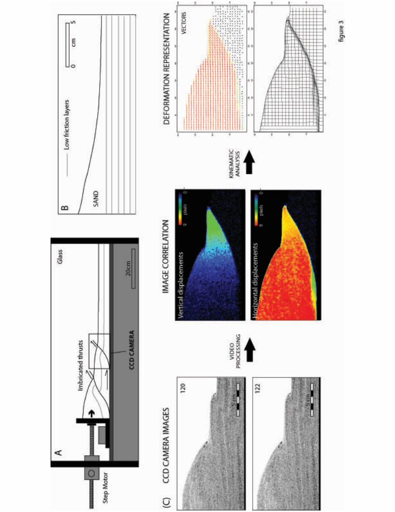
Figure 3: (A) Experimental set-up. To build the model, granular materials were sprinkled into a
20 cm wide and 100 cm long box equipped with transparent side walls, similar to the
experimental set-up used by Dominguez et al. [2000]. The sand layers slide on a horizontal ( =0)
basal polyvinyl chloride (PVC) plate, 2 cm thick. Initially undeformed sand mass is compressed
and deformed by a backstop moved by a step motor. A CCD camera takes pictures (6.3 Mpixels
with a spatial resolution of 0.04 m2) with a constant time step corresponding to 0.2 mm
(equivalent to 2.7 pixel) of shortening between two successive images. (B) Initial conditions.
Five low frictions glass bead layers are interlayered with the sand layers. (C) Summary of the
optical flow technique for measuring displacements. The numerical video image at step 122 is
compared to the one at step 120. The displacement field is computed from the optical flow
technique as described in the text. The incremental displacement field is represented by vectors
or a deformed grid. Also shown is the second invariant of the strain tensor (I2 = 1/2[tr( )2-tr( 2)]
where is the deformation tensor), in gray scale to emphasize zones of strain localization
Figure 4: Incremental displacement field and strain measured during the stage of detachment-tip
folding (between steps 05 and 08, cumulative shortening = 1 mm), the transitional stage of strain
localization (between steps 20 and 23, cumulative shortening = 4.2 mm), and the stage of ramp
overthrusting (between steps 80 and 83, cumulative shortening = 17 mm and between steps 200
and 203, cumulative shortening = 42.6 mm). For each of these plots the cumulative horizontal
shortening is indicated. Note that in the early stage, deformation is not localized. After a
cumulative shortening of about 6 mm it localizes on a frontal ramp connecting the basal
décollement with the surface.
32
1
2
3
4
5
6
7
8
9
10
11
12
13
14
15
16
17
18
19
20
21
22
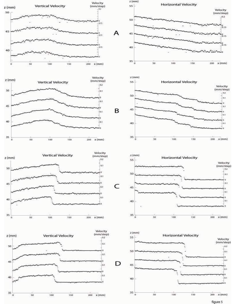
Figure 5: Horizontal and vertical displacement rates measured along profiles run at different
depths during (A) the detachment-tip folding stage (between steps 10 and 12, cumulative
shortening = 2.1 mm), (B) the transitional stage of strain localization (between steps 20 and 23,
cumulative shortening = 4.2 mm) and (C and D) the stage of ramp overthrusting between steps
50 and 53 (cumulative shortening = 10.6 mm) and between steps 150 and 153 (cumulative
shortening = 32 mm). The abscissa axis is positioned at the depth at which each profile is run.
Figure 6: Uplift rates during the detachment-tip folding stage (between steps 10 and 12),
measured along profiles at different depths. For each profile, the position of the ordinate axis
indicates the depth at which the profile is examined. The position of the various axial surfaces
determined from the break-in-slope (circles) is indicated, as well as the locus of the maximum
uplift rate on each profile (dark line). The first, second and third axial surfaces are reasonably
well fit by a straight line suggesting a linear dependency with depth. A straight line also fits
reasonably well the abscissa corresponding to the maximum uplift rates on each profile. The
most frontal axial surface can be adjusted with a second order polynomial.
Figure 7: (A) Schematic pattern of uplift rates and horizontal velocities at various depths. As
deformation increases, the positions of the axial surfaces evolve, in particular axial surfaces 3
and 4 nearly coalesce to define a localized shear zone corresponding to the frontal ramp. (B)
Location of the three frontal axial surfaces during the experiment. (C) Geometry of the frontal
33
1
2
3
4
5
6
7
fault which forms after about 6 mm of shortening together with the positions of the axial surfaces
determined from the vertical displacements.
Figure 8: Maximum uplift rate (at z = 50 mm) as a function of cumulative shortening. In the
early stage of the experiment, during the stage of detachment-tip folding and the transitional
stage of strain localization, before deformation gets strongly localized, the maximum uplift rate
increases gradually. Once deformation is localized on a frontal ramp the maximum uplift rate is
independent of the cumulative shortening and is simply maxmax rU sin* where r is the
shortening rate and
8
9
10
11
12
13
14
15
16
17
18
19
20
21
22
23
max is the maximum dip angle of the fault, about 25°.
Figure 9: (A) Maximum uplift rates as a function of elevation above the décollement during the
stage of detachment-tip folding (values from steps 10-12). A linear function (dashed line), as
proposed in equation (5), provides a good fit (B) Normalized uplift rates at several depths. Uplift
rates are normalized by the value of the maximum at each depth (values from steps 10-12).
Figure 10: Comparison of the measured displacements (blue dots) before fault localization
during the detachment-tip folding stage (between steps 10 and 12) (A), and transitional stage of
strain localization (between steps 20 and 23) (B) (ie for a cumulative shortening lower than 6
mm), and those predicted from the linear model detailed in text (red or green continuous lines).
The rms of the fit to the uplift rate is 0.012103 mm/step between steps 10 and 12 (computed for
the profile at an elevation of 50 mm above the décollement). The fit to the horizontal velocities
yields a rms of 0.021771 mm/step between steps 10 and 12.
34
Figure 11: Results from dislocation modeling of observed vertical and horizontal velocities
during the stage of detachment-tip folding, phase of fault-tip folding (between steps 10 and 12),
using the theory of a dislocation in a elastic half space [Okada, 1985]. (Top left) Measured (blue)
and modeled (black) vertical displacement at the surface. (Top right) Horizontal displacements
extracted from the data (red) and calculated (lack). (Bottom left) Shape of the fault used to
calculate displacement. (Bottom right) Value of the root mean square difference between
observed and calculated vertical displacement as a function of slip rate on the décollement.
1
2
3
4
5
6
7
8
9
10
11
12
13
14
15
16
17
18
19
20
21
22
23
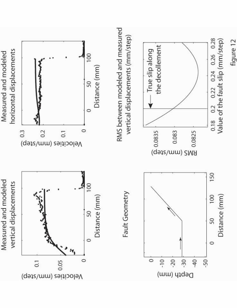
Figure 12: Results from dislocation modeling of observed vertical and horizontal velocities
during the stage of ramp overthrusting (between steps 150 and 153). (Top left) Vertical
displacement at the surface extracted from the data (blue) and calculated (black). (Top right)
Horizontal displacements extracted from the data (red) and calculated (black). (Bottom left)
Shape of the fault used to calculate displacement. (Bottom right) Value of the square difference
between observed and calculated vertical displacement vs the fault slip.
Figure 13: Diagram showing how the incremental uplift, u, of an initially horizontal horizon
relates to incremental shortening in the case of a mature fault-bend fold. The model assumes
conservation of bed thickness and bed length and the hanging wall deforms only by bed-parallel
shear. Uplift is proportional to the sine of the fault dip angle, equivalent to the local bedding dip
angle, , and to the slip along the fault (equation (1)). The assumption of a constant bed
thickness and length during deformation requires that at point with abscissa x at the surface the
bedding dip angle equals the fault dip angle at the point with abscissa x’ along the fault.
35
Figure 14: Sketch showing the relation between incremental shortening r and uplift of an
initially horizontal horizon in the case of a ramp anticline with simple shear deformation of the
hanging wall (simple shear angle ). Conservation of area implies that slip has to vary along the
fault.
1
2
3
4
5
6
7
8
9
10
11
12
13
14
15
16
17
18
19
20
21
22
23
Figure 15: Plot showing how a model of ramp overthrusting with simple shear deformation of
the hanging wall fits the observed uplift rates when the simple shear angle is varied (see sketch
Figure 14). The best fitting shear angle is 104°. This result holds for all incremental
displacements during this kinematic stage.
Figure 16: Comparison between observed horizontal and vertical velocities (blue dots) and the
theoretical profiles (red or green continuous lines) predicted from ramp overthrusting with
simple shear deformation of the hanging wall for a shear angle of 105º as sketched in Figure 15.
See text for details.
Figure 17: Finite deformation of layers initially horizontal computed from the proposed
analytical approximation to the measured displacement fields. Horizontal and vertical
displacements are exaggerated by a factor of 8 for readability. At each stage the cross-section is
obtained by applying incremental deformation to the previous stage. Erosion is not simulated,
but displacements above the deformed surface after the first incremental shortening (0.2 mm)
have not been modeled. The first 2 mm of shortening are not taken into account in this modeling.
This choice implies a fault initiation after only 4 mm of shortening instead of 6 mm as discussed
36
1
2
3
4
5
6
7
8
9
10
11
12
13
14
15
16
17
18
19
20
21
22
23
in the text. The phase of fault-tip folding, up to 2.125 mm of shortening, assumes a stationary
velocity field equivalent to that defined from steps 10 to 12 in the experiment. This corresponds
to the phase of fault-tip folding. The fold structure for a shortening of 2.75 and 3.4 mm,
corresponding to the transitional stage of strain localization, was obtained from the velocity
fields derived from steps 20 to 23 at the onset of strain localization within the sand layers. Above
4 mm of shortening we assume ramp overthrusting with simple shear deformation of the hanging
wall as observed in the experiment from steps 50 to 53 (stage of ramp overthrusting).
Figure 18: Structure of the modeled fold after an actual shortening of 3.4 mm corresponding to
Figure 17. The geometry of the fold is not exaggerated here. The backlimb has been extrapolated
slightly outside the zone covered by our measurements. Each colored surface corresponds to the
fold core area (or ‘excess area’) above the initial elevation of the considered strata. Inclined lines
indicate axial surfaces delimiting domains of homogeneous finite dips as determined from this
finite structure.
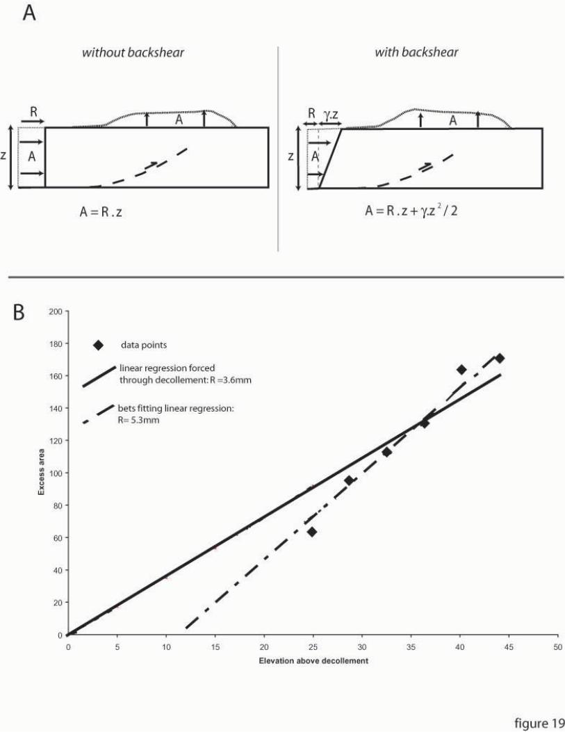
Figure 19: Excess-area as a function of elevation above the décollement.(A) In the absence of
any backshear excess area, A, varies linearly with elevation above the décollement following
Chamberlin’s law [Chamberlin, 1910]. In case of backshear the relationship is no more linear.
(B) Variations of excess area, as derived from Figure 18, as a function of elevation. A simple
linear regression through the data yields a finite shortening of 5.3 mm too high, and a
décollement level too shallow. If the regression is forced through the origin to account for the
known décollement, the estimated total shortening is close to the real value of 3.4 mm.
37
1
2
3
4
5
6
7
8
9
10
11
12
13
14
15
16
17
18
19
Figure 20: Parameters of the analytical formulations derived from the finite structure of the
synthetic fold.(a) as a function of depth. (b) i for each one of the three domains
Figure 21: Computing the misfits between the observed the modeled fold kinematics. Residuals
correspond to predicted minus observed dips or displacements. A- Distribution of the computed
residuals in the dip angles between predicted and observed finite structures. Standard deviation
and median are also reported. The highest residuals are observed in the vicinity of the axial
surface lines. B- Residuals between predicted and observed horizontal incremental displacements
for a total incremental displacement of 1mm at the back of the system. Most of the misfits occur
around the shear bands that develop essentially at the front of the fold during steps corresponding
to a cumulative shortening of 2.75 mm and 3.4 mm of Figure 18. Except for this area where
deformation is underestimated by the model, the predicted horizontal displacements are in good
agreement with the observed ones, within 10% of the applied displacement at the back of the
system C- Residuals between predicted and observed vertical incremental displacements for a
total incremental displacement of 1mm at the back of the system. Most of the underestimation of
vertical incremental deformation results also from the influence of the shear bands at the front of
the fold. As previously, the model is able to predict correctly the incremental displacements
within 10% of the shortening applied at the back of the system.


![KINEMATICS - new.excellencia.co.innew.excellencia.co.in/college/web/pdf/Kinematics-merged.pdf · KINEMATICS KINEMATICS WORKSHEET 1 1) Displacement is a _____ [ ] 1) Vector quantity](https://static.documents.pub/doc/80x56/5f356d4687229051801abace/kinematics-new-kinematics-kinematics-worksheet-1-1-displacement-is-a-.jpg)


