+ All Categories
Home > Documents > 1 Layered Downlink Precoding for C-RAN Systems with Full ... · PDF file1 Layered Downlink...

1 Layered Downlink Precoding for C-RAN Systems with Full ... · PDF file1 Layered Downlink...

Date post: 15-Feb-2018
Category:
Upload: vutuong
View: 218 times
Download: 0 times
Share this document with a friend
29
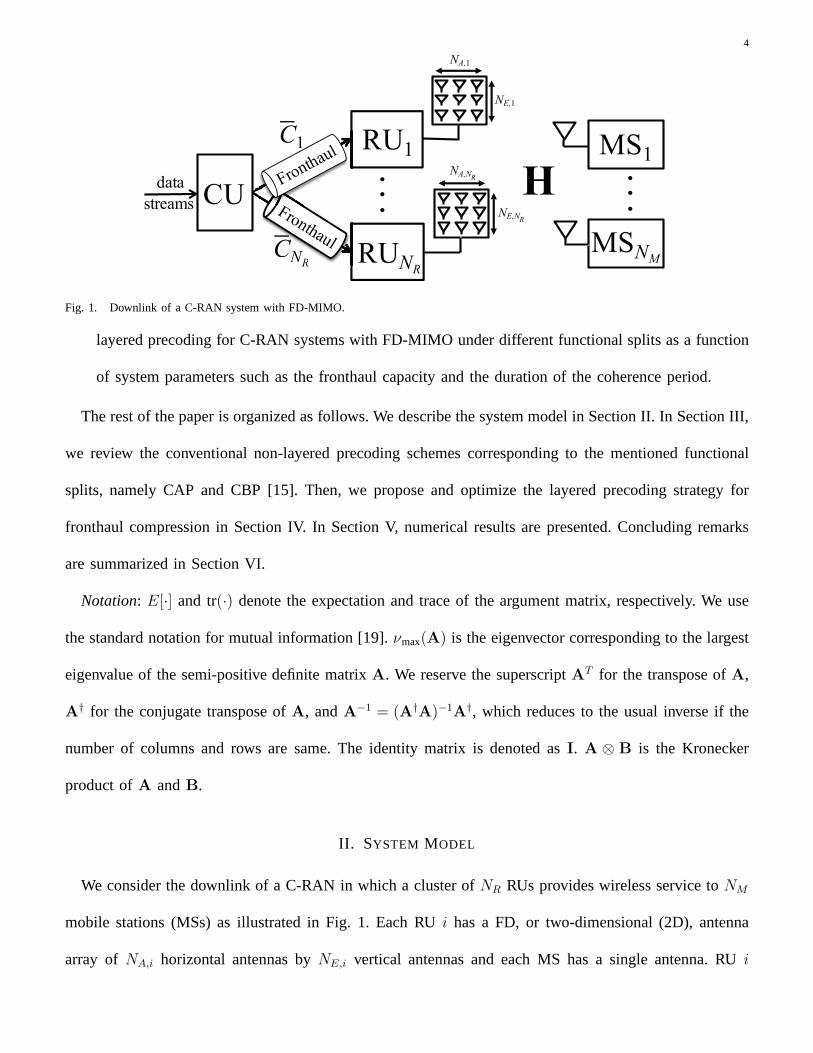
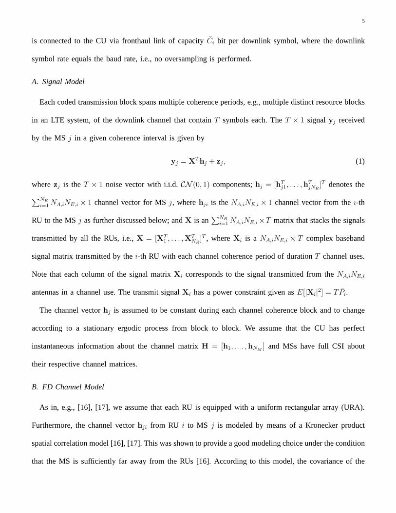
arXiv:1511.08084v1 [cs.IT] 25 Nov 2015 1 Layered Downlink Precoding for C-RAN Systems with Full Dimensional MIMO Jinkyu Kang, Osvaldo Simeone, Joonhyuk Kang and Shlomo Shamai (Shitz) Abstract The implementation of a Cloud Radio Access Network (C-RAN) with Full Dimensional (FD)-MIMO is faced with the challenge of controlling the fronthaul overhead for the transmission of baseband signals as the number of horizontal and vertical antennas grows larger. This work proposes to leverage the special low-rank structure of FD-MIMO channel, which is characterized by a time-invariant elevation component and a time-varying azimuth component, by means of a layered precoding approach, so as to reduce the fronthaul overhead. According to this scheme, separate precoding matrices are applied for the azimuth and elevation channel components, with different rates of adaptation to the channel variations and correspondingly different impacts on the fronthaul capacity. Moreover, we consider two different Central Unit (CU) - Radio Unit (RU) functional splits at the physical layer, namely the conventional C-RAN implementation and an alternative one in which coding and precoding are performed at the RUs. Via numerical results, it is shown that the layered schemes significantly outperform conventional non-layered schemes, especially in the regime of low fronthaul capacity and large number of vertical antennas. Index Terms Cloud-Radio Access Networks (C-RAN), Full Dimensional (FD)-MIMO, fronthaul compression, layered pre- coding. Jinkyu Kang and Joonhyuk Kang are with the Department of Electrical Engineering, Korea Advanced Institute of Science and Technology (KAIST) Daejeon, South Korea (Email: [email protected] and [email protected]). O. Simeone is with the Center for Wireless Communications and Signal Processing Research (CWCSPR), ECE Department, New Jersey Institute of Technology (NJIT), Newark, NJ 07102, USA (Email: [email protected]). S. Shamai (Shitz) is with the Department of Electrical Engineering, Technion, Haifa, 32000, Israel (Email: [email protected]).
Transcript

arX

iv:1

511.

0808

4v1

[cs.

IT]

25 N

ov 2

015

1

Layered Downlink Precoding for C-RAN Systems

with Full Dimensional MIMO

Jinkyu Kang, Osvaldo Simeone, Joonhyuk Kang and Shlomo Shamai (Shitz)

Abstract

The implementation of a Cloud Radio Access Network (C-RAN) with Full Dimensional (FD)-MIMO is faced

with the challenge of controlling the fronthaul overhead for the transmission of baseband signals as the number

of horizontal and vertical antennas grows larger. This workproposes to leverage the special low-rank structure of

FD-MIMO channel, which is characterized by a time-invariant elevation component and a time-varying azimuth

component, by means of a layered precoding approach, so as toreduce the fronthaul overhead. According to

this scheme, separate precoding matrices are applied for the azimuth and elevation channel components, with

different rates of adaptation to the channel variations andcorrespondingly different impacts on the fronthaul

capacity. Moreover, we consider two different Central Unit(CU) - Radio Unit (RU) functional splits at the physical

layer, namely the conventional C-RAN implementation and analternative one in which coding and precoding

are performed at the RUs. Via numerical results, it is shown that the layered schemes significantly outperform

conventional non-layered schemes, especially in the regime of low fronthaul capacity and large number of vertical

antennas.

Index Terms

Cloud-Radio Access Networks (C-RAN), Full Dimensional (FD)-MIMO, fronthaul compression, layered pre-

coding.

Jinkyu Kang and Joonhyuk Kang are with the Department of Electrical Engineering, Korea Advanced Institute of Science and Technology

(KAIST) Daejeon, South Korea (Email: [email protected] and [email protected]).

O. Simeone is with the Center for Wireless Communications and Signal Processing Research (CWCSPR), ECE Department, NewJersey

Institute of Technology (NJIT), Newark, NJ 07102, USA (Email: [email protected]).

S. Shamai (Shitz) is with the Department of Electrical Engineering, Technion, Haifa, 32000, Israel (Email: [email protected]).

2

I. INTRODUCTION

The cloud radio access network (C-RAN) architecture consists of multiple radio units (RUs) connected

via fronthaul links to a central unit (CU) that implements the protocol stack of the RUs, including baseband

processing [1], [2]. C-RAN enables a significant reduction in capital and operating expenses, as well as

an enhanced spectral efficiency by means of joint interference management at the physical layer across

all connected RUs. Nevertheless, it is well recognized thatthe performance of this architecture is limited

by the capacity and latency constraints of the fronthaul network connecting RUs and CU [1]–[4].

In a standard C-RAN implementation, the fronthaul links carry digitized baseband signals. Hence, the bit

rate required for a fronthaul link is determined by the quantization and compression operations applied to

the baseband signals prior to transmission on the fronthaullinks. As such, the fronthaul rate is proportional

to the signal bandwidth, to the oversampling factor, to the resolution of the quantizer/compressor, and to

the number of antennas [5]. The fronthaul bit rate can be reduced by implementing alternative functional

splits between CU and RU, whereby some baseband functionalities are implemented at the RU [6]–[8].

As a concurrent trend in the evolution of wireless networks,in the 3rd generation partnership project

(3GPP) long term evolution (LTE) Release-13, three-dimensional (3D)-MIMO, where base stations are

equipped with two-dimensional rectangular antenna arrays, has been intensely discussed as a promising

tool to boost spectral efficiency [9], [10]. 3D-MIMO technology is classified into three categories, namely,

vertical sectorization (VS), elevation beamforming (EB),and Full-Dimensional MIMO (FD-MIMO) in

order of complexity. The VS scheme splits a sector of cellular coverage into multiple sectors by means of

different electrical downtilt angles. With the EB approach, instead, users are supported by predetermined or

adaptive beams in the elevation direction. Finally, in FD-MIMO, the spatial diversity provided by vertical

and horizontal antennas is leveraged jointly to serve multiple users using multiuser-MIMO techniques.

Endowing RUs with two-dimensional arrays in a C-RAN system (see Fig. 1), while promising from a

spectral efficiency perspective, creates significant challenges in terms of fronthaul overhead as the number

of antennas grows larger [11]. In this paper, we focus on the design of downlink precoding for C-RANs

3

with FD-MIMO RUs by accounting for the impact of fronthaul capacity limitations. Previous works [4],

[12]–[15] on precoding design for the downlink of C-RAN systems either assume fixed channel matrices

with full channel state information (CSI), see [4], [12]–[14], or considers ergodic channels with generic

correlation structure and possibly imperfect CSI [15]. Importantly, these works do not account for the

special features of FD channel models [16], [17] and hence donot bring insights into the feasibility of

a C-RAN deployment based on FD-MIMO. In particular, the FD-MIMO channel is understood to be

characterized by time variability at different time scalesfor elevation and azimuth components; elevation

component changes significantly more slowly than the rate ofchange of the more conventional azimuth

component [16].

In order to address the design and performance of C-RAN system with FD-MIMO, this paper puts

forth the following contributions.

• A layered precoding scheme is proposed whereby separate precoding matrices areapplied for the

azimuth and elevation channel components with a different rate of adaptation to the channel variations.

Specifically, a single precoding matrix is designed for the elevation channel across all coherence times

based on stochastic CSI, while precoding matrices are optimized for the azimuth channel by adapting

instantaneous CSI. This layered approach, considered in [17] for a conventional cellular architecture,

has the unique advantage in a C-RAN of potentially reducing the fronthaul transmission rate, due to

the opportunity to amortize the overhead related to the elevation channel component across multiple

coherence times.

• We study layered precoding in a C-RAN system by considering two different CU-RU functional splits

at the physical layer, namely the conventional C-RAN implementation, referred to as Compress-After-

Precoding (CAP) as in [4], [12]–[15], whereby all baseband processing is done at the CU, and an

alternative split, known as Compress-Before-Precoding (CBP) [15], [18], in which channel encoding

and precoding are instead performed at the RUs.

• We carry out a performance comparison between standard non-layered precoding strategies and

4

.

.

.H

.

.

.

MSNM

MS1RU1

RUNR

CU

NE,1

NA,1

NE,NR

NA,NR

C!NR

data

streams

C!NC RN

C!1C1

Fig. 1. Downlink of a C-RAN system with FD-MIMO.

layered precoding for C-RAN systems with FD-MIMO under different functional splits as a function

of system parameters such as the fronthaul capacity and the duration of the coherence period.

The rest of the paper is organized as follows. We describe thesystem model in Section II. In Section III,

we review the conventional non-layered precoding schemes corresponding to the mentioned functional

splits, namely CAP and CBP [15]. Then, we propose and optimize the layered precoding strategy for

fronthaul compression in Section IV. In Section V, numerical results are presented. Concluding remarks

are summarized in Section VI.

Notation: E[·] and tr(·) denote the expectation and trace of the argument matrix, respectively. We use

the standard notation for mutual information [19].νmax(A) is the eigenvector corresponding to the largest

eigenvalue of the semi-positive definite matrixA. We reserve the superscriptAT for the transpose ofA,

A† for the conjugate transpose ofA, andA−1 = (A†A)−1A†, which reduces to the usual inverse if the

number of columns and rows are same. The identity matrix is denoted asI. A ⊗ B is the Kronecker

product ofA andB.

II. SYSTEM MODEL

We consider the downlink of a C-RAN in which a cluster ofNR RUs provides wireless service toNM

mobile stations (MSs) as illustrated in Fig. 1. Each RUi has a FD, or two-dimensional (2D), antenna

array of NA,i horizontal antennas byNE,i vertical antennas and each MS has a single antenna. RUi

5

is connected to the CU via fronthaul link of capacityCi bit per downlink symbol, where the downlink

symbol rate equals the baud rate, i.e., no oversampling is performed.

A. Signal Model

Each coded transmission block spans multiple coherence periods, e.g., multiple distinct resource blocks

in an LTE system, of the downlink channel that containT symbols each. TheT × 1 signalyj received

by the MSj in a given coherence interval is given by

yj = XThj + zj, (1)

wherezj is theT × 1 noise vector with i.i.d.CN (0, 1) components;hj = [hTj1, . . . ,h

TjNR

]T denotes the

∑NR

i=1NA,iNE,i × 1 channel vector for MSj, wherehji is theNA,iNE,i × 1 channel vector from thei-th

RU to the MSj as further discussed below; andX is an∑NR

i=1NA,iNE,i×T matrix that stacks the signals

transmitted by all the RUs, i.e.,X = [XT1 , . . . ,X

TNR

]T , whereXi is a NA,iNE,i × T complex baseband

signal matrix transmitted by thei-th RU with each channel coherence period of durationT channel uses.

Note that each column of the signal matrixXi corresponds to the signal transmitted from theNA,iNE,i

antennas in a channel use. The transmit signalXi has a power constraint given asE[|Xi|2] = T Pi.

The channel vectorhj is assumed to be constant during each channel coherence block and to change

according to a stationary ergodic process from block to block. We assume that the CU has perfect

instantaneous information about the channel matrixH = [h1, . . . ,hNM] and MSs have full CSI about

their respective channel matrices.

B. FD Channel Model

As in, e.g., [16], [17], we assume that each RU is equipped with a uniform rectangular array (URA).

Furthermore, the channel vectorhji from RU i to MS j is modeled by means of a Kronecker product

spatial correlation model [16], [17]. This was shown to provide a good modeling choice under the condition

that the MS is sufficiently far away from the RUs [16]. According to this model, the covariance of the

6

!"#$(1)

%

!"#$(2) !"#

$(3) !"#$(t). . .

&"#'

Fig. 2. Illustration of time variability of the azimuth component{hAji(t)} and of the elevation componentuE

ji in the FD channel model

(3). The notationhAji(t) emphasizes the dependence on the coherence blockt of the azimuth component of the channel.

3D channelhji which is defined asRji = E[hjih†ji], is written as

Rji = RAji ⊗RE

ji, (2)

whereRAji andRE

ji represent the covariance matrices in the azimuth and elevation directions, respectively.

Since the elevation direction is typically subject to negligible scattering [20], [21], the elevation covariance

matrix REji may be assumed to be a rank-1 matrix, i.e.,RE

ji = uEjiu

E †ji , whereuE

ji is aNE,i× 1 unit-norm

vector [17]. Under this assumption, the channel vectorhji can be written as

hji =√αjih

Aji ⊗ uE

ji, (3)

whereαji denotes the path loss coefficient between MSj and RUi as

αji =1

1 +(

djid0

)η , (4)

with dji being the distance between thej-th MS and thei-th RU, d0 being a reference distance, andη

being the path loss exponent; andhAji ∼ CN (0,RA

ji) with RAji having diagonal elements equal to one.

This model entails that the elevation componentshEji remains constant over coherence interval, while the

azimuth component changes independent across coherence interval ashAji ∼ CN (0,RA

ji), as illustrated in

Fig. 2.

III. B ACKGROUND

In this section, we briefly recall in an informal fashion two baseline strategies for downlink transmission

in the C-RAN system introduced above. The strategies correspond to two different functional splits at

the physical layer between CU and RUs [5], [6] as detailed in [15]. We note that these schemes were

7

Channel

coding

Channel

coding

.

.

.Precoding

Precoding

design

CSI

Q...

CU

RU1

RUNR

.

.

.

.

.

.

S1

SNM

!"1

!"NR

Wdata

streamsFronthaul

FronthaulQ

!#

!NR

Fig. 3. Block diagram of the (non-layered) Compression-After-Precoding (CAP) scheme (“Q” represents fronthaul compression).

previously proposed and studied without specific referenceto FD-MIMO and hence do not leverage the

special structure of the channel model (3).

A. Standard C-RAN Processing: Precoding at the CU

In the standard C-RAN approach, all baseband processing is done at the CU. Specifically, as illustrated in

Fig. 3, the CU performs channel coding and precoding, and then compresses the resulting baseband signals

so that they can be forwarded on the fronthaul links to the corresponding RUs. The RUs upconvert the

received quantized baseband signal prior to transmission on the wireless channel. Following [15], we refer

to this strategy as Compression-After-Precoding (CAP). Analysis and optimization of the CAP strategy

can be found in [15].

B. Alternative Functional Split: Precoding at the RUs

As an alternative to the standard C-RAN approach just described, one can instead implement channel

encoding and precoding at the RUs. This is referred to as Compression-Before-Precoding (CBP) in [15],

[18]. According to this solution, as seen in Fig. 4, the CU calculates the precoding matrices based on the

available CSI, but does not perform precoding. Instead, it uses the fronthaul links to communicate the

downlink information streams to each RU, along with the compressed precoding matrix. Each RU can then

encode and precode the messages of the MSs based on the information received from the fronthaul link.

As elaborated on in [15], this alternative functional splitis generally advantageous when the number of

MSs is not too large and when the coherence periodT is large enough. This is because, when the number

8

Precoding

design

CSIMUX

.

.

.

CU

MUX

Q

Q

.

.

.

De-

MUX

De-

MUX

Q-1Pre-

coding

Pre-

coding

RU1

RUNR

!1

"

!NR

"

!#NR

"

!#1

"

data

streams

Cluster-

ing

Fronthaul

Fronthaul

Channel

coding

Q-1

Channel

coding

$%

$NR

Fig. 4. Block diagram of the (non-layered) Compression-Before-Precoding (CBP) scheme (“Q” represents fronthaul compression).

of MSs is small, a lower fronthaul overhead is needed to communicate the data streams of the MSs on

the fronthaul link; and, when the coherence periodT is large, the compressed precoding information can

be amortized over a longer period, hence reducing the fronthaul rate.

IV. L AYERED PRECODING FORREDUCED FRONTHAUL OVERHEAD

The baseline state-of-the-art fronthaul transmission strategies mentioned above do not make any pro-

vision to exploit the special structure of the FD channel model (3), and can hence be inefficient if the

number of vertical antennas is large. In this section, we propose a layered precoding that instead leverages

the different dynamic characteristic of the elevation and azimuth channels as per channel model (3). We

recall that, according to this model, the elevation channelhas a constant direction across the coherence

periods in its elevation component due to the rank-1 covariance matrix, while its azimuth component

changes in each coherence period due to the generally largerrank of its covariance matrix (see Fig. 2).

In order to exploit this channel decomposition, we propose that the CU designs separate precoding

matrices for the elevation and azimuth channels following alayered precoding approach. The key idea is

that of designing a single precoding matrix for the elevation channel across all coherence times based on

long-term CSI, while adapting only the azimuth precoding matrix to the instantaneous channel conditions.

This allows the CU to accurately describe the elevation precoding matrix through the fronthaul links

via quantization with negligible overhead given that the latter is amortized across all coherence periods.

Precoding on the azimuth channel can instead be handled via either a CAP or CBP-like scheme, as detailed

9

("#$(1)

%

("#$(2) ("#

$(3) ("#$(t). . .

("#'

Fig. 5. Illustration of time variability of the azimuth and elevation components of beamforming in the layered precoding scheme (5).

below.

In the following, we first describe the layered precoding approach in Section IV-A; then introduce the

precoding and fronthaul compression strategy based on CAP in Section IV-B; and, finally, we introduce

CBP-based fronthaul compression and layered precoding design in Section IV-C.

A. Layered Precoding

Leveraging the channel decomposition resulting from the Kronecker channel model (3), we propose to

factorize theNt,i × 1 precoding vectorwji for RU i toward MSj as

wji = wAji ⊗wE

ji, (5)

wherewAji denotes theNA,i × 1 azimuth component andwE

ji is theNE,i × 1 elevation component of the

precoding vector for MSj and RU i designed based on the elevation channels. A similar model was

proposed in [17] for co-located antenna arrays. The correspondingNA,i ×NM azimuth precoding matrix

WAi and theNE,i×NM elevation precoding matrixWE

i for RU i are defined asWAi = [wA

1i, . . . ,wANM i]

and WEi = [wE

1i, . . . ,wENM i], respectively. In the proposed solutions, each elevation componentwE

ji is

quantized by the CU and sent to thej-th RU via the corresponding fronthaul links. Since this vector is

to be used for all coherence times, as illustrated in Fig. 5, its fronthaul overhead can be amortized across

multiple coherence interval. As a result, it can be assumed to be known accurately at the RUs. Moreover,

the corresponding fronthaul overhead for the transfer of elevation precoding information on the fronthaul

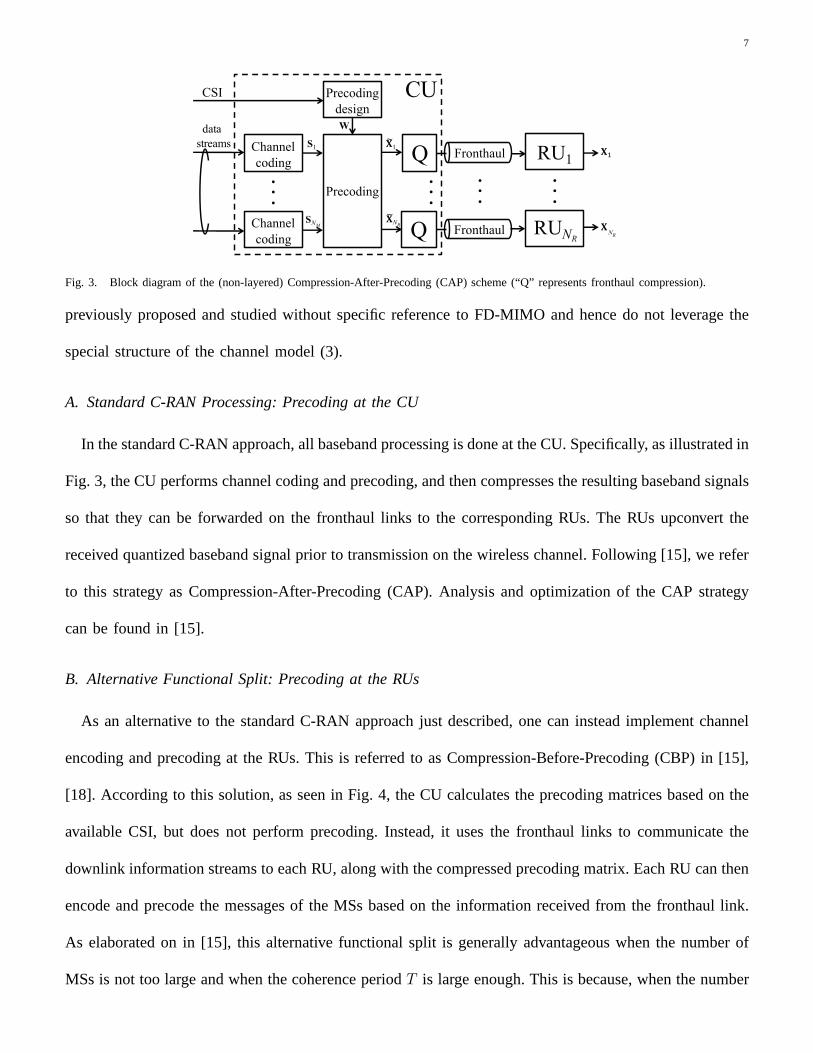
links can be assumed to be negligible. For the azimuth components, we may adopt either a CAP or CBP

approach, as discussed next.
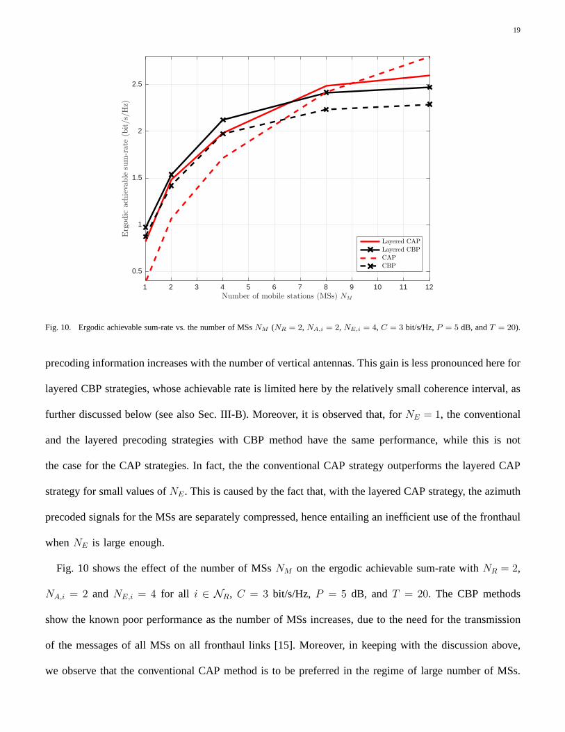
10

Q-1 Kronecker

product

RU1

Channel

coding

Channel

coding

.

.

.

Azimuth

precoding

Azimuth

precoding

design

Current

CSI

Q...

CU

.

.

.

S1

SNM

!"#$

data

streamsFronthaul

FronthaulQ

%$

%#&

Q-1 Kronecker

product

%NR

&RUNR

Elevation

precoding

design

Long-term

CSI Negligible fronthaul overhead

!#

!NR

!"NR

$

!"#$

!"NR

$

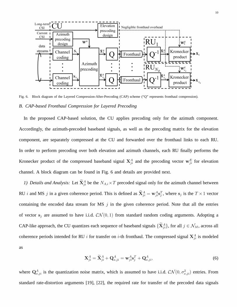
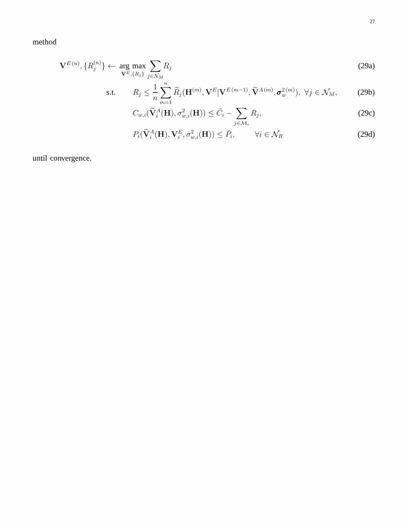
Fig. 6. Block diagram of the Layered Compression-After-Precoding (CAP) scheme (“Q” represents fronthaul compression).

B. CAP-based Fronthaul Compression for Layered Precoding

In the proposed CAP-based solution, the CU applies precoding only for the azimuth component.

Accordingly, the azimuth-precoded baseband signals, as well as the precoding matrix for the elevation

component, are separately compressed at the CU and forwarded over the fronthaul links to each RU.

In order to perform precoding over both elevation and azimuth channels, each RU finally performs the

Kronecker product of the compressed baseband signalXAji and the precoding vectorwE

ji for elevation

channel. A block diagram can be found in Fig. 6 and details areprovided next.

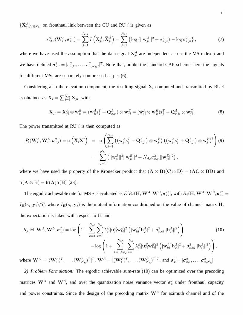
1) Details and Analysis: Let XAji be theNA,i×T precoded signal only for the azimuth channel between

RU i and MSj in a given coherence period. This is defined asXAji = wA

jisTj , wheresj is theT ×1 vector

containing the encoded data stream for MSj in the given coherence period. Note that all the entries

of vector sj are assumed to have i.i.d.CN (0, 1) from standard random coding arguments. Adopting a

CAP-like approach, the CU quantizes each sequence of baseband signals{XAji}, for all j ∈ NM , across all

coherence periods intended for RUi for transfer oni-th fronthaul. The compressed signalXAji is modeled

as

XAji = XA

ji +QAx,ji = wA

jisTj +QA

x,ji, (6)

whereQAx,ji is the quantization noise matrix, which is assumed to have i.i.d. CN (0, σ2

x,ji) entries. From

standard rate-distortion arguments [19], [22], the required rate for transfer of the precoded data signals

11

{XAji}j∈NM

on fronthaul link between the CU and RUi is given as

Cx,i(WAi ,σσσ

2x,i) =

NM∑

j=1

I(XA

ji; XAji

)=

NM∑

j=1

{log(||wA

ji||2 + σ2x,ji

)− log σ2

x,ji

}, (7)

where we have used the assumption that the data signalXAji are independent across the MS indexj and

we have definedσσσ2x,i = [σ2

x,1i, . . . , σ2x,NM i]

T . Note that, unlike the standard CAP scheme, here the signals

for different MSs are separately compressed as per (6).

Considering also the elevation component, the resulting signal Xi computed and transmitted by RUi

is obtained asXi =∑NM

j=1Xji, with

Xji = XAji ⊗wE

ji = (wAjis

Tj +QA

x,ji)⊗wEji = (wA

ji ⊗wEji)s

Tj +QA

x,ji ⊗wEji. (8)

The power transmitted at RUi is then computed as

Pi(WAi ,W

Ei ,σσσ

2x,i) = tr

(XiX

†i

)= tr

(NM∑

j=1

((wA

jisTj +QA

x,ji

)⊗wE

ji

) ((wA

jisTj +QA

x,ji

)⊗wE

ji

)†)

(9)

=

NM∑

j=1

(||wA

ji||2||wEji||2 +NA,iσ

2x,ji||wE

ji||2),

where we have used the property of the Kronecker product that(A ⊗ B)(C ⊗D) = (AC ⊗ BD) and

tr(A⊗B) = tr(A)tr(B) [23].

The ergodic achievable rate for MSj is evaluated asE[Rj(H,WA,WE,σσσ2x)], with Rj(H,WA,WE,σσσ2

x) =

IH(sj;yj)/T , whereIH(sj ;yj) is the mutual information conditioned on the value of channel matrix H,

the expectation is taken with respect toH and

Rj(H,WA,WE,σσσ2x) = log

(1 +

NM∑

k=1

NR∑

i=1

λEji|uE

jiwEki|2(|wA †

ki hAji|2 + σ2

x,ki||hAji||2))

(10)

− log

(1 +

NM∑

k=1,k 6=j

NR∑

i=1

λEji|uE

jiwEki|2(|wA †

ki hAji|2 + σ2

x,ki||hAji||2))

,

whereWA = [(WA1 )

T , . . . , (WANR

)T ]T , WE = [(WE1 )

T , . . . , (WENR

)T ]T , andσσσ2x = [σσσ2

x,1, . . . ,σσσ2x,NR

].

2) Problem Formulation: The ergodic achievable sum-rate (10) can be optimized over the precoding

matricesWA and WE, and over the quantization noise variance vectorσσσ2x under fronthaul capacity

and power constraints. Since the design of the precoding matrix WA for azimuth channel and of the

12

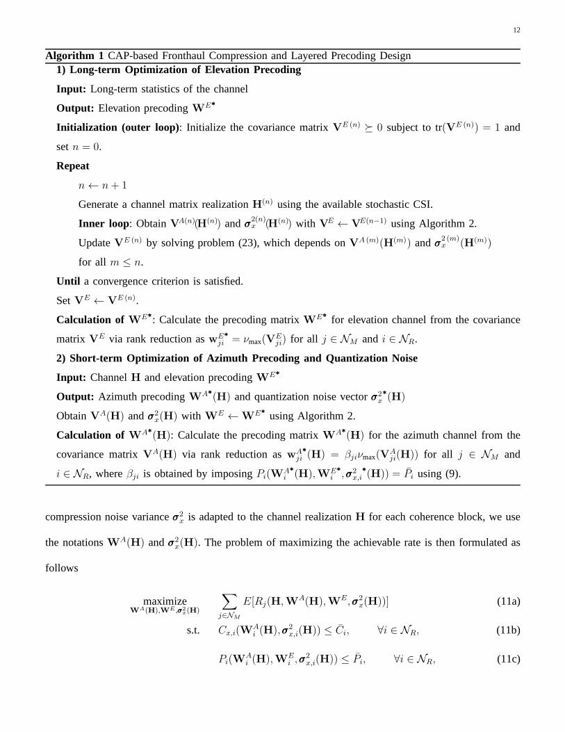
Algorithm 1 CAP-based Fronthaul Compression and Layered Precoding Design1) Long-term Optimization of Elevation Precoding

Input: Long-term statistics of the channel

Output: Elevation precodingWE∗∗∗

Initialization (outer loop): Initialize the covariance matrixVE (n) � 0 subject to tr(VE (n)) = 1 and

setn = 0.

Repeat

n← n+ 1

Generate a channel matrix realizationH(n) using the available stochastic CSI.

Inner loop: ObtainVA(n)(H(n)) andσσσ2(n)x (H(n)) with VE ← VE(n−1) using Algorithm 2.

UpdateVE (n) by solving problem (23), which depends onVA (m)(H(m)) andσσσ2 (m)x (H(m))

for all m ≤ n.

Until a convergence criterion is satisfied.

SetVE ← VE (n).

Calculation of WE∗∗∗: Calculate the precoding matrixWE∗∗∗ for elevation channel from the covariance

matrix VE via rank reduction aswEji

∗∗∗= νmax(V

Eji) for all j ∈ NM and i ∈ NR.

2) Short-term Optimization of Azimuth Precoding and Quantization Noise

Input: ChannelH and elevation precodingWE∗∗∗

Output: Azimuth precodingWA∗∗∗(H) and quantization noise vectorσσσ2

x∗∗∗(H)

ObtainVA(H) andσσσ2x(H) with WE ←WE∗∗∗

using Algorithm 2.

Calculation of WA∗∗∗(H): Calculate the precoding matrixWA∗∗∗

(H) for the azimuth channel from the

covariance matrixVA(H) via rank reduction aswAji

∗∗∗(H) = βjiνmax(V

Aji(H)) for all j ∈ NM and

i ∈ NR, whereβji is obtained by imposingPi(WAi

∗∗∗(H),WE

i

∗∗∗,σσσ2

x,i∗∗∗(H)) = Pi using (9).

compression noise varianceσσσ2x is adapted to the channel realizationH for each coherence block, we use

the notationsWA(H) andσσσ2x(H). The problem of maximizing the achievable rate is then formulated as

follows

maximizeWA(H),WE ,σσσ2

x(H)

j∈NM

E[Rj(H,WA(H),WE,σσσ2x(H))] (11a)

s.t. Cx,i(WAi (H),σσσ2

x,i(H)) ≤ Ci, ∀i ∈ NR, (11b)

Pi(WAi (H),WE

i ,σσσ2x,i(H)) ≤ Pi, ∀i ∈ NR, (11c)

13

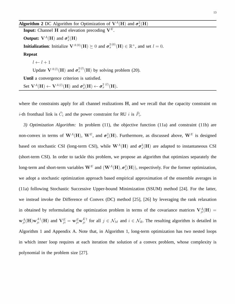
Algorithm 2 DC Algorithm for Optimization ofVA(H) andσσσ2x(H)

Input: ChannelH and elevation precodingVE.

Output: VA(H) andσσσ2x(H)

Initialization: Initialize VA (0)(H) � 0 andσσσ2 (0)x (H) ∈ R

+, and setl = 0.

Repeat

l ← l + 1

UpdateVA (l)(H) andσσσ2 (l)x (H) by solving problem (20).

Until a convergence criterion is satisfied.

SetVA(H)← VA (l)(H) andσσσ2x(H)← σσσ

2 (l)x (H).

where the constraints apply for all channel realizationsH, and we recall that the capacity constraint on

i-th fronthaul link isCi and the power constraint for RUi is Pi.

3) Optimization Algorithm: In problem (11), the objective function (11a) and constraint (11b) are

non-convex in terms ofWA(H), WE, andσσσ2x(H). Furthermore, as discussed above,WE is designed

based on stochastic CSI (long-term CSI), whileWA(H) andσσσ2x(H) are adapted to instantaneous CSI

(short-term CSI). In order to tackle this problem, we propose an algorithm that optimizes separately the

long-term and short-term variablesWE and(WA(H),σσσ2x(H)), respectively. For the former optimization,

we adopt a stochastic optimization approach based empirical approximation of the ensemble averages in

(11a) following Stochastic Successive Upper-bound Minimization (SSUM) method [24]. For the latter,

we instead invoke the Difference of Convex (DC) method [25],[26] by leveraging the rank relaxation

in obtained by reformulating the optimization problem in terms of the covariance matricesVAji(H) =

wAji(H)wA †

ji (H) andVEji = wE

jiwE †ji for all j ∈ NM and i ∈ NR. The resulting algorithm is detailed in

Algorithm 1 and Appendix A. Note that, in Algorithm 1, long-term optimization has two nested loops

in which inner loop requires at each iteration the solution of a convex problem, whose complexity is

polynomial in the problem size [27].

14

MUX...

CU

MUX

Q

Q

.

.

.

De-

MUX

De-

MUX

Q-1

Pre-

coding

Pre-

coding

RU1

RUNRdata

streams

Cluster-

ing

Fronthaul

Fronthaul

Channel

coding

!"#

!"$

!NR

$

Current

CSI

Elevation

precoding

design

Long-term

CSI

Azimuth

precoding

design

Kronecker

product

Channel

coding

Q-1

Kronecker

product

!NR

#

Negligible fronthaul overhead

!% "$

!%NR

$

!% "$

!%NR

$

&"

&NR

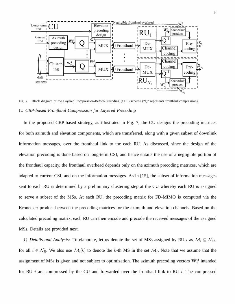
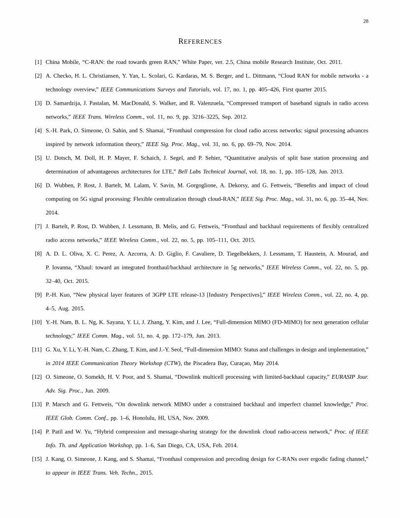
Fig. 7. Block diagram of the Layered Compression-Before-Precoding (CBP) scheme (“Q” represents fronthaul compression).

C. CBP-based Fronthaul Compression for Layered Precoding

In the proposed CBP-based strategy, as illustrated in Fig. 7, the CU designs the precoding matrices

for both azimuth and elevation components, which are transferred, along with a given subset of downlink

information messages, over the fronthaul link to the each RU. As discussed, since the design of the

elevation precoding is done based on long-term CSI, and hence entails the use of a negligible portion of

the fronthaul capacity, the fronthaul overhead depends only on the azimuth precoding matrices, which are

adapted to current CSI, and on the information messages. As in [15], the subset of information messages

sent to each RU is determined by a preliminary clustering step at the CU whereby each RU is assigned

to serve a subset of the MSs. At each RU, the precoding matrix for FD-MIMO is computed via the

Kronecker product between the precoding matrices for the azimuth and elevation channels. Based on the

calculated precoding matrix, each RU can then encode and precode the received messages of the assigned

MSs. Details are provided next.

1) Details and Analysis: To elaborate, let us denote the set of MSs assigned by RUi asMi ⊆ NM ,

for all i ∈ NR. We also useMi[k] to denote thek-th MS in the setMi. Note that we assume that the

assignment of MSs is given and not subject to optimization. The azimuth precoding vectorsWAi intended

for RU i are compressed by the CU and forwarded over the fronthaul link to RU i. The compressed

15

azimuth precodingWAi for RU i at the CU is then given by

WAi = WA

i +Qw,i, (12)

where the quantization noise matrixQw,i is assumed to have zero-mean i.i.d.CN (0, σ2w,i) entries. The

required rate for the transfer of the azimuth precoding on fronthaul link is given, similar to (7), as

Cw,i(WAi , σ

2w,i) =

1

TI(WA

i ;WAi

)(13)

=1

T{log det

(WA

i WA †i + σ2

w,iI)− log det

(σ2w,iI)},

whereWAi = [wA

Mi[1] i, . . . , wA

Mi[|Mi|] i]. The remaining fronthaul capacity is used to convey information

messages, whose total rate is∑

j∈MiRj with Rj being the user rate for MSj. At each RUi, the precoding

matrix for FD-MIMO is obtained via the Kronecker product of the elevation and azimuth components,

yielding the transmitted signalXi =∑

j∈MiXji, with

Xji = (wAji ⊗wE

ji)sTj = (wA

ji ⊗wEji)s

Tj + qA

w,jisTj ⊗wE

ji. (14)

The power transmitted at RUi is then calculated as

Pi(WAi ,W

Ei , σ

2w,i) = tr

(XiX

†i

)=∑

j∈Mi

(||wA

ji||2||wEji||2 +NA,iσ

2w,i||wE

ji||2). (15)

The ergodic achievable rate for MSj is calculated asE[Rj(H,WA,WE,σσσ2w)] with

Rj(H,WA,WE,σσσ2w) = log

(1 +

NR∑

i=1

k∈Mi

λEji|uE

jiwEki|2(|wA †

ki hAji|2 + σ2

w,i||hAji||2))

(16)

− log

1 +

NR∑

i=1

k∈Mi\j

λEji|uE

jiwEki|2(|wA †

ki hAji|2 + σ2

w,i||hAji||2) ,

whereWA = [WAT1 , . . . ,WAT

NR]T andσσσ2

w = [σ2w,1, . . . , σ

2w,NR

].

2) Problem Formulation: As discussed in Section IV-B, the azimuth precodingWA(H) and the

compression noise varianceσσσ2w(H) can be adapted to the current channel realization at each coherence

block. Accordingly, the optimization problem of interest can be formulated as

16

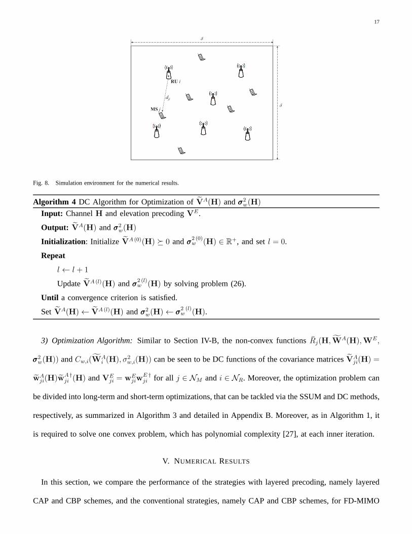
Algorithm 3 CBP-based Fronthaul Compression and Layered Precoding Design1) Long-term Optimization of Elevation Precoding and User Rates

Input: Long-term statistics of the channel and clustering{Mi}Output: Elevation precodingWE ∗ and MSs’ rates{Rj}Initialization (outer loop): Initialize the covariance matrixVE (n) � 0 subject to tr(VE (n)) = 1 and

{R(n)j } ∈ R

+, and setn = 0.

Repeat

n← n+ 1

Generate a channel matrix realizationH(n) using the available stochastic CSI.

Inner loop: ObtainVA(n)(H(n)) andσσσ2(n)w (H(n)) with VE ← VE(n−1) using Algorithm 4.

UpdateVE (n) and{R(n)j } by solving problem (29), which depends onVA (m)(H(m)) and

σσσ2 (m)w (H(m)) for all m ≤ n.

Until a convergence criterion is satisfied.

SetVE ← VE (n) and{Rj} ← {R(n)j }.

Calculation of WE∗∗∗: Calculate the precoding matrixWE∗∗∗ for elevation channel from the covariance

matrix VE via rank reduction aswEji

∗∗∗= νmax(V

Eji) for all j ∈ NM and i ∈ NR.

2) Short-term Optimization of Azimuth Precoding and Quantization Noise

Input: ChannelH and elevation precodingWE∗∗∗

Output: Azimuth precodingWA∗∗∗(H) and quantization noise vectorσσσ2w∗∗∗(H)

ObtainVA(H) andσσσ2w(H) with WE ←WE∗∗∗

using Algorithm 4.

Calculation of WA∗∗∗(H): Calculate the precoding matrixWA∗∗∗(H) for the azimuth channel from the

covariance matrixVA(H) via rank reduction aswA∗∗∗ji (H) = βjiνmax(V

Aji(H)) for all j ∈ NM and

i ∈ NR, whereβji is obtained by imposingPi(WA∗∗∗i (H),WE

i , σ2w,i

∗∗∗(H)) = Pi using (15).

maximizeWA(H),WE ,{Rj},σσσ2

w(H)

j∈NM

Rj (17a)

s.t. Rj ≤ E[Rj(H,WA(H),WE,σσσ2w(H))], ∀j ∈ NM , (17b)

Cw,i(WAi (H), σ2

w,i(H)) ≤ Ci −∑

j∈Mi

Rj , ∀i ∈ NR, (17c)

Pi(WAi (H),WE

i , σ2w,i(H)) ≤ Pi, ∀i ∈ NR, (17d)

where the constraints apply to every channel realizationH.

17

d

d

dji

RU i

MS j

Fig. 8. Simulation environment for the numerical results.

Algorithm 4 DC Algorithm for Optimization ofVA(H) andσσσ2w(H)

Input: ChannelH and elevation precodingVE.

Output: VA(H) andσσσ2w(H)

Initialization: Initialize VA (0)(H) � 0 andσσσ2 (0)w (H) ∈ R

+, and setl = 0.

Repeat

l ← l + 1

UpdateVA (l)(H) andσσσ2 (l)w (H) by solving problem (26).

Until a convergence criterion is satisfied.

Set VA(H)← VA (l)(H) andσσσ2w(H)← σσσ

2 (l)w (H).

3) Optimization Algorithm: Similar to Section IV-B, the non-convex functionsRj(H,WA(H),WE,

σσσ2w(H)) andCw,i(W

Ai (H), σ2

w,i(H)) can be seen to be DC functions of the covariance matricesVAji(H) =

wAji(H)wA †

ji (H) andVEji = wE

jiwE †ji for all j ∈ NM andi ∈ NR. Moreover, the optimization problem can

be divided into long-term and short-term optimizations, that can be tackled via the SSUM and DC methods,

respectively, as summarized in Algorithm 3 and detailed in Appendix B. Moreover, as in Algorithm 1, it

is required to solve one convex problem, which has polynomial complexity [27], at each inner iteration.

V. NUMERICAL RESULTS

In this section, we compare the performance of the strategies with layered precoding, namely layered

CAP and CBP schemes, and the conventional strategies, namely CAP and CBP schemes, for FD-MIMO

18

1 2 3 4 5 6 7 8Number of vertical antennas NE

0.2

0.3

0.4

0.5

0.6

0.7

0.8

Ergodic

achievable

sum-rate

(bit/s/Hz)

Layered CAPLayered CBPCAPCBP

Fig. 9. Ergodic achievable sum-rate vs. the number of vertical antennasNE (NR = NM = 2, NA,i = 2, C = 1 bit/s/Hz,P = 0 dB, and

T = 20).

systems. To this end, we consider a set-up simulation environment where the RUs and MSs are randomly

located in a square area with sideδ = 500 m as in Fig. 8. In the path loss formula (4), we set the

reference distance tod0 = 50 m and the path loss exponent toη = 3 with dji being the Euclidean distance

between thei-th RU and thej-th MS. The channels are assumed to have the Kronecker model in (3).

Throughout, we assume that the every RU is subject to the samefronthaul capacityC and has the same

power constraintP , namelyCi = C and Pi = P for i ∈ NR. Throughout, we consider CBP strategies in

which each RU serves all MSs, i.e.,NC = NM .

Fig. 9 shows the ergodic achievable sum-rate as function of the number of vertical antennasNE, where

the number of RUs and MSs isNR = NM = 2, the number of horizontal antennas isNA,i = 2 for all

i ∈ NR, the fronthaul capacity isC = 1 bit/s/Hz, the transmit power isP = 0 dB and the coherence time

is T = 20. We observe that the layered precoding schemes provide increasingly large gains asNE grows

larger. This is because, in the conventional strategies, the fronthaul overhead for the transfer of elevation

19

1 2 3 4 5 6 7 8 9 10 11 12Number of mobile stations (MSs) NM

0.5

1

1.5

2

2.5

Ergodic

achievable

sum-rate

(bit/s/Hz)

Layered CAPLayered CBPCAPCBP

Fig. 10. Ergodic achievable sum-rate vs. the number of MSsNM (NR = 2, NA,i = 2, NE,i = 4, C = 3 bit/s/Hz,P = 5 dB, andT = 20).

precoding information increases with the number of vertical antennas. This gain is less pronounced here for

layered CBP strategies, whose achievable rate is limited here by the relatively small coherence interval, as

further discussed below (see also Sec. III-B). Moreover, itis observed that, forNE = 1, the conventional

and the layered precoding strategies with CBP method have the same performance, while this is not

the case for the CAP strategies. In fact, the the conventional CAP strategy outperforms the layered CAP

strategy for small values ofNE . This is caused by the fact that, with the layered CAP strategy, the azimuth

precoded signals for the MSs are separately compressed, hence entailing an inefficient use of the fronthaul

whenNE is large enough.

Fig. 10 shows the effect of the number of MSsNM on the ergodic achievable sum-rate withNR = 2,

NA,i = 2 and NE,i = 4 for all i ∈ NR, C = 3 bit/s/Hz, P = 5 dB, andT = 20. The CBP methods

show the known poor performance as the number of MSs increases, due to the need for the transmission

of the messages of all MSs on all fronthaul links [15]. Moreover, in keeping with the discussion above,

we observe that the conventional CAP method is to be preferred in the regime of large number of MSs.

20

1 2 3 4 5 6 7 8 9 10Fronthaul capacity C (bit/s/Hz)

0.4

0.6

0.8

1

1.2

1.4

1.6

1.8

Ergodic

achievable

sum-rate

(bit/s/Hz)

Layered CAPLayered CBPCAPCBP

Fig. 11. Ergodic achievable sum-rate vs. the fronthaul capacity C (NR = 2, NM = 2, NA,i = 2, NE,i = 4, P = 5 dB, andT = 10).

This is due to the separate compression of the azimuth precoded signals of layered CAP, which entails a

fronthaul overhead proportional to the number of MSs.

In Fig. 11, the ergodic achievable sum-rate is plotted versus the fronthaul capacityC for NR = NM = 2,

NA,i = 2 andNE,i = 4 for all i ∈ NR, P = 5 dB, andT = 10. We first remark that the performance gain

of the layered strategies is observed at low-to-moderate fronthaul capacities, while, for large fronthaul

capacities, the performance of the conventional strategies approach that of the layered strategies. As a

general rule, the conventional CAP strategy is uniformly better than conventional CBP as long as the

fronthaul capacity is sufficiently large, due to the enhanced interference mitigation capabilities of CAP

[15]. Instead, the layered CAP strategy is advantageous here across all values of fronthaul capacity.

The effect of the coherence timeT is investigated in Fig. 12, withNR = NM = 2, NA,i = 2 and

NE,i = 4 for all i ∈ NR, C = 4 bit/s/Hz, andP = 5 dB. The CBP schemes benefit from a larger

coherence timeT , since the fronthaul overhead required to transmit precoding information gets amortized

over a larger period. In contrast, such overhead in layered CAP and CAP schemes scales proportionally

21

2 4 6 8 10 12 14 16 18 20Coherence time T

0.4

0.6

0.8

1

1.2

1.4

1.6

Ergodic

achievable

sum-rate

(bit/s/Hz)

Layered CAPLayered CBPCAPCBP

Fig. 12. Ergodic achievable sum-rate vs. the coherence timeT (NR = NM = 2, NA,i = 2, NE,i = 4, C = 4 bit/s/Hz, andP = 5 dB).

to the coherence timeT and hence the layered CAP and CAP schemes are not affected by the coherence

time.

VI. CONCLUDING REMARKS

In this paper, we have studied the design of downlink Cloud Radio Access Network (C-RAN) systems

in which the Radio Units (RUs) are equipped with Full Dimensional (FD)-MIMO arrays. We proposed to

leverage the special low-rank structure of FD-MIMO channel, which exhibits different rates of variability

in the elevation and azimuth components, by means of a novel layered precoding strategy coupled with

an adaptive fronthaul compression scheme. Specifically, inthe layered strategy, a single precoding matrix

is optimized for the elevation channel across all coherencetimes based on long-term Channel State

Information (CSI), while azimuth precoding matrices are optimized across independent coherence interval

by adapting to instantaneous CSI. This proposed layered approach has the unique advantage in a C-RAN

of potentially reducing the fronthaul overhead, due to the opportunity to amortize the overhead related to

the elevation channel component across multiple coherencetimes. Via numerical results, it is shown that

22

the layered strategies significantly outperform standard non-layered schemes, especially in the regime of

low fronthaul capacity and large number of vertical antennas.

We have also considered two different functional splits forboth layered and non-layered precod-

ing, namely the conventional C-RAN implementation, also known as Compress-After-Precoding (CAP)

scheme, and an alternative split, referred to as Compress-Before-Precoding (CBP), whereby channel

coding and precoding are performed at the RUs. Layered precoding is seen to work better under a

CAP implementation when the coherence interval is not too large and the number of vertical antennas is

sufficiently large; whereas the CBP approach benefits from a longer coherence interval due to its capability

to amortize the fronthaul overhead for transfer of azimuth precoding information. Interesting open issues

include the investigation of a scenario with multiple interfering clusters of RUs controlled by distinct

Central Units (CUs) (see [28]), and the analysis of the performance in the presence of more general

FD-MIMO channel models (see, e.g., [11]).

APPENDIX A

OPTIMIZATION ALGORITHM FOR THE LAYERED CAP STRATEGY

In this Appendix, we detail the derivation of Algorithm 1 forthe optimization of the layered CAP

strategy. We first discuss the optimization problem for the short-term variables, namely the covariance

matrixVA(H) for azimuth precoding and the quantization noise varianceσσσ2x(H), which are adapted to the

channel realizationH, for given the elevation covariance matrixVE. We then consider the optimization

of the long-term variable, namely the covariance matrixVE for elevation precoding, with the given

covariance matricesVA(H) for azimuth precoding and quantization noise vectorsσσσ2x(H).

After obtaining the elevation covariance matrixVE∗∗∗, using the approach in Algorithm 1, the precoding

matrixWE∗∗∗ for the elevation channel is calculated via the principal eigenvector approximation [29] of the

obtained solutionVE∗∗∗aswE

ji

∗∗∗= νmax(V

Eji

∗∗∗) for all j ∈ NM andi ∈ NR. In a similar fashion, the algorithm

obtains the precoding matrixWA∗∗∗(H) for the azimuth channel via the standard rank-reduction approach

[29] from the obtained solutionVA(H)∗∗∗ aswA

ji

∗∗∗(H) = βjiνmax(V

Aji(H)

∗∗∗) with the normalization factors

23

βji selected to satisfy the power constraint with equality, namely Pi(WAi

∗∗∗(H),WE

i

∗∗∗,σσσ2

x,i∗∗∗(H)) = Pi.

A. Optimization over VA(H) and σσσ2x(H) with given VE

Here, we tackle the problem (11) based on the DC algorithm [25] given the elevation precoding

covariance matrixVE over the azimuth covariance matrixVA(H) and the quantization noise variance

σσσ2x(H). To this end, the objective functionRj(H,WA(H),WE,σσσ2

x(H)) is approximated by a locally

tight lower boundRj(H,VA(H), σσσ2x(H)|VA (l−1)(H),σσσ

2 (l−1)x (H),VE) around solutionsVA (l−1)(H) and

σσσ2 (l−1)x (H) obtained at(l − 1)-th inner iteration with

Rj(H,VA(H),σσσ2x(H)|VA (l−1)(H),σσσ2 (l−1)

x (H),VE) = log

(1 +

NM∑

k=1

NR∑

i=1

ρji(VAki(H),VE

ki, σ2x,ki(H))

)(18)

−f(1+

NM∑

k=1,k 6=j

NR∑

i=1

ρji(VA (l−1)ki (H),VE

ki,σσσ2 (l−1)x,ki (H)), 1+

NM∑

k=1,k 6=j

NR∑

i=1

ρji(VAki(H),VE

ki, σ2x,ki(H))

)

whereρji(VAki,V

Eki, σ

2x,ki) = λE

jiuEjiV

Ekiu

†ji

(hAjiV

Akih

A †ji + σ2

x,ki||hAji||2)

and the linearized functionf(a, b)

is obtained from the first-order Taylor expansion of the log function asf(a, b) = log(a)+(b− a)/a. Since

the fronthaul constraint (11b) is a DC constraint, the left-hand side of the constraint (11b) is approximated

by applying successive locally tight convex lower bounds as

Cx,i(VAi (H),σσσ2

x,i(H)|VA (l−1)i (H),σσσ

2 (l−1)x,i (H)) , (19)

NM∑

j=1

{f(

tr(VA (l−1)ji (H)) + σ

2 (l−1)x,ji (H), tr(VA

ji(H)) + σ2x,ji(H)

)− log σ2

x,ji

}.

At l-th inner loop, the following convex optimization problem,for given VA (l−1)(H), σσσ2 (l−1)x (H), and

VE, is solved for obtaining new iteratesVA (l)(H) andσσσ2 (l)x (H) as

VA (l)(H),σσσ2 (l)x (H)← arg max

VA(H),σσσ2x(H)

j∈NM

Rj(H,VA(H),σσσ2x(H)|VA (l−1)(H),σσσ2 (l−1)

x (H),VE) (20a)

s.t. Cx,i(VAi (H),σσσ2

x,i(H)|VA (l−1)i (H),σσσ

2 (l−1)x,i (H)) ≤ Ci, (20b)

Pi(VAi (H),VE

i ,σσσ2x,i(H)) ≤ Pi, ∀i ∈ NR. (20c)

The DC method obtains the solutionsVA(H) andσσσ2x(H) by solving the problem (20) iteratively overl

until a convergence criterion is satisfied and the resultingalgorithm is summarized in Algorithm 2.

24

B. Optimization over VE

In this part, the covariance matrixVE for elevation precoding is designed for given azimuth precoding

covariance matricesVA (m) = VA (m)(H(m)) and quantization noise vectorsσσσ2 (m)x = σσσ

2 (m)x (H(m)) for all

m = 1, . . . , n. Since the elevation covariance matrixVE (n) is not adapted to the channel realizationH and

the objective function (11) is non-convex with respect toVE (n), in this optimization, we use the SSUM

algorithm [24]. To this end, at each step, a stochastic lowerbound of the objective function is maximized

around the current iterate. Following the SSUM method, atn-th outer loop, the objective function with

givenVA (m) andσσσ2 (m)x , for all m = 1, . . . , n, is reformulated as the empirical average

1

n

n∑

m=1

Rj(H(m),VE|VE (m−1),VA (m),σσσ2 (m)

x ), (21)

whereRj(H(m),VE|VE (m−1),VA,σσσ2

x) is a locally tight convex lower bound around the previous iterate

VE (m−1), when the channel realization isH(m), and is calculated as

Rj(H(m),VE|VE (m−1),VA (m),σσσ2 (m)

x ) = log

(1 +

NM∑

k=1

NR∑

i=1

ρji(H(m),V

A (m)ki ,VE

ki, σ2 (m)x,i )

)(22)

−f(1 +

NM∑

k=1,k 6=j

NR∑

i=1

ρki(H(m),V

A (m)ki ,V

E (m−1)ki ,σσσ

2 (m)x,i ), 1 +

NM∑

k=1,k 6=j

NR∑

i=1

ρki(H(m),V

A (m)ki ,VE

ki, σ2 (m)x,i )

),

with ρji(H(m),VA

ki,VEki, σ

2x,i) = λ

E (m)ji u

E (m)ji VE

kiu(m) †ji (h

A (m)ji VA

kihA (m) †ji +σ2

x,i||hA (m)ji ||2). Then-th iterate

VE (n) is obtained by solving the following convex optimization problem

VE (n) ← arg maxVE

1

n

n∑

m=1

j∈NM

Rj(H(m),VE|VE (m−1),VA (m),σσσ2 (m)

x ) (23a)

s.t. Cx,i(VA (n)i ,σσσ

2 (n)x,i ) ≤ Ci, ∀i ∈ NR, (23b)

Pi(VA (n)i ,VE

i ,σσσ2 (n)x,i ) ≤ Pi, ∀i ∈ NR. (23c)

As in Section A-A, the outer loop in Algorithm 1 is repeated until the convergence is achieved.

APPENDIX B

OPTIMIZATION ALGORITHM FOR LAYERED CBP STRATEGY

In this Appendix, the precoding matricesWE∗∗∗ andWA∗∗∗, MSs’ rates{Rj} and quantization noise vector

σσσ2w

∗∗∗ are jointly optimized for the CBP-based strategy. The optimization of short-term variables, namely the

25

covariance matrixVA(H) for azimuth precoding and the quantization noise varianceσσσ2w(H), which are

adapted to the channel realizationH for given the elevation covariance matrixVE, is described first. Then,

the optimization over the long-term variables, namely the covariance matrixVE for elevation precoding

and the user rates{Rj}, is discussed given covariance matricesVA (m)(H) for azimuth precoding and

quantization noise vectorsσσσ2 (m)w (H), for all m = 1, . . . , n, as detailed in Appendix B-B.

As in Appendix A, the elevation precoding matrixWE∗∗∗ and the azimuth precoding matrixWA∗∗∗

are calculated via the standard rank-reduction approach [29] with the obtained solutionsVE∗∗∗ and VA∗∗∗,

respectively, as detailed in Algorithm 3.

A. Optimization over VA(H) and σσσ2w(H) with given VE

Here, we aim at maximizing the objective function (17a) overthe azimuth precoding covariance matrix

VA(H) and the quantization noise varianceσσσ2w(H) given the elevation precoding covariance matrix

VE using the DC method [25]. At thel-th iteration of the DC method, the non-convex functions

Rj(H, VA(H),VE,σσσ2w(H)) and Cw,i(V

Ai (H), σ2

w,i(H)) are respectively substituted with a locally tight

lower boundRj(H, VA(H),σσσ2w(H)| VA (l−1)(H),σσσ

2 (l−1)w (H),VE) and a tight upper boundCw,i(V

Ai (H),

σ2w,i(H)|VA (l−1)

i (H), σ2 (l−1)w,i (H)), obtained as in Appendix A. The bounds are given by

Rj(H, VA(H),σσσ2w(H)|VA (l−1)(H),σσσ2 (l−1)

w (H),VE) = log

(1 +

NR∑

i=1

k∈Mi

ρji(VAki(H),VE

ki, σ2w,i(H))

)

−f

1+

NR∑

i=1

k∈Mi\j

ρki(VA (l−1)ki (H),VE

ki, σ2 (l−1)w,i (H)), 1+

NR∑

i=1

k∈Mi\j

ρki(VAki(H),VE

ki, σ2w,i(H))

, (24)

and

Cw,i(VAi (H), σ2

w,i(H)|VA (l−1)i (H), σ

2 (l−1)w,i (H)) , (25)

1

T

{f(V

A (l−1)i (H) + σ

2 (l−1)w,i (H)I, VA

i (H) + σ2w,i(H)I

)−NA,i log

(σ2w,i

)},

whereρji(VAki,V

Eki, σ

2w,i) = λE

jiuEjiV

Ekiu

†ji

(hAjiV

Akih

A †ji + σ2

w,i||hAji||2)

and the linearization functionf(A,B)

for the matrices is defined asf(A,B) , log det(A) + tr(A−1(B−A)).

26

At l-th iteration of DC method, the following convex optimization problem for givenVA (l−1)(H),

σσσ2 (l−1)w (H) andVE is solved for obtaining new iteratesVA (l)(H) andσσσ2 (l)

w (H):

VA (l)(H),σσσ2 (l)w (H)← arg max

VA(H),σσσ2w(H),{Rj}

j∈NM

Rj (26a)

s.t. Rj ≤ Rj(H, VA(H),σσσ2w(H)|VA (l−1)(H),σσσ2 (l−1)

w (H),VE), ∀j ∈ NM ,(26b)

Cw,i(VAi (H), σ2

w,i(H)|VA (l−1)i (H), σ

2 (l−1)w,i (H)) ≤ Ci −

j∈Mi

Rj , (26c)

Pi(VAi (H),VE

i , σ2w,i(H)) ≤ Pi, ∀i ∈ NR. (26d)

Problem (26) is solved iteratively overl until convergence and the resulting algorithm is summarized in

Algorithm 4.

B. Optimization over VE and {Rj}

We design the covariance matrixVE for elevation precoding and the user rates{Rj} for given

azimuth precoding covariance matricesVA (m) = VA (m)(H(m)) and quantization noise vectorsσσσ2 (m)w =

σσσ2 (m)w (H(m)) for all m = 1, . . . , n. As in Appendix A, this optimization problem can be tackled via the

SSUM method. To this end, the functionE[Rj(H,WA(H),WE,σσσ2w(H))] in (17b) is approximated with

the stochastic upper bound as

1

n

n∑

m=1

Rj(H(m),VE|VE (m−1), VA (m),σσσ2 (m)

w ), (27)

with

Rj(H(m),VE|VE (m−1), VA (m),σσσ2 (m)

w ) = log

(1 +

NR∑

i=1

k∈Mi

ρji(H(m), V

A (m)ki ,VE

ki, σ2 (m)w,i )

)(28)

−f

1 +

NR∑

i=1

k∈Mi\j

ρki(H(m), V

A (m)ki ,V

E (m−1)ki , σ

2 (m)w,i ), 1 +

NR∑

i=1

k∈Mi\j

ρki(H(m), V

A (m)ki ,VE

ki, σ2 (m)w,i )

,

whereρji(H(m), VAki,V

Eki, σ

2w,i) = λ

E (m)ji u

E (m)ji VE

kiu(m) †ji (h

A (m)ji VA

kihA (m) †ji + σ2

w,i||hA (m)ji ||2). At the n-th

iteration,VE (n) and{R(n)j } are obtained by solving the following optimization problembased on SSUM

27

method

VE (n), {R(n)j } ← arg max

VE ,{Rj}

j∈NM

Rj (29a)

s.t. Rj ≤1

n

n∑

m=1

Rj(H(m),VE|VE (m−1), VA (m),σσσ2 (m)

w ), ∀j ∈ NM , (29b)

Cw,i(VAi (H), σ2

w,i(H)) ≤ Ci −∑

j∈Mi

Rj , (29c)

Pi(VAi (H),VE

i , σ2w,i(H)) ≤ Pi, ∀i ∈ NR (29d)

until convergence.

28

REFERENCES

[1] China Mobile, “C-RAN: the road towards green RAN,” WhitePaper, ver. 2.5, China mobile Research Institute, Oct. 2011.

[2] A. Checko, H. L. Christiansen, Y. Yan, L. Scolari, G. Kardaras, M. S. Berger, and L. Dittmann, “Cloud RAN for mobile networks - a

technology overview,”IEEE Communications Surveys and Tutorials, vol. 17, no. 1, pp. 405–426, First quarter 2015.

[3] D. Samardzija, J. Pastalan, M. MacDonald, S. Walker, andR. Valenzuela, “Compressed transport of baseband signals in radio access

networks,” IEEE Trans. Wireless Comm., vol. 11, no. 9, pp. 3216–3225, Sep. 2012.

[4] S.-H. Park, O. Simeone, O. Sahin, and S. Shamai, “Fronthaul compression for cloud radio access networks: signal processing advances

inspired by network information theory,”IEEE Sig. Proc. Mag., vol. 31, no. 6, pp. 69–79, Nov. 2014.

[5] U. Dotsch, M. Doll, H. P. Mayer, F. Schaich, J. Segel, and P. Sehier, “Quantitative analysis of split base station processing and

determination of advantageous architectures for LTE,”Bell Labs Technical Journal, vol. 18, no. 1, pp. 105–128, Jun. 2013.

[6] D. Wubben, P. Rost, J. Bartelt, M. Lalam, V. Savin, M. Gorgoglione, A. Dekorsy, and G. Fettweis, “Benefits and impact ofcloud

computing on 5G signal processing: Flexible centralization through cloud-RAN,”IEEE Sig. Proc. Mag., vol. 31, no. 6, pp. 35–44, Nov.

2014.

[7] J. Bartelt, P. Rost, D. Wubben, J. Lessmann, B. Melis, andG. Fettweis, “Fronthaul and backhaul requirements of flexibly centralized

radio access networks,”IEEE Wireless Comm., vol. 22, no. 5, pp. 105–111, Oct. 2015.

[8] A. D. L. Oliva, X. C. Perez, A. Azcorra, A. D. Giglio, F. Cavaliere, D. Tiegelbekkers, J. Lessmann, T. Haustein, A. Mourad, and

P. Iovanna, “Xhaul: toward an integrated fronthaul/backhaul architecture in 5g networks,”IEEE Wireless Comm., vol. 22, no. 5, pp.

32–40, Oct. 2015.

[9] P.-H. Kuo, “New physical layer features of 3GPP LTE release-13 [Industry Perspectives],”IEEE Wireless Comm., vol. 22, no. 4, pp.

4–5, Aug. 2015.

[10] Y.-H. Nam, B. L. Ng, K. Sayana, Y. Li, J. Zhang, Y. Kim, andJ. Lee, “Full-dimension MIMO (FD-MIMO) for next generationcellular

technology,”IEEE Comm. Mag., vol. 51, no. 4, pp. 172–179, Jun. 2013.

[11] G. Xu, Y. Li, Y.-H. Nam, C. Zhang, T. Kim, and J.-Y. Seol, “Full-dimension MIMO: Status and challenges in design and implementation,”

in 2014 IEEE Communication Theory Workshop (CTW), the Piscadera Bay, Curacao, May 2014.

[12] O. Simeone, O. Somekh, H. V. Poor, and S. Shamai, “Downlink multicell processing with limited-backhaul capacity,”EURASIP Jour.

Adv. Sig. Proc., Jun. 2009.

[13] P. Marsch and G. Fettweis, “On downlink network MIMO under a constrained backhaul and imperfect channel knowledge,” Proc.

IEEE Glob. Comm. Conf., pp. 1–6, Honolulu, HI, USA, Nov. 2009.

[14] P. Patil and W. Yu, “Hybrid compression and message-sharing strategy for the downlink cloud radio-access network,” Proc. of IEEE

Info. Th. and Application Workshop, pp. 1–6, San Diego, CA, USA, Feb. 2014.

[15] J. Kang, O. Simeone, J. Kang, and S. Shamai, “Fronthaul compression and precoding design for C-RANs over ergodic fading channel,”

to appear in IEEE Trans. Veh. Techn., 2015.

29

[16] D. Ying, F. W. Vook, T. A. Thomas, D. J. Love, and A. Ghosh,“Kronecker product correlation model and limited feedbackcodebook

design in a 3D channel model,”Proc. IEEE Int. Conf. on Comm., pp. 5865–5870, Sydney, NSW, Australia, Jun. 2014.

[17] A. Alkhateeb, G. Leus, and R. W. H. Jr., “Multi-layer precoding for full-dimensional massive MIMO systems,”Proc. of Asilomar Conf.

on Sign., Syst. and Computers, pp. 815–819, Pacific Grove, CA, USA, Nov. 2014.

[18] S. Park, C.-B. Chae, and S. Bahk, “Before/after precoded massive MIMO in cloud radio access networks,”Proc. IEEE Int. Conf. on

Comm., pp. 169–173, Budapest, Hungary, Jun. 2013.

[19] A. E. Gamal and Y.-H. Kim,Network Information Theory. Cambridge University Press, 2011.

[20] N. Seifi, J. Zhang, R. W. H. Jr., T. Svensson, and M. Coldrey, “Coordinated 3D beamforming for interference management in cellular

networks,” IEEE Trans. Wireless Comm., vol. 13, no. 10, pp. 5396–5410, Oct. 2014.

[21] Z. Zhong, X. Yin, X. Li, and X. Li, “Extension of ITU IMT-advanced channel models for elevation domains and line-of-sight scenarios,”

Proc. IEEE Veh. Technol. Conf., pp. 1–5, Las Vegas, NV, USA, Sep. 2013.

[22] T. M. Cover and J. A. Thomas,Element of Information Theory. John Wiley & Sons, 2006.

[23] M. Brookes, “The matrix reference manual,”[online] http://www.ee.imperial.ac.uk/hp/staff/dmb/matrix/intro.html, 2011.

[24] M. Razaviyayn, M. Sanjabi, and Z.-Q. Luo, “A stochasticsuccessive minimization method for nonsmooth nonconvex optimization with

applications to transceiver design in wireless communication networks,”arXiv:1307.4457.

[25] A. Beck and M. Teboulle, “Gradient-based algorithms with applications to signal recovery problems,”in Convex Optimization in Signal

Processing and Communications, Y. Eldar and D. Palomar, editors, pp. 42-48, Cambridge University Press 2010.

[26] D. R. Hunter and K. Lange, “A tutorial on MM algorithms,”The American Statistician, vol. 58, no. 1, pp. 30–37, Feb. 2004.

[27] S. Boyd and L. Vandenberghe,Convex Optimization. Cambridge University Press, 2004.

[28] S.-H. Park, O. Simeone, O. Sahin, and S. Shamai, “Inter-cluster design of precoding and fronthaul compression for cloud radio access

networks,” IEEE Wireless Comm. Lett., vol. 3, no. 4, pp. 369–372, Aug. 2014.

[29] L. Vandenberghe and S. Boyd, “Semidefinite relaxation of quadratic optimization problems,”SIAM Rev., vol. 38, no. 1, pp. 49–95,

1996.


Recommended