1Linear Model Predictive Control via MultiparametricProgrammingVassilis Sakizlis, Konstantinos I. Kouramas, and Efstratios N. Pistikopoulos
1.1Introduction
Linear systems with input, output, or state constraints are probably the most impor-tant class of systems in practice and the most studied as well. Although, a varietyof control design methods have been developed for linear systems, it is widely ac-cepted that stability and good performance for these systems, especially in the pres-ence of constraints, is guaranteed with a nonlinear control law. The most popularnonlinear control approach for linear systems with constraints is model predictivecontrol or simply MPC which has become the standard for constrained multivari-able control problems in the process industries [24, 25, 35].
MPC is an online constrained optimization method, based on the so-called re-ceding horizon philosophy [24, 25]. At each sampling instant, the measurementsof the current output and/or state of the system are retrieved and an open-loop op-timal control problem is solved over a finite time horizon to obtain the sequence offuture control values. The first value of the sequence is then obtained and the pro-cedure is repeated in the next sampling instant and over a shifted horizon, leadingto a moving horizon policy. Since the objective function and the constraints of theopen-loop optimal control problem can be set to express true performance objec-tives, the benefits of MPC are tremendous; optimality and constraints’ satisfactionbeing obviously its main advantage.
The application of MPC is, nevertheless, rather restricted, considering its profitpotential, due to its online computational requirements which involve the repeti-tive solution of an optimization problem at regular time intervals. This limitationis in spite of the significant advances in the computational power of modern com-puters and in the area of online optimization over the past few years. Thus, it is fairto state that an efficient implementation of online optimization tools relies on aquick and repetitive online computation of optimal control actions. A way to avoidthese repetitive online computations is by using multiparametric programming tech-niques to solve the optimization problem. With this approach, the control variablesare obtained as an explicit function of the state variables and therefore the online
4 1 Linear Model Predictive Control via Multiparametric Programming
optimization breaks down to simple function evaluations, at regular time intervals,to compute the corresponding control actions for the given state of the plant. Thisis known as the online optimization via off-line parametric optimization concept.
1.1.1Multiparametric Programming
Overall, multiparametric programming is a technique for solving any optimizationproblem, where the objective is to minimize or maximize a performance criterionsubject to a given set of constraints and where some of the parameters vary betweenspecified lower and upper bounds. The main characteristic of multiparametric pro-gramming is its ability to obtain [1, 4, 15, 19, 20, 26, 28]
(i) the objective and optimization variable as functions of thevarying parameters, and
(ii) the regions in the space of the parameters where thesefunctions are valid.
Multiparametric programming has been applied to a number of applications listedhere
(i) hybrid parametric/stochastic programming [2, 22],(ii) process planning under uncertainty [29],
(iii) material design under uncertainty [13],(iv) multiobjective optimization [26, 27, 30],(v) flexibility analysis [5],
(vi) computation of singular multivariate normal probabilities[6], and
(vii) model predictive control [9, 10, 31].
The advantage of using multiparametric programming to address these prob-lems is that for problems pertaining to plant operations, such as for process plan-ning, scheduling, and control, one can obtain a complete map of all the optimalsolutions. Hence, as the operating conditions vary, one does not have to reoptimizefor the new set of conditions, since the optimal solution is already available as afunction of the operating conditions. Mathematically, all the above applications canbe generally posed as a multiparametric mixed-integer nonlinear programming(mp-MINLP) problem
z(θ ) = miny,x
dTy + f(x)
s.t. Ey + g(x) ≤ b + Fθ ,θmin ≤ θ ≤ θmax,x ∈ X ⊆ R
n,y ∈ Y = {0, 1}m,θ ∈ � ⊆ R
s,
(1.1)
where y is a vector of {0, 1} binary variables, x is a vector of continuous variables,f a scalar, continuously differentiable and convex function of x, g a vector of con-
1.1 Introduction 5
tinuous differentiable and convex functions of x, b and d are constant vectors, Eand F are constant matrices, θ is a vector of parameters, θmin and θmax are the lowerand upper bounds of θ , and X and � are compact and convex polyhedral sets ofdimensions n and s, respectively.
The detailed theory and algorithms of solving the mp-MINLP problem (1.1) areexploited in [1, 14, 15]. Furthermore, a number of variations of the problem (1.1)have been developed and examined in [2, 14]. A special formulation of (1.1) which,as we will later see in this chapter, is of great importance for linear model predictivecontrol problems is the multiparametric quadratic programming problem in whichd = 0, E = 0, and f and g are quadratic and linear functions of x, respectively. Thiscase will be given our full attention and will be treated carefully in the followingsections of this chapter.
1.1.2Model Predictive Control
Consider the general mathematical description of discrete-time, linear time-invariant systems{
xt+1 = Axt + But
yt = Cxt(1.2)
subject to the following constraints:
ymin ≤ yt ≤ ymax,umin ≤ ut ≤ umax,
(1.3)
where xt ∈ Rn, ut ∈ R
m, and yt ∈ Rp are the state, input, and output vectors,
respectively, subscripts min and max denote lower and upper bounds, respectively,and the matrix pair (A, B) is stabilizable.
The linear MPC problem for regulating (1.2) to the origin is posed as the follow-ing quadratic programming problem [24, 25, 35]
minU
J(U, xt) = x′t+Ny|tPxt+Ny|t +
Ny–1∑k=0
x′t+k|tQxt+k|t + u′
t+kRut+k
s.t. ymin ≤ yt+k|t ≤ ymax, k = 1, . . . , Nc,umin ≤ ut+k ≤ umax, k = 0, 1, . . . , Nc,xt|t = xt,xt+k+1|t = Axt+k|t + But+k, k ≥ 0,yt+k|t = Cxt+k|t, k ≥ 0,ut+k = Kxt+k|t, Nu ≤ k ≤ Ny,
(1.4)
where U � {ut, . . . , ut+Nu–1}, Q = Q′ � 0, R = R′ � 0, P � 0, (Q1/2, A) is detectable,Nu, Ny, Nc are the input, output, and constraint horizon , respectively, such thatNy ≥ Nu and Nc ≤ Ny – 1, and K is a stabilizing state feedback gain. Problem (1.4)is solved repetitively at each time t for the current measurement xt and the vectorof predicted state variables, xt+1|t, . . . , xt+k|t at time t + 1, . . . , t + k, respectively, and
6 1 Linear Model Predictive Control via Multiparametric Programming
t+k–1} is obtained. The inputthat is applied to the system is the first control action
ut = u*t
and the procedure is repeated at time t + 1, based on the new state xt+1.The state feedback gain K and the terminal cost function matrix P usually are
used to guarantee stability for the MPC (1.4). The stability problem of the MPC hasbeen treated extensively (see also [12, 24, 32]). Since it is not in the scope of thischapter to expand on this issue, we will briefly present two methods to obtain Kand P. One possible choice is to set K = 0 and P to be the solution of the discreteLyapunov equation
P = A′PA + Q.
However, this solution is restricted only to open-loop stable systems, since the con-trol action is stopped after Nu steps. Alternatively, one can choose K and P as thesolutions of the unconstrained, infinite-horizon linear quadratic regulation (LQR)problem, i.e., when Nc = Nu = Ny = ∞,
K = –(R + B′PB)–1B′PA,
P = (A + BK)′P(A + BK) + K′RK + Q.(1.5)
This is possibly the most popular method for obtaining the K and P matrices (seealso [10, 32]).
Introducing the following relation, derived from (1.2),
xt+k|t = Akxt +k–1∑j=0
AjBut+k–1–j (1.6)
in (1.4) results in the following quadratic programming or QP problem
J*(xt) = minU
{12
U′HU + x′tFU +
12
x′tYx(t)
}
s.t. GU ≤ W + Ext,(1.7)
where U � [u′t, . . . , u′
t+Nu–1]′ ∈ Rs, s � mNu, is the vector of optimization variables,
H = H′ � 0, and H, F, Y, G, W, E are obtained from Q, R and (1.4)–(1.6). Thus, theMPC is applied by repetitively solving the QP problem (1.7) at each time t ≥ 0 forthe current value of the state xt. Due to this formulation, the solution U* of the QPis a function U*(xt) of the state xt, implicitly defined by (1.7) and the control actionut is given by
ut = [I 0 · · · 0
]U*(xt). (1.8)
The problem in (1.4) obviously describes the constrained linear quadratic reg-ulation problem [11, 12, 32, 33], while (1.7) is the formulation of the MPC as aQP optimization problem. Despite the fact that efficient QP solvers are available tosolve (1.7), computing the input ut online may require significant computationaleffort. The solution of (1.4) via multiparametric programming means, which avoidsthe repetitive optimization, was first treated in [9, 10, 31] and will be discussed inthe following sections of this chapter.
1.2 Multiparametric Quadratic Programming 7
1.2Multiparametric Quadratic Programming
Transforming the QP problem (1.7) into a multiparametric programming problemis easy, once the following linear transformation is considered:
z � U + H–1F′xt (1.9)
z ∈ Rs. The QP (1.7) is then formulated to the following multiparametric quadratic
programming (mp-QP) problem:
Vz(xt) = minz
12
z′Hz
s.t. Gz ≤ W + Sxt,(1.10)
where z ∈ Rs is the vector of optimization variable, xt is the vector of parameters,
and
S = E + GH–1F′. (1.11)
Note that in (1.7) the state vector xt is present both in the objective function andthe right-hand side (rhs) of the constraints, whereas in (1.10) it only appears on therhs of the constraints. The main advantage of writing (1.4) in the form given in(1.10) is that z (and therefore U) can be obtained as an affine function of x for thecomplete feasible space of x.
In order to proceed with a method to solve (1.10), a number of important resultshave to be established. An important theorem is first recalled from [18] before weproceed.
Theorem 1 [18]. Let x0 ∈ Rn be a vector of parameters and (z0, λ0) be a KKT pair
for problem (1.10), where λ0 = λ0(x0) is a vector of nonnegative Lagrange multipliers,λ, and z0 = z(x0) is feasible in (1.10). Also assume that the (i) linear independenceconstraint satisfaction and (ii) strict complementary slackness conditions hold. Then,there exists in the neighborhood of x0 a unique, once continuously differentiable function[z(x), λ(x)] where z(x) is a unique isolated minimizer for (1.10), and
dz(x0)
dxdλ(x0)
dx
= –(M0)–1N0, (1.12)
where
M0 =
H GT1 · · · GT
q–λ1G1 –V1
.... . .
–λpGq –Vq
(1.13)
N0 = (Y, λ1S1, . . . , λpSp)T, (1.14)
where Gi denotes the ith row of G, Si denotes the ith row of S, Vi = Giz0 – Wi – Six0, Wi
denotes the ith row of W, and Y is a null matrix of dimension (s × n).
8 1 Linear Model Predictive Control via Multiparametric Programming
The optimization variable z(x) can then be obtained as an affine function ofthe state xt by exploiting the first-order Karush–Kuhn Tucker (KKT) conditions for(1.10). More specifically
Theorem 2. Let x be a vector of parameters and assume that assumptions (i) and (ii)of Theorem 1 hold. Then, the optimal z and the associated Lagrange multipliers λ areaffine functions of x.
Proof. The first-order KKT conditions for the mp-QP (1.10) are given by
Hz + G′λ = 0, (1.15)
λi(Giz – Wi – Six) = 0, i = 1, . . . , q, (1.16)
λ ≥ 0. (1.17)
Recalling that H is invertible (1.15) is written as
z = –H–1G′λ. (1.18)
Let λ and λ denote the Lagrange multipliers corresponding to inactive and activeconstraints, respectively. For inactive constraints, λ = 0. For active constraints,
Gz – W – Sx = 0, (1.19)
where G, W, S correspond to the set of active constraints. From (1.18) and (1.19),
λ = –(GH–1G′)–1(W + Sx). (1.20)
Note that (GH–1G′)–1 exists because of the LICQ assumption. Thus λ is an affinefunction of x. We can substitute λ from (1.20) into (1.18) to obtain
z = H–1G′(GH–1G′)–1(W + Sx) (1.21)
and note that z is also an affine function of x. �
An interesting observation, resulting from Theorems 1 and 2, is given in the nextcorollary.
Corollary 1. From Theorems 1 and 2,[z(x)λ(x)
]= –(M0)–1N0(x – x0) +
[z0
λ0
]. (1.22)
The results in Theorems 1 and 2 and Corollary 1 are summarized in the followingtheorem (see also in [35]).
Theorem 3. For the problem in (1.10) let x0 be a vector of parameter values and (z0, λ0)a KKT pair, where λ0 = λ(x0) is a vector of nonnegative Lagrange multipliers, λ, andz0 = z(x0) is feasible in (1.10). Also assume that (i) linear independence constraintqualification and (ii) strict complementary slackness conditions hold. Then,[
z(x)λ(x)
]= –(M0)–1N0(x – x0) +
[z0
λ0
], (1.23)
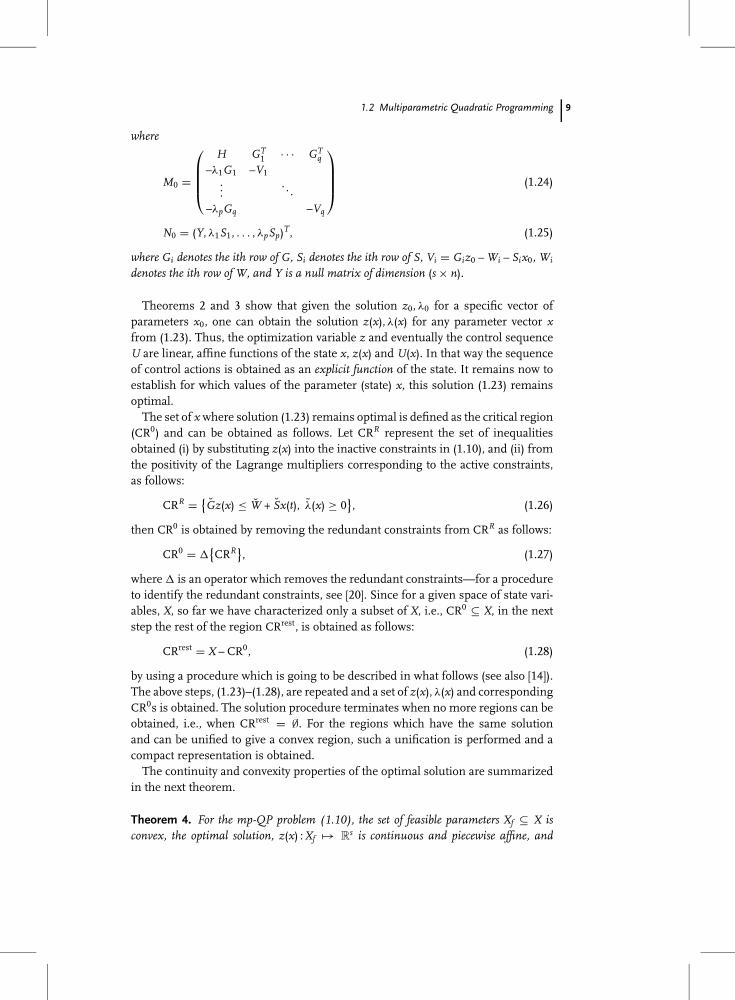
1.2 Multiparametric Quadratic Programming 9
where
M0 =
H GT1 · · · GT
q–λ1G1 –V1
.... . .
–λpGq –Vq
(1.24)
N0 = (Y, λ1S1, . . . , λpSp)T, (1.25)
where Gi denotes the ith row of G, Si denotes the ith row of S, Vi = Giz0 – Wi – Six0, Wi
denotes the ith row of W, and Y is a null matrix of dimension (s × n).
Theorems 2 and 3 show that given the solution z0, λ0 for a specific vector ofparameters x0, one can obtain the solution z(x), λ(x) for any parameter vector xfrom (1.23). Thus, the optimization variable z and eventually the control sequenceU are linear, affine functions of the state x, z(x) and U(x). In that way the sequenceof control actions is obtained as an explicit function of the state. It remains now toestablish for which values of the parameter (state) x, this solution (1.23) remainsoptimal.
The set of x where solution (1.23) remains optimal is defined as the critical region(CR0) and can be obtained as follows. Let CRR represent the set of inequalitiesobtained (i) by substituting z(x) into the inactive constraints in (1.10), and (ii) fromthe positivity of the Lagrange multipliers corresponding to the active constraints,as follows:
CRR = {Gz(x) ≤ W + Sx(t), λ(x) ≥ 0
}, (1.26)
then CR0 is obtained by removing the redundant constraints from CRR as follows:
CR0 = �{CRR}
, (1.27)
where � is an operator which removes the redundant constraints—for a procedureto identify the redundant constraints, see [20]. Since for a given space of state vari-ables, X, so far we have characterized only a subset of X, i.e., CR0 ⊆ X, in the nextstep the rest of the region CRrest, is obtained as follows:
CRrest = X – CR0, (1.28)
by using a procedure which is going to be described in what follows (see also [14]).The above steps, (1.23)–(1.28), are repeated and a set of z(x), λ(x) and correspondingCR0s is obtained. The solution procedure terminates when no more regions can beobtained, i.e., when CRrest = ∅. For the regions which have the same solutionand can be unified to give a convex region, such a unification is performed and acompact representation is obtained.
The continuity and convexity properties of the optimal solution are summarizedin the next theorem.
Theorem 4. For the mp-QP problem (1.10), the set of feasible parameters Xf ⊆ X isconvex, the optimal solution, z(x) : Xf → R
s is continuous and piecewise affine, and
10 1 Linear Model Predictive Control via Multiparametric Programming
the optimal objective function Vz(x) : Xf → R is continuous, convex, and piecewisequadratic.
Proof. We first prove convexity of Xf and Vz(x). Take generic x1, x2 ∈ Xf, and letVz(x1), Vz(x2), and z1, z2 be the corresponding optimal values and minimizers. Letα ∈ [0, 1], and define zα � αz1 + (1 – α)z2, xα � αx1 + (1 – α)x2. By feasibility, z1,z2 satisfy the constraints Gz1 ≤ W + Sx1, Gz2 ≤ W + Sx2. These inequalities canbe linearly combined to obtain Gzα ≤ W + Sxα , and therefore zα is feasible for theoptimization problem (1.10) where xt = xα . Since a feasible solution z(xα) exists atxα , an optimal solution exists at xα and hence Xf is convex. The optimal solution atxα will be less than or equal to the feasible solution, i.e.,
Vz(xα) ≤ 12
z′αHzα
and hence
Vz(xα) –12
[αz′
1Hz1 + (1 – α)z′2Hz2
]
≤ 12
z′αHzα –
12
[αz′
1Hz1 + (1 – α)z′2Hz2
]
= 12
[α2z′
1Hz1 + (1 – α)2z′2Hz2 + 2α(1 – α)z′
2Hz1 – αz′1Hz1 – (1 – α)z′
2Hz2]
= –12α(1 – α)(z1 – z2)′H(z1 – z2) ≤ 0, (1.29)
i.e.,
Vz(αx1 + (1 – α)x2
) ≤ αVz(x1) + (1 – α)Vz(x2)
∀x1, x2 ∈ X, ∀α ∈ [0, 1], which proves the convexity of Vz(x) on Xf. Within the closedpolyhedral regions CR0 in Xf the solution z(x) is affine (1.21). The boundary be-tween two regions belongs to both closed regions. Because the optimum is uniquethe solution must be continuous across the boundary. The fact that Vz(x) is contin-uous and piecewise quadratic follows trivially. �
An algorithm for the solution of an mp-QP of the form given in (1.10) to calculateU as an affine function of x and characterize X by a set of polyhedral regions, CRs, issummarized in Table 1.1. The optimal control sequence U*(x), once z(x) is obtainedby (1.23), is obtained from (1.9)
U*(x) = z(x) – H–1F′x. (1.30)
Finally, the feedback control law
ut = [I 0 · · · 0
]U*(xt) (1.31)
is applied to the system. The algorithm in Table 1.1 obtains the regions CR0s in thesubset X of the state space, where the optimal solution (1.23) and hence (1.31) exist.Hence, the MPC can be implemented by performing online the following heuristicrule:
1.2 Multiparametric Quadratic Programming 11
Table 1.1 mp-QP algorithm.
Step 1 For a given space of x solve (1.10) by treating x as a free variable and obtain [x0].Step 2 In (1.10) fix x = x0 and solve (1.10) to obtain [z0, λ0].Step 3 Obtain [z(x), λ(x)] from (1.23).Step 4 Define CRR as given in (1.26).Step 5 From CRR remove redundant inequalities and define the region of optimality CR0 as
given in (1.27).Step 6 Define the rest of the region, CRrest, as given in (1.28).Step 7 If no more regions to explore, go to the next step, otherwise go to Step 1.Step 8 Collect all the solutions and unify a convex combination of the regions having the
same solution to obtain a compact representation.
1. obtain the measurements of the state x at the current time;2. obtain the region CR0 in which x belongs, i.e., x ∈ CR0;3. obtain the control action ut from (1.31) and apply it to the
system;4. repeat in the next sampling instant.
Thus, the online optimization of the MPC problem (1.4) is reduced to the followingsimple function evaluation scheme:
if x ∈ CR0 then ut = [I 0 · · · 0
]U*(xt).
Remark 1. Note that the union of all regions CR0 forms the space of feasible parametersfor the mp-QP problem (1.10) which is also the space of feasible initial conditions forwhich a control exists that solves the MPC problem (1.4).
This approach provides a significant advancement in the solution and online im-plementation of MPC problems, since its application results in a complete set ofcontrol actions as a function of state variables (from (1.23)) and the correspondingregions of validity (from (1.27)), which are computed off-line, i.e., the explicit con-trol law. Therefore during online optimization, no optimizer call is required andinstead the region CR0 for the current state of the plant where the value of the statevariables is valid, can be identified by substituting the value of these state variablesinto the inequalities which define the regions. Then, the corresponding control ac-tions can be computed by using a function evaluation of the corresponding affinefunction.
1.2.1Definition of CRrest
This section describes a procedure for calculating the rest CRrest of a subset X,when a region of optimality CR0 ⊆ X is given, i.e., CRrest = X – CR0. For thesake of simplifying the explanation of the procedure, consider the case when only
12 1 Linear Model Predictive Control via Multiparametric Programming
Fig. 1.1 Critical regions, X and CR0.
two state-variables x1 and x2, are present (see Fig. 1.1), and X is defined by theinequalities:
X �{x ∈ R
n | xL1 ≤ x1 ≤ xU
1 , xL2 ≤ x2 ≤ xU
2}
and CR0 is defined by the inequalities:
CR0 � {x ∈ Rn | C1 ≤ 0, C2 ≤ 0, C3 ≤ 0},
where C1, C2, and C3 represent linear functions of x. The procedure consists ofconsidering one by one the inequalities which define CR0. Considering, for exam-ple, the inequality C1 ≤ 0, the rest of the region is given by
CRrest1 = {
x ∈ Rn | C1 ≥ 0, xL
1 ≤ x1, x2 ≤ xU2}
which is obtained by reversing the sign of inequality C1 ≤ 0 and removing redun-dant constraints in X (see Fig. 1.2). Thus, by considering the rest of the inequalities,the complete rest of the region is given by
CRrest = {CRrest
1 ∪ CRrest2 ∪ CRrest
3},
where CRrest1 , CRrest
2 , and CRrest3 are given in Table 1.2 and are graphically depicted
in Fig. 1.3. Note that for the case when X is unbounded, simply suppress the in-equalities involving X in Table 1.2.
Table 1.2 Definition of rest of the regions.
Region Inequalities
CRrest1 C1 ≥ 0, xL
1 ≤ x1, x2 ≤ xU2
CRrest2 C1 ≤ 0, C2 ≥ 0, x1 ≤ xU
1 , x2 ≤ xU2
CRrest3 C1 ≤ 0, C2 ≤ 0, C3 ≥ 0, xL
1 ≤ x1 ≤ xU1 , xL
2 ≤ x2
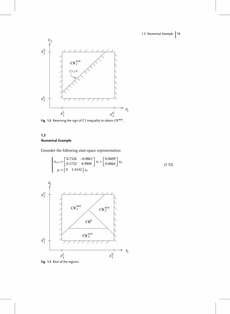
1.3 Numerical Example 13
Fig. 1.2 Reversing the sign of C1 inequality to obtain CRrest.
1.3Numerical Example
Consider the following state-space representation:
xt+1 =[
0.7326 –0.08610.1722 0.9909
]xt +
[0.06090.0064
]ut,
yt =[
0 1.4142]
xt.(1.32)
Fig. 1.3 Rest of the regions.
14 1 Linear Model Predictive Control via Multiparametric Programming
Fig. 1.4 Closed-loop response.
The constraints on input are as follows:
–2 ≤ ut ≤ 2. (1.33)
The corresponding optimization problem of the form (1.4) for regulating to theorigin is given as follows:
minut ,ut+1
x′t+2|tPxt+2|t +
1∑k=0
[x′
t+k|txt+k|t + 0.01u2t+k
]
s.t. –2 ≤ ut+k ≤ 2, k = 0, 1xt|t = xt,
(1.34)
where P solves the Lyapunov equation P = A′PA + Q,
Q =[
100 1
], R = 0.01, Nu = Ny = Nc = 2.
The closed-loop response from the initial condition x0 = [1 1]′ is shown in Fig. 1.4.The same problem is now solved by using the parametric programming approach.The corresponding mp-QP problem of the form (1.10) has the following constantvectors and matrices:
H =[
0.0196 0.00630.0063 0.0199
], F =
[0.1259 0.06790.0922 –0.0924
]
G =
1 0–1 00 10 –1
, W =
2222
, E =
y
0 00 00 00 0
.
The solution of the mp-QP problem, as computed by using the algorithm given inTable 1.1, is given in Table 1.3 and is depicted in Fig. 1.5. Note that the CRs 2, 4and 7, 8 in Table 1.3 are combined together and a compact convex representationis obtained. To illustrate how online optimization reduces to a function evaluation
1.3 Numerical Example 15
Fig. 1.5 Polyhedral partition of the state space.
Table 1.3 Parametric solution of the numerical example.
16 1 Linear Model Predictive Control via Multiparametric Programming
Fig. 1.6 Closed-loop response with additional constraint xt+k|t ≥ –0.5.
problem, consider the starting point x0 = [1 1]′. This point is substituted into theconstraints defining the CRs in Table 1.3 and it satisfies only the constraints ofCR7,8 (see also Fig. 1.5). The control action corresponding to CR7,8 from Table 1.3is u7,8 = –2, which is obtained without any further optimization calculations and itis same as the one obtained from the closed-loop response depicted in Fig. 1.4.
The same example is repeated with the additional constraint on the state
xt+k|t ≥ xmin, xmin �[
–0.5–0.5
], k = 1.
The closed-loop behavior from the initial condition x0 = [1 1]′ is presented inFig. 1.6. The MPC controller is given in Table 1.4. The polyhedral partition of thestate-space corresponding to the modified MPC controller is shown in Fig. 1.7. Thepartition consists now of 11 regions. Note that there are feasible states smaller thanxmin, and vice versa, infeasible states x ≥ xmin. This is not surprising. For instance,the initial state x0 = [–0.6 0]′ is feasible for the MPC controller (which checks stateconstraints at time t + k, k = 1), because there exists a feasible input such that x1
is within the limits. In contrast, for x0 = [–0.47 –0.47]′ no feasible input is ableto produce a feasible x1. Moreover, the union of the regions depicted in Fig. 1.7should not be confused with the region of attraction of the MPC closed loop. Forinstance, by starting at x0 = [46.0829 –7.0175]′ (for which a feasible solution exists),the MPC controller runs into infeasibility after t = 9 time steps.
1.4Computational Complexity
The algorithm given in Table 1.1 solves an mp-QP by partitioning X in Nr convexpolyhedral regions. This number Nr depends on the dimension n of the state, the
1.4 Computational Complexity 17
Fig. 1.7 Polyhedral partition of the state space with additional constraint xt+k|t ≥ –0.5.
product s = mNu of the number Nu of control moves and the dimension m of theinput vector, and the number of constraints q in the optimization problem (1.10).
In an LP the optimum is reached at a vertex, and therefore s constraints mustbe active. In a QP the optimizer can lie everywhere in the admissible set. As thenumber of combinations of � constraints out of a set of q is(
q�
)= q!
(q – �)!�!(1.35)
the number of possible combinations of active constraints at the solution of a QPis at most
q∑�=0
(q�
)= 2q. (1.36)
This number represents an upper bound on the number of different linear feed-back gains which describe the controller. In practice, far fewer combinations areusually generated as x spans X. Furthermore, the gains for the future input movesut+1, . . . , ut+Nu–1 are not relevant for the control law. Thus several different combi-nations of active constraints may lead to the same first m components u*
t (x) of thesolution. On the other hand, the number Nr of regions of the piecewise affine so-lution is in general larger than the number of feedback gains, because the regionshave to be convex sets.
A worst case estimate of Nr can be computed from the way the algorithm in Ta-ble 1.1 generates critical regions CR to explore the set of parameters X. The follow-ing analysis does not take into account (i) the reduction of redundant constraints,and (ii) possible empty sets are not further partitioned. The first critical region CR0
is defined by the constraints λ(x) ≥ 0 (q constraints) and Gz(x) ≤ W + Sx (q con-straints). If the strict complementary slackness condition holds, only q constraintscan be active, and hence CR is defined by q constraints. From Section 1.2.1, CRrest
consists of q convex polyhedra CRi, defined by at most q inequalities. For each CRi,
18 1 Linear Model Predictive Control via Multiparametric Programming
Table 1.4 Parametric solution of the numerical example for xt+k|t ≥ –0.5.
a new CR is determined which consists of 2q inequalities (the additional q inequal-ities come from the condition CR ⊆ CRi), and therefore the corresponding CRrest
partition includes 2q sets defined by 2q inequalities. As mentioned above, this wayof generating regions can be associated with a search tree. By induction, it is easy toprove that at the tree level k+1 there are k!mk regions defined by (k+1)q constraints.As observed earlier, each CR is the largest set corresponding to a certain combina-
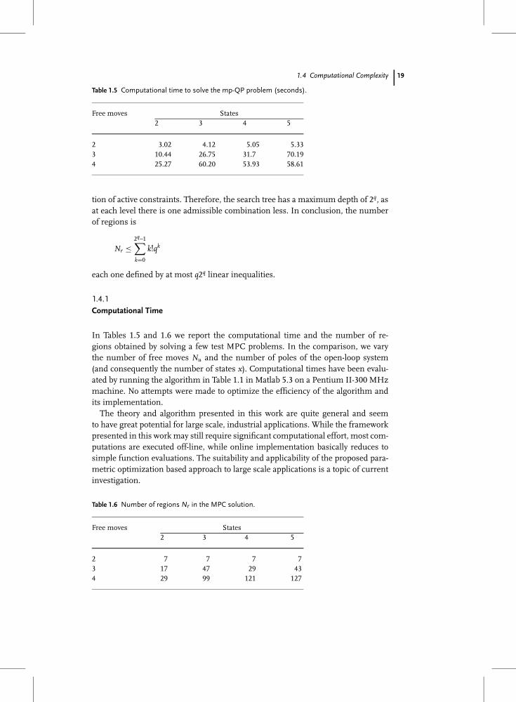
1.4 Computational Complexity 19
Table 1.5 Computational time to solve the mp-QP problem (seconds).
tion of active constraints. Therefore, the search tree has a maximum depth of 2q, asat each level there is one admissible combination less. In conclusion, the numberof regions is
Nr ≤2q–1∑k=0
k!qk
each one defined by at most q2q linear inequalities.
1.4.1Computational Time
In Tables 1.5 and 1.6 we report the computational time and the number of re-gions obtained by solving a few test MPC problems. In the comparison, we varythe number of free moves Nu and the number of poles of the open-loop system(and consequently the number of states x). Computational times have been evalu-ated by running the algorithm in Table 1.1 in Matlab 5.3 on a Pentium II-300 MHzmachine. No attempts were made to optimize the efficiency of the algorithm andits implementation.
The theory and algorithm presented in this work are quite general and seemto have great potential for large scale, industrial applications. While the frameworkpresented in this work may still require significant computational effort, most com-putations are executed off-line, while online implementation basically reduces tosimple function evaluations. The suitability and applicability of the proposed para-metric optimization based approach to large scale applications is a topic of currentinvestigation.
Table 1.6 Number of regions Nr in the MPC solution.
Free moves States2 3 4 5
2 7 7 7 73 17 47 29 434 29 99 121 127
20 1 Linear Model Predictive Control via Multiparametric Programming
1.5Extensions to the Basic MPC Problem
The basic MPC problem (1.4) and the corresponding mp-QP formulation (1.10),despite the fact that they treat the constrained regulation problem, can be extendedto treat other important control problems. To present the capability of multipara-metric programming to deal with a number of control problems, some of theseextensions are presented here.
1.5.1Reference Tracking
In reference tracking problems the objective is that the output, instead of beingregulated to the origin, is required to either asymptotically converge to a constantreference value or follow a reference signal that may vary in time. In either case, theobjective is to minimize the error between the system output yt and the referencesignal rt ∈ R
p, which is given by the problem specifications and is a function oftime.
The general MPC formulation to treat the reference tracking problem is
minU
J(U, xt, rt) =Ny–1∑k=0
(yt+k|t – rt
)′Q(yt+k|t – rt+k
)+ δu′
t+kRδut+k
s.t. ymin ≤ yt+k|t ≤ ymax, k = 1, . . . , Nc
umin ≤ ut+k ≤ umax, k = 0, 1, . . . , Nc
δumin ≤ δut+k ≤ δumax, k = 0, 1, . . . , Nu – 1xt+k+1|t = Axt+k|t + But+k, k ≥ 0yt+k|t = Cxt+k|t, k ≥ 0ut+k = ut+k–1 + δut+k, k ≥ 0δut+k = 0, k ≥ Nu,
(1.37)
where U � {δut, . . . , δut+Nu–1}, rt � {rt, . . . , rt+Ny–1}, and δu ∈ Rm represent the
control increments that act as correcting terms in the input to force the output totrack the reference signal. The equation
ut+k = ut+k–1 + δut+k
corresponds to adding an integrator in the control loop. Due to this formulation,the past input ut–1 is introduced in the above problem as a new vector of m para-meters.
The reference tracking MPC (1.37) can be formulated into an mp-QP problem,just like the regulation problem (1.4), by using the same procedure described in(1.1) and (1.2). One should note, though, that the number of parameters in thiscase has increased since, except for the state x, the past input ut–1 and the referenceinputs rt were also introduced. Note, that if the reference is constant then rt = · · · =rt+Ny–1 = r and only one parameter, namely r, is introduced. By taking these extraparameters into account and repeating the procedure in Sections 1.1 and 1.2, wecan transform the tracking problem (1.37) into
1.5 Extensions to the Basic MPC Problem 21
J*(xt, ut–1, rt) = minU
{12
U′HU +[x′
tu′t–1r′
t]FU
}
s.t. GU ≤ W + E
xt
ut–1
r′t
(1.38)
and finally into the mp-QP problem
Vz(xt) = minz
12
z′Hz
s.t. Gz ≤ W + S
xt
ut–1
rt
,
(1.39)
where
z = U + H–1F′ xt
ut–1
rt
and S = E + GH–1F′.
The mp-QP algorithm (1.1) can then be used to solve (1.39). The solution of (1.39)U is a linear, piecewise affine function U(xt, ut–1, rt) of xt, ut–1, rt defined over a num-ber of regions CR0 where this solution is valid. The reference tracking MPC is im-plemented by applying the following control:
ut = ut–1 + δut(xt, ut–1, rt),
where δut(xt, ut–1, rt) is the first component of the vector U(xt, ut–1, rt).
1.5.2Relaxation of Constraints
It is rather inevitable in some applications to consider possible violation of the out-put and input constraints, which can lead to infeasible solution of the problem (1.4)[36]. It is a common practice then to relax some of the output constraints in order toguarantee that a feasible solution is obtained for (1.4) and that the input constraintsare satisfied, since usually these constraints are related to safety and performanceissues. Therefore, the output constraints have to be posed again as
ymin – εη ≤ yt ≤ ymax – εη,
where the scalar variable ε corresponds to the magnitude of the relaxation and thevector η ∈ R
p is constant and is used to determine the extent to which each of theconstraints is relaxed. In order to penalize the constraints violation the quadraticterm ε2 is added to the objective function and the relaxation variable ε is treatedas an optimization variable. Therefore, solving the mp-QP problem (1.10), with theextra optimization variable, ε is obtained as a piecewise affine function of the statewhich allows one to know the exact violation of the constraints for each value of thesystem states.
22 1 Linear Model Predictive Control via Multiparametric Programming
1.5.3The Constrained Linear Quadratic Regulator Problem
It is easy to observe that the MPC problem (1.4) describes the constrained linearquadratic (CLQR) problem [12, 32], when Nc = Nu = Ny = N and the state feedbackgain K and P are obtained from the solution of the unconstrained, infinite-horizonLQR problem (1.5). It is easy to note then that the solution to the CLQR, by follow-ing the mp-QP method described in Section 1.2, is obtained as a piecewise affinefunction of the states.
1.6Conclusions
The solution of the linear MPC optimization problem, with a quadratic objectiveand linear output and input constraints, by using multiparametric programmingtechniques and specifically multiparametric quadratic programming, provides acomplete map of the optimal control as a function of the states and the charac-teristic partitions of the state space where this solution is feasible. In that way thesolution of the MPC problem is obtained as piecewise affine feedback control law.The online computational effort is small since the online optimization problem issolved off-line and no optimizer is ever called online. In contrast, the online op-timization problem is reduced to a mere function evaluation problem; when themeasurements of the state are obtained and the corresponding region and controlaction are obtained by evaluation of a number of linear inequalities and a linearaffine function, respectively. This is known as the online optimization via off-lineparametric optimization concept.
References
1 Acevedo, J., Pistikopoulos, E. N., Ind.Eng. Chem. Res. 35 (1996), p. 147
2 Acevedo, J., Pistikopoulos, E. N., Ind.Eng. Chem. Res. 36 (1997), p. 2262
3 Acevedo, J., Pistikopoulos, E. N., Ind.Eng. Chem. Res. 36 (1997), p. 717
4 Acevedo, J., Pistikopoulos, E. N.,Oper. Res. Lett. 24 (1999), p. 139
5 Bansal, V., Perkins, J. D., Pis-
tikopoulos, E. N., AIChE J. 46(2000a), p. 335
6 Bansal, V., Perkins, J. D., Pis-
tikopoulos, E. N., J. Stat. Comput.Simul. 67 (2000b), pp. 219–253
7 Bemporad, A., Morari, M., Automat-ica 35 (1999), p. 407
8 Bemporad, A., Morari, M., in: Ro-bustness in Identification and Control,Lecture Notes in Control and Infor-mation Sciences, vol. 245, Springer,Berlin, 1999
9 Bemporad, A., Morari, M., Dua,
V., Pistikopoulos, E. N., Tech. Rep.AUT99-16, Automatic Control Lab,ETH Zürich, Switzerland, 1999
10 Bemporad, A., Morari, M., Dua, V.,
Pistikopoulos, E. N., Automatica 38(2002), p. 3
11 Chisci, L., Zappa, G., Int. J. Control 72(1999), p. 1020
References 23
12 Chmielewski, D., Manousiouthakis,
V., Syst. Control Lett. 29 (1996), p. 121
13 Dua, V., Pistikopoulos, E. N., Trans.IChemE 76 (1998), p. 408
14 Dua, V., Pistikopoulos, E. N., Ann.Oper. Res. 99 (1999), p. 123
15 Dua, V., Pistikopoulos, E. N., Ind.Eng. Chem. Res. 38 (1999), p. 3976
16 Edgar, T. F., Himmelblau, D. M., Op-timization at Chemical, McGraw-Hill,Singapore, 1989
23 Marlin, T. E., Hrymak, A. N., in: 5thInt. Conf. Chem. Proc. Control, AIChESymposium Series, vol. 93, 1997
24 Mayne, D. Q., Rawlings, J. B., Rao, C.
V., Scokaert, P. O. M., Automatica 36(2000), p. 789
25 Morari, M., Lee, J., Comput. Chem.Eng. 23 (1999), p. 667
26 Papalexandri, K., Dimkou, T. I., Ind.Eng. Chem. Res. 37 (1998), p. 1866
27 Pertsinidis, A., On the parametricoptimization of mathematical pro-grams with binary variables and itsapplication in the chemical engineer-ing process synthesis, Ph.D. Thesis,Carnegie Mellon University, Pittsburg,PA, USA, 1992
28 Pertsinidis, A., Grossmann, I. E.,
McRae, G. J., Comput. Chem. Eng. 22(1998), p. S205.
29 Pistikopoulos, E. N., Dua, V., in: Proc.3rd Int. Conf. on FOCAPO, 1998
30 Pistikopoulos, E. N., Grossmann,
I. E., Comput. Chem. Eng. 12 (1988),p. 719
31 Pistikopoulos, E. N., Dua, V., Bozi-
nis, N. A., Bemporad, A., Morari, M.,Comput. Chem. Eng. 26 (2002), p. 175