40
1 Mapping the State of Financial Stability 14th Annual DNB Research Conference 3rd November 2011 DNB, Amsterdam Peter Sarlin (Åbo Akademi / TUCS) & Tuomas Peltonen (European Central Bank)
| Date post: | 30-Dec-2015 |
| Category: |
Documents |
| Upload: | ellen-chapman |
| View: | 219 times |
| Download: | 0 times |

1
Mapping the State of Financial Stability
14th Annual DNB Research Conference3rd November 2011
DNB, Amsterdam
Peter Sarlin (Åbo Akademi / TUCS) &Tuomas Peltonen (European Central Bank)

2
An example of a SOM output at certain timeAn example of a SOM output at certain time
Taiwan
India
UK Indonesia
Japan Thailand
Canada
Russia Czech Republic
Poland Norway
Hungary
China Hong Kong Switzerland
Australia New Zealand
US
Denmark Euro area
Korea Sweden
Argentina Brazil
Mexico Turkey
Malaysia Philippines
Singapore South Africa
Crisis
Post crisis
Tranquil
Pre crisis

3
1. Introduction - motivation1. Introduction - motivation
Global Financial Stability Map (GFSM)
IMF GFSR September 2011 (Dattels et al., 2010)
• Current state-of-the-Current state-of-the-art: Six composite art: Six composite indices describing indices describing the state of financial the state of financial stability (area) and stability (area) and various aspects of various aspects of vulnerabilities vulnerabilities (dimensions)…(dimensions)…

4
• ... ... fall short in fall short in disentangling disentangling the the sources of sources of vulnerabilityvulnerability as as further indicatorsfurther indicators are are needed.needed.
• IMF/Dattels et al. IMF/Dattels et al. (2010) use market (2010) use market intelligence and other intelligence and other types of technical types of technical adjustments to GFSM adjustments to GFSM for describing the for describing the vulnerabilitiesvulnerabilities
• ➨➨ no attempt to no attempt to measure the precision measure the precision of of out-of-sampleout-of-sample prediction of systemic prediction of systemic events. events. ➨➨What does a What does a certain level of certain level of vulnerabilities wrt. vulnerabilities wrt. future crisis? future crisis?
1. Introduction - motivation1. Introduction - motivation

5
1. Introduction - motivation1. Introduction - motivation
• Common limitations Common limitations of spider charts: The of spider charts: The area does not scale 1-area does not scale 1-to-1 with increases in to-1 with increases in vulnerabilities and vulnerabilities and depends on the order depends on the order of dimensionsof dimensions
• In the charts (e.g. In the charts (e.g. two different two different countries), the only countries), the only actual difference in actual difference in the aggregate degree the aggregate degree of vulnerability is the of vulnerability is the dimensions and their dimensions and their orderorder
Emerging market risks
Credit risks
Market and liquidity risks
Risk apetite
Monetary and financial
Macroeconomic risks
Emerging market risks
Credit risks
Market and liquidity risks
Risk apetite
Monetary and financial
Macroeconomic risks

6
1. Introduction - 1. Introduction - What do we do in the paper?What do we do in the paper?
• Create the Create the Self-Organizing Financial Stability Map Self-Organizing Financial Stability Map (SOFSM)(SOFSM)
• A model that can A model that can visualize multidimensional visualize multidimensional macro-financial vulnerabilities and the state of macro-financial vulnerabilities and the state of financial stability financial stability across countries and over across countries and over timetime
• A model that has A model that has good out-of-sample predictive good out-of-sample predictive capabilities of future capabilities of future systemic events systemic events / financial / financial crisescrises

7
2. Self-Organizing Financial Stability Map (SOFSM)2. Self-Organizing Financial Stability Map (SOFSM)
• Building blocks for creating the SOFSM:Building blocks for creating the SOFSM:• Self-Organizing MapsSelf-Organizing Maps• Identifying systemic eventsIdentifying systemic events• Vulnerability indicatorsVulnerability indicators• Model training Model training • Model evaluationModel evaluation
• Mapping the State of Financial StabilityMapping the State of Financial Stability
8
2.1 Self-Organizing Maps (SOMs)2.1 Self-Organizing Maps (SOMs) – – what are they? what are they?
• SOMSOM is an is an Exploratory Data AnalysisExploratory Data Analysis (EDA) technique (EDA) technique
by Kohonen (1981) ➨ Viscovery SOMineby Kohonen (1981) ➨ Viscovery SOMine• It is a It is a clusteringclustering and and projectionprojection technique: technique:
– Spatially constrained form of Spatially constrained form of kk-means clustering-means clustering– Preserves the Preserves the neighbourhood relations of the data neighbourhood relations of the data
(instead of trying to preserve the distances between data)(instead of trying to preserve the distances between data)– Projects data onto a grid of nodesProjects data onto a grid of nodes (rather than projecting (rather than projecting
data into a continuous space)data into a continuous space)
• Enables visualization of Enables visualization of high-D datahigh-D data ➨ ➨ 2D grid2D grid of of nodes without losing the topological relationships of nodes without losing the topological relationships of data and sight of individual indicators. data and sight of individual indicators.
• Enables a Enables a flexible distribution and interactions.flexible distribution and interactions.• Kohonen’s group has continuously reviewed the SOM Kohonen’s group has continuously reviewed the SOM
literatureliterature• The SOM has been used in approx. 10 000 worksThe SOM has been used in approx. 10 000 works• Applied to currency and debt crises: Arciniegas and Applied to currency and debt crises: Arciniegas and
Arciniegas Rueda (2009), Resta (2009), Sarlin (2011) and Arciniegas Rueda (2009), Resta (2009), Sarlin (2011) and Sarlin and Marghescu (2011)Sarlin and Marghescu (2011)
9
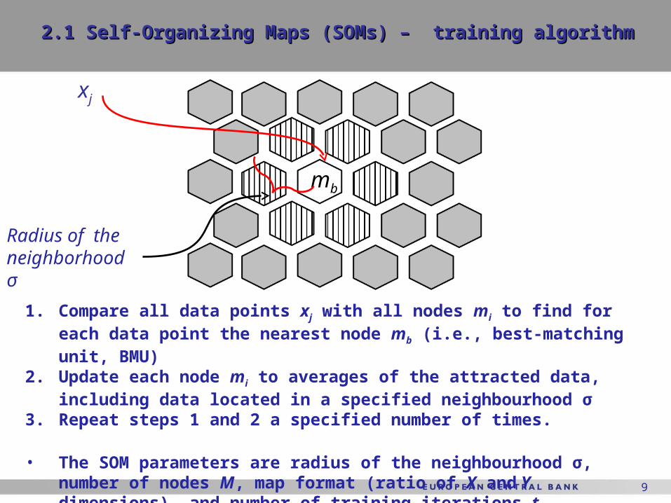
2.1 Self-Organizing Maps (SOMs)2.1 Self-Organizing Maps (SOMs) – – training algorithm training algorithm
mb
xj
Radius of the neighborhood σ
1. Compare all data points xj with all nodes mi to find for each data point the nearest node mb (i.e., best-matching unit, BMU)
2. Update each node mi to averages of the attracted data, including data located in a specified neighbourhood σ
3. Repeat steps 1 and 2 a specified number of times.
• The SOM parameters are radius of the neighbourhood σ, number of nodes M, map format (ratio of X and Y dimensions), and number of training iterations t.

10
2.1 Self-Organizing Maps (SOMs) –2.1 Self-Organizing Maps (SOMs) – interpreting the interpreting the outputoutput
• This is a This is a 2D map 2D map that that represents multi-D data with represents multi-D data with a 2-level clusteringa 2-level clustering
• For each indicator, we For each indicator, we create a create a „feature plane“ „feature plane“ where the color coding where the color coding represents the represents the distributiondistribution of its values on the 2D mapof its values on the 2D map..
Indicator 1Indicator 1 Indicator 2 Indicator 3 Indicator 2 Indicator 3 Indicator 4 Indicator 4

11
2.2 Identifying systemic events and creating financial 2.2 Identifying systemic events and creating financial stability cyclestability cycle
• Use the data set from Use the data set from Lo Duca and Peltonen (2011)Lo Duca and Peltonen (2011): : 28 28
countries (18 EMEs & 10 AEs), Quarterly data 1990Q1-countries (18 EMEs & 10 AEs), Quarterly data 1990Q1-2010Q32010Q3
• Identification of Identification of systemic eventssystemic events::• The The Financial Stress Index (FSI)Financial Stress Index (FSI) includes 5 components for includes 5 components for
each country, measuring volatilities and sharp declines in each country, measuring volatilities and sharp declines in key market segments (stock, foreign exchange and money key market segments (stock, foreign exchange and money markets)markets)
• A systemic event occurs when the FSI is above the 90A systemic event occurs when the FSI is above the 90thth percentile of the country-specific distribution (on average, percentile of the country-specific distribution (on average, negative real consequences)negative real consequences)
• Using the FSI, we identify four classes to describe the Using the FSI, we identify four classes to describe the financial stability cyclefinancial stability cycle::
• Pre-crisisPre-crisis periods (18 months before the systemic event) periods (18 months before the systemic event)• CrisisCrisis periods (systemic events defined by a financial periods (systemic events defined by a financial
stress index)stress index)• Post-crisisPost-crisis periods (18 months after the systemic event) periods (18 months after the systemic event)• Tranquil Tranquil periods (all other periods)periods (all other periods)

12
2.2. Financial Stress Index (FSI)2.2. Financial Stress Index (FSI)
• A simple Financial Stress Index(1) the spread of the 3-month interbank rate over the 3-month Government bill rate (Ind1)(2) negative quarterly equity returns (Ind2) (3) the realized volatility of the main equity index (as average daily absolute changes over a quarter) (Ind3) (4) the realized volatility of the nominal effective exchange rate (Ind4) (5) the realized volatility of the yield on the 3-month Government bill (Ind5).
• Each component j of the index for country i at quarter t is transformed into an integer that ranges from 0 to 3 according to the country-specific quartile of the distribution:
5
)(5
1,,,,
,
j
tijtij
ti
Indq
FSI
13
2.3 Vulnerability indicators2.3 Vulnerability indicators
• 14 indicators of country-level 14 indicators of country-level macro-financial macro-financial vulnerabilitiesvulnerabilities::
• DomesticDomestic = inflation, GDP growth, CA deficit, budget = inflation, GDP growth, CA deficit, budget balance, credit growth, leverage, equity price growth, balance, credit growth, leverage, equity price growth, equity valuationequity valuation
• GlobalGlobal = = inflation, GDP growth, credit growth, inflation, GDP growth, credit growth, leverage, equity price growth, equity valuationleverage, equity price growth, equity valuation
• Test several Test several transformationstransformations of the indicators (over 200 of the indicators (over 200 transformations of the indicators tested). transformations of the indicators tested).
• Select best-performing (as a leading indicator) Select best-performing (as a leading indicator) transformations of the variablestransformations of the variables

14
2.4 Model training2.4 Model training
• „„Static“ modelStatic“ model, i.e. model is not re-, i.e. model is not re-
estimated recursively:estimated recursively:• Training set (estimation sample): 1990Q4 - Training set (estimation sample): 1990Q4 -
2005Q12005Q1• Test set (out-of-sample): 2005Q2 - 2009Q2Test set (out-of-sample): 2005Q2 - 2009Q2• In the benchmark, we use 18 months as a In the benchmark, we use 18 months as a
forecast horizonforecast horizon• Account for policymakers’ preferences Account for policymakers’ preferences
when evaluating the performance as in when evaluating the performance as in Alessi and Detken (2011) (benchmark Alessi and Detken (2011) (benchmark μμ=0.5=0.5) )
• Data as anData as an input to the SOFSMinput to the SOFSM• Class variables + vulnerabilities for Class variables + vulnerabilities for
trainingtraining• Only vulnerabilities for mapping and Only vulnerabilities for mapping and
evaluatingevaluating
• Crisis probabilities as an output of Crisis probabilities as an output of the SOFSMthe SOFSM
• Map data onto SOFSM and retrieve a crisis Map data onto SOFSM and retrieve a crisis probabilityprobability
Crisis
TranquilPre crisis
Post crisis
Euro area
C18
Crisis
TranquilPre crisis
Post crisis
Euro area
0.01 0.10 0.19 0.28 0.38 0.47 0.56 0.65

15
2.5 Model evaluation2.5 Model evaluation
• Evaluate output using the „Evaluate output using the „usefulnessusefulness“ criterion (see e.g. “ criterion (see e.g. Alessi and Detken (2011)) and compare it with a Lo Duca and Alessi and Detken (2011)) and compare it with a Lo Duca and Peltonen (2011)-type Peltonen (2011)-type logitlogit model model
• Find the threshold that Find the threshold that minimizes a loss function that depends that depends on policymaker’ preferences between on policymaker’ preferences between type I and type II errors
• DefineDefine Usefulness “U”
• In the benchmark model, we set In the benchmark model, we set µµ = = 0.5, i.e. we assume the i.e. we assume the policymaker ispolicymaker is equally concerned of missing systemic events and issuing false alarms (“neutral external observer”)(“neutral external observer”)
))/()(1())/(()( TNFPFPTPFNFNL
)(1,Min LU
Actual class
Systemic event within a given time horizon
No systemic event within a given time horizon
1 -1
Predicted class
Indicator above threshold (Signal)
1
True positive (TP) (correct signals)
False positive (FP) (wrong signals)
Indicator below threshold (No signal)
-1
False negative (FN) (missing signals)
True negative (TN) (correct absence of signals)

16
2.5 Model evaluation2.5 Model evaluation
• Defining early warning nodesDefining early warning nodes• When calibrating the policymakers’ preferences, we When calibrating the policymakers’ preferences, we
vary the thresholds. This changes the number of “early vary the thresholds. This changes the number of “early warning nodes”.warning nodes”.
µ µ =0.4=0.4 µ µ =0.5=0.5 µ µ =0.6=0.6

17
Data set μ Precision Recall Precision Recall AUCLogit Train 0.5 162 190 830 73 0.46 0.69 0.92 0.81 0.79 0.25 0.81SOM Train 0.5 190 314 706 45 0.38 0.81 0.94 0.69 0.71 0.25 0.83
Logit Test 0.5 77 57 249 93 0.57 0.45 0.73 0.81 0.68 0.13 0.72SOM Test 0.5 112 89 217 58 0.56 0.66 0.79 0.71 0.69 0.18 0.75
Tranquil periods
Accuracy UModel TP FP TN FN
Crash periods
2.5 Model evaluation2.5 Model evaluation
• Training the SOM:Training the SOM:• While a higher number of nodes While a higher number of nodes M M improves in-sample improves in-sample performance, it decreases generalization, i.e. out-of-sample performance, it decreases generalization, i.e. out-of-sample performance.performance.• We increase We increase MM and find and find the first model with Usefulness ≥ 0.25 the first model with Usefulness ≥ 0.25 (logit model).(logit model).
• In terms of “In terms of “UsefulnessUsefulness”, when ”, when µµ=0.5, the models are by =0.5, the models are by definition very similar on in-sample data, while the SOM performs definition very similar on in-sample data, while the SOM performs better on out-of-sample data better on out-of-sample data • Robustness is tested with respect to three aspectsRobustness is tested with respect to three aspects
• SOM parameters: radius of neighborhood and number of SOM parameters: radius of neighborhood and number of nodesnodes• Policymakers’ preferencesPolicymakers’ preferences• Forecast horizonForecast horizon
The SOM detects more crises but issues also more ‘false’ warningsReminder:Recall positives = TP/(TP+FN), Recall negatives = TN/(TN+FP), Precision positives = TP/(TP+FP), Precision negatives = TN/(TN+FN), FP rate = FP/(FP+TN), TP rate = TP/(FN+ TP), Accuracy=(TP+TN)/(FN+FP+TN+ TP).
18
Crisis
TranquilPre crisis
Post crisis
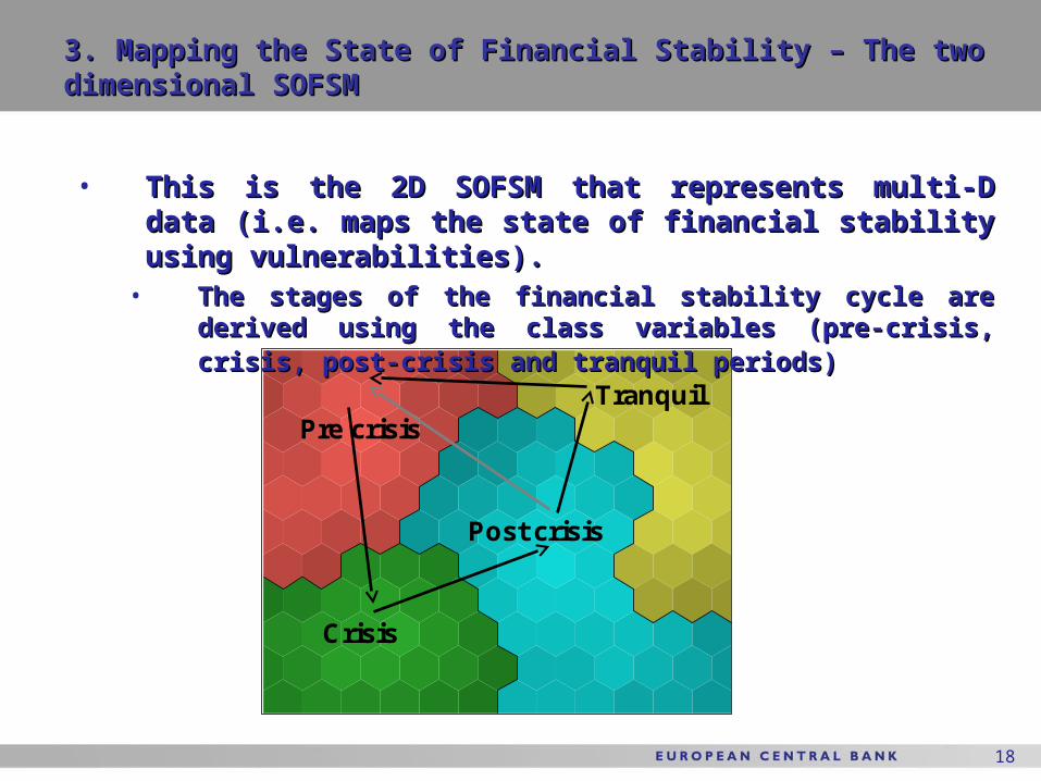
3. Mapping the State of Financial Stability – The two 3. Mapping the State of Financial Stability – The two dimensional SOFSMdimensional SOFSM
• This is the 2D SOFSM that represents multi-D data This is the 2D SOFSM that represents multi-D data (i.e. maps the state of financial stability using (i.e. maps the state of financial stability using vulnerabilities).vulnerabilities).
• The stages of the financial stability cycle are derived The stages of the financial stability cycle are derived using the class variables (pre-crisis, crisis, post-crisis using the class variables (pre-crisis, crisis, post-crisis and tranquil periods)and tranquil periods)

19
C24
Pre crisisTranquil
Crisis
Post crisis
0.01 0.26 0.50 0.75
C18
Pre crisisTranquil
Crisis
Post crisis
0.01 0.22 0.44 0.65
C12
Pre crisisTranquil
Crisis
Post crisis
0.00 0.18 0.35 0.53
C6
Pre crisisTranquil
Crisis
Post crisis
0.00 0.11 0.21 0.32
C0
Pre crisisTranquil
Crisis
Post crisis
0.00 0.23 0.47 0.70
P6
Pre crisisTranquil
Crisis
Post crisis
0.00 0.11 0.22 0.33
P12
Pre crisisTranquil
Crisis
Post crisis
0.01 0.18 0.35 0.52
P18
Pre crisisTranquil
Crisis
Post crisis
0.06 0.25 0.44 0.63
P24
Pre crisisTranquil
Crisis
Post crisis
0.13 0.32 0.50 0.68
T0
Pre crisisTranquil
Crisis
Post crisis
0.02 0.29 0.55 0.82
PPC0
Pre crisisTranquil
Crisis
Post crisis
0.00 0.09 0.18 0.27
3. Mapping the State of Financial Stability – Constructing 3. Mapping the State of Financial Stability – Constructing the four clusters according to the financial stability cyclethe four clusters according to the financial stability cycle
• Clustering is performed using Clustering is performed using hierarchical clustering hierarchical clustering based on based on class variables. class variables. The map is partitioned into four clusters The map is partitioned into four clusters according to the according to the financial stability cycle:financial stability cycle: a pre-crisis, crisis, a pre-crisis, crisis, post-crisis and tranquil cluster.post-crisis and tranquil cluster.
Co-occurrence of pre- and post-crisis
20
Inflation
Pre crisis
Crisis
Post crisis
Tranquil
0.17 0.29 0.41 0.52 0.64 0.76
Real GDP growth
Pre crisis
Crisis
Post crisis
Tranquil
0.14 0.27 0.41 0.55 0.69 0.83
Real credit growth
Pre crisis
Crisis
Post crisis
Tranquil
0.18 0.32 0.45 0.58 0.71 0.85
CA deficit
Pre crisis
Crisis
Post crisis
Tranquil
0.19 0.31 0.43 0.55 0.68 0.80
Government deficit
Pre crisis
Crisis
Post crisis
Tranquil
0.19 0.32 0.46 0.59 0.72 0.86
Global inflation
Pre crisis
Crisis
Post crisis
Tranquil
0.08 0.25 0.41 0.57 0.73 0.90
Global leverage
Pre crisis
Crisis
Post crisis
Tranquil
0.16 0.31 0.46 0.61 0.76 0.91
Global equity valuation
Pre crisis
Crisis
Post crisis
Tranquil
0.14 0.30 0.45 0.60 0.75 0.91
Pre-crisis periods
Pre crisis
Crisis
Post crisis
Tranquil
0.01 0.14 0.27 0.39 0.52 0.65
Real equity growth
Pre crisis
Crisis
Post crisis
Tranquil
0.16 0.30 0.43 0.57 0.71 0.85
Leverage
Pre crisis
Crisis
Post crisis
Tranquil
0.18 0.31 0.44 0.57 0.70 0.83
Equity valuation
Pre crisis
Crisis
Post crisis
Tranquil
0.17 0.30 0.43 0.55 0.68 0.81
Global real GDP growth
Pre crisis
Crisis
Post crisis
Tranquil
0.13 0.28 0.42 0.57 0.71 0.86
Global real credit growth
Pre crisis
Crisis
Post crisis
Tranquil
0.15 0.31 0.46 0.61 0.76 0.92
Global real equity growth
Pre crisis
Crisis
Post crisis
Tranquil
0.11 0.25 0.39 0.52 0.66 0.80
Crisis periods
Pre crisis
Crisis
Post crisis
Tranquil
0.00 0.14 0.28 0.42 0.56 0.70
Post-crisis periods
Pre crisis
Crisis
Post crisis
Tranquil
0.06 0.18 0.29 0.40 0.52 0.63
Tranquil periods
Pre crisis
Crisis
Post crisis
Tranquil
0.02 0.18 0.34 0.50 0.66 0.82
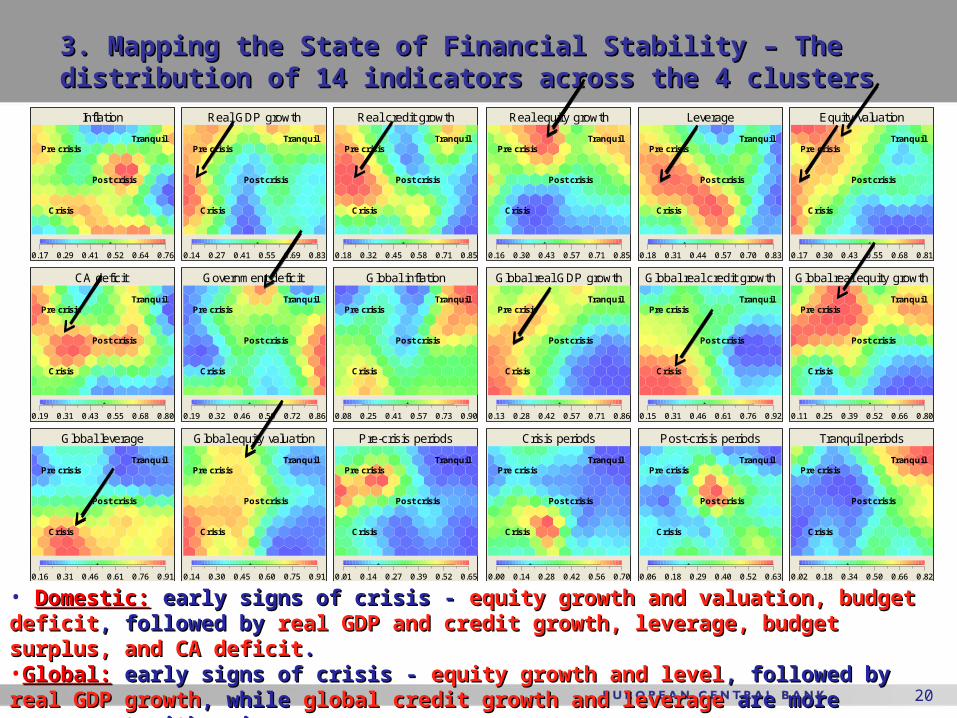
3. Mapping the State of Financial Stability – The 3. Mapping the State of Financial Stability – The distribution of 14 indicators across the 4 clustersdistribution of 14 indicators across the 4 clusters
• Domestic:Domestic: early signs of crisis - early signs of crisis - equity growth and valuation, budget deficitequity growth and valuation, budget deficit, , followed by followed by real GDP and credit growth, leverage, budget surplus, and CA real GDP and credit growth, leverage, budget surplus, and CA deficitdeficit. . •Global:Global: early signs of crisis - early signs of crisis - equity growth and levelequity growth and level, followed by , followed by real GDPreal GDP growthgrowth, while , while global credit growth and leverage global credit growth and leverage are more concurrent with are more concurrent with crises.crises.

21
3. Mapping the State of Financial Stability – Temporal 3. Mapping the State of Financial Stability – Temporal dimensiondimension
Evolution of macro-financial conditions (all 14 indicators) for the United States and the Euro area (2002-10, first quarter)
In 2010Q1, the euro area aggregate, did not reflect the crisis in GR, IE, PT.
Financial Stress Index also decreased for the euro area aggregate in 2010Q1
Crisis
TranquilPre crisis
Post crisis
US20022010
US2008–09
US2007
US2006
US2004–05
US2003
Euro2002
Euro2003
Euro2004–05
Euro2006
Euro2007
Euro2008
Euro2009
Euro2010

22
Taiwan
India
UK Indonesia
Japan Thailand
Canada
Russia Czech Republic
Poland Norway
Hungary
China Hong Kong Switzerland
Australia New Zealand
US
Denmark Euro area
Korea Sweden
Argentina Brazil
Mexico Turkey
Malaysia Philippines
Singapore South Africa
Crisis
Post crisis
Tranquil
Pre crisis
3. Mapping the State of Financial Stability – Cross section3. Mapping the State of Financial Stability – Cross section
Visualizing current macro-financial vulnerabilities in key advanced and emerging economies (2010Q3)
Contagion through similarities in macro-financial vulnerabilities

23
3. Mapping the State of Financial Stability – Regional 3. Mapping the State of Financial Stability – Regional evolutionevolution
Evolution of the macro-financial conditions in Emerging Market Economies and Advanced Economies (2002-10 , first quarter)
Pre-crisis
Crisis
Post-crisis
Tranquil
Crisis
Pre crisis
Post crisis
EME 2005
AE 2004
EME 2004 AE
2005
AE 2006
AE 2010
AE 2007
EME 2010
AE 2002
EME 2002
EME 2008
AE 2008
AE 2003
EME 2003
EME 2006 2007
Tranquil
AE 2009
EME 2009
24
4. Conclusions4. Conclusions
• Self-Organizing Financial Stability Map Self-Organizing Financial Stability Map is a useful is a useful model for financial stability surveillance:model for financial stability surveillance:
• mapping the state of financial stability mapping the state of financial stability and and visualizing multidimensional macro-financial visualizing multidimensional macro-financial vulnerabilitiesvulnerabilities
• has has good out-of-sample predictive good out-of-sample predictive capabilities capabilities of future of future systemic events systemic events / financial crises / financial crises (EWS)(EWS)
• the SOFSM is flexible with respect to, e.g., the SOFSM is flexible with respect to, e.g., events of interest, vulnerability indicators, events of interest, vulnerability indicators, forecast horizons, policymaker‘s preferencesforecast horizons, policymaker‘s preferences

25
Thank you for your attention!Thank you for your attention!

26
Extra slidesExtra slides

27
2. Self-Organizing Maps (SOMs)2. Self-Organizing Maps (SOMs) – – Kohonen training Kohonen training algorithmalgorithm
1. Initialization using the two principal components1. Initialization using the two principal components
2. Finding the best-matching units2. Finding the best-matching units
where each data point where each data point xx is matched with its BMU is matched with its BMU mmcc..
3. Update the reference vectors (or units or nodes)3. Update the reference vectors (or units or nodes)
where the neighborhood where the neighborhood h h is given byis given by
where r is the 2D coordinates of where r is the 2D coordinates of mmcc and and mmii and is a specified tension and is a specified tension
value.value.
4. Cluster the units using Ward4. Cluster the units using Ward’’s hierarchical s hierarchical clusteringclustering
ii
c mxmx min
,)(
)(
)1(
1)(
1)(
N
jjic
N
jjjic
i
th
xth
tm
,)(2
exp2
2
)(
t
rrh ic
jic
)(t

28
Descriptive statistics of the dataDescriptive statistics of the data
Type Variable Abbreviation Mean SD Min. Max. Skew. Kurt. KSL ADDomestic Inflation
aInflation 0.89 5.17 -10.15 42.53 4.80 26.72 0.29* 263.90*
Domestic Real GDPb
Real GDP growth 3.73 3.76 -17.54 14.13 -0.86 3.16 0.06* 11.34*Domestic Real credit to private sector to GDP
bReal credit growth 234.07 4724.00 -69.42 101870.34 20.76 429.59 0.51* Inf*
Domestic Real equity pricesb
Real equity growth 5.93 33.01 -84.40 257.04 0.99 4.31 0.05* 7.28*Domestic Credit to private sector to GDP
aLeverage 3.48 51.64 -62.78 1673.04 22.76 673.35 0.29* Inf*
Domestic Stock market capitalisation to GDPa
Equity valuation 3.90 28.32 -62.79 201.55 0.77 2.41 0.03* 3.86*Domestic Current account deficit to GDP
cCA deficit -0.02 0.07 -0.27 0.10 -0.98 0.73 0.09* 33.12*
Domestic Government deficit to GDPc
Government deficit 0.01 0.05 -0.19 0.22 -1.09 3.46 0.09* 35.90*
Global Inflationa
Global inflation 0.03 0.64 -1.33 2.29 0.71 1.28 0.08* 12.12*Global Real GDP
bGlobal real GDP growth 1.84 1.59 -6.34 4.09 -3.02 11.74 0.20* 122.16*
Global Real credit to private sector to GDPb
Global real credit growth 3.87 1.68 -0.23 7.20 -0.21 -0.31 0.07* 8.82*Global Real equity prices
bGlobal real equity growth 2.31 19.08 -40.62 37.77 -0.57 -0.68 0.15* 41.90*
Global Credit to private sector to GDPa
Global leverage 1.15 2.79 -2.79 11.21 1.84 3.40 0.22* 105.26*Global Stock market capitalisation to GDP
aGlobal equity valuation 0.89 17.41 -40.54 27.46 -0.50 -0.43 0.09* 19.11*
Notes: Transformations: a, deviation from trend; b, annual change; c, level. KSL: Lilliefors' adaption of the Kolmogorov-Smirnov normality test. AD: the standard Anderson-Darling normality test. Significance levels: 1%, *.

29
The logit modelThe logit model
Variable EstimateStd.
Error Z
Intercept -6.744 0.612 -11.024 0.000 ***Inflation -0.100 0.300 -0.334 0.738Real GDP growth 0.076 0.334 0.229 0.819Real credit growth -0.001 0.001 -0.613 0.540Real equity growth 1.791 0.382 4.685 0.000 ***Leverage 0.003 0.001 3.204 0.001 ***Equity valuation 0.002 0.001 2.689 0.007 ***CA deficit 1.151 0.308 3.741 0.000 ***Government deficit 0.076 0.342 0.223 0.823
Global inflation 0.207 0.341 0.608 0.543Global real GDP growth 1.156 0.419 2.761 0.006 ***Global real credit growth 0.685 0.381 1.799 0.072 *Global real equity growth 0.832 0.419 1.985 0.047 **Global leverage 0.712 0.427 1.668 0.095 *Global equity valuation 0.959 0.472 2.029 0.042 **
Sig.
Notes: Significance levels: 1%, ***; 5 %, **; 10 %, *.
30
Evaluation measuresEvaluation measures
• Recall positives(RP) = TP/(TP+FN), • Recall negatives(RN) = TN/(TN+FP)• Precision positives(PP) = TP/(TP+FP)• Precision negatives(PN) = TN/(TN+FN)• Overall accuracy = (TP+TN)/(TP+TN+FP+FN),• FP rate = FP/(FP+TN) • FN rate = FN/(FN+ TP)•ROC curve = TP rate vs. FP rate •AUC = Area under the ROC curve (probability that a randomly chosen positive instance is ranked higher than a randomly chosen negative instance)
Actual class
Systemic event within a given time horizon
No systemic event within a given time horizon
1 -1
Predicted class
Indicator above threshold (Signal)
1
True positive (TP) (correct signals)
False positive (FP) (wrong signals)
Indicator below threshold (No signal)
-1
False negative (FN) (missing signals)
True negative (TN) (correct absence of signals)

31
3. The SOM Model 3. The SOM Model –– the training framework the training framework
• Attempt to find a parsimonious, objective and interpretable Attempt to find a parsimonious, objective and interpretable model:model:
1. Train and evaluate in terms of in-sample U. Set threshold to max U.
2. For each M-value, order the models in a descending order. Find for each M-value the first model with U ≥ 0.25 (logit model).
33. . Evaluate the interpretability of the models chosen in Step 2. Choose the one that is easiest to interpret.
σ (tension)
M (#nodes)
50 (52) 0.24 0.23 0.22 0.21 0.21 0.20 0.20
100 (85) 0.27 0.25 0.23 0.22 0.21 0.21 0.21
150 (137) 0.29 0.24 0.26 0.23 0.21 0.23 0.21
200 (188) 0.29 0.29 0.29 0.24 0.23 0.22 0.21
250 (247) 0.30 0.29 0.29 0.24 0.25 0.21 0.22
300 (331) 0.32 0.33 0.30 0.28 0.25 0.23 0.22
400 (408) 0.40 0.40 0.38 0.33 0.30 0.27 0.27
500 (493) 0.42 0.40 0.40 0.36 0.33 0.28 0.27
600 (609) 0.43 0.43 0.41 0.36 0.33 0.28 0.27
1000 (942) 0.46 0.46 0.44 0.41 0.36 0.31 0.30
20.001 0.3 0.5 0.75 1 1.5

32
Data set μ Precision Recall Precision Recall AUC
Logit Train 0.4 162 190 830 73 0.46 0.69 0.92 0.81 0.79 0.16 0.81SOM Train 0.4 153 166 854 82 0.48 0.65 0.91 0.84 0.80 0.16 0.83Logit Train 0.6 197 381 639 38 0.34 0.84 0.94 0.63 0.67 0.15 0.81SOM Train 0.6 214 419 601 21 0.34 0.91 0.97 0.59 0.65 0.18 0.83
Logit Test 0.4 77 57 249 93 0.57 0.45 0.73 0.81 0.68 0.07 0.72SOM Test 0.4 76 56 250 94 0.58 0.45 0.73 0.82 0.68 0.07 0.75Logit Test 0.6 110 109 197 60 0.50 0.65 0.77 0.64 0.64 0.05 0.72SOM Test 0.6 134 109 197 36 0.55 0.79 0.85 0.64 0.70 0.13 0.75
Tranquil periods
Accuracy UModel TP FP TN FN
Crash periods
3. The SOM Model – a comparison with a logit model3. The SOM Model – a comparison with a logit model
• In terms of In terms of UU, the models are very similar in-sample, while out-of-, the models are very similar in-sample, while out-of-sample they perform equally well when sample they perform equally well when µµ=0.4 and the SOM is better =0.4 and the SOM is better when when µµ=0.6. =0.6. • Similarly as for Similarly as for µµ=0.5,=0.5, the classification of the models are of the classification of the models are of opposite nature for opposite nature for µµ=0.6. =0.6. For For µµ=0.4, the SOM model=0.4, the SOM model issues less issues less false alarms and misses more crises.false alarms and misses more crises.•
•Reminder:Recall positives = TP/(TP+FN), Recall negatives = TN/(TN+FP), Precision positives = TP/(TP+FP), Precision negatives = TN/(TN+FN), FP rate = FP/(FP+TN), TP rate = TP/(FN+ TP), ROC curve = TP rate vs. FP rate

33
Data set Horizon Threshold Precision Recall Precision Recall AUC
Logit Train C6 0.72 70 282 882 21 0.20 0.77 0.98 0.76 0.76 0.26 0.81SOM Train C6 0.51 88 530 634 3 0.14 0.97 1.00 0.54 0.58 0.26 0.83Logit Train C12 0.72 117 235 855 48 0.33 0.71 0.95 0.78 0.77 0.25 0.80SOM Train C12 0.69 123 267 823 42 0.32 0.75 0.95 0.76 0.75 0.25 0.84Logit Train C18 0.72 162 190 830 73 0.46 0.69 0.92 0.81 0.79 0.25 0.81SOM Train C18 0.60 190 314 706 45 0.38 0.81 0.94 0.69 0.71 0.25 0.83Logit Train C24 0.58 242 286 673 54 0.46 0.82 0.93 0.70 0.73 0.26 0.81SOM Train C24 0.63 233 241 718 63 0.49 0.79 0.92 0.75 0.76 0.27 0.85
Logit Test C6 0.72 18 116 302 40 0.13 0.31 0.88 0.72 0.67 0.02 0.57SOM Test C6 0.51 47 205 213 11 0.19 0.81 0.95 0.51 0.55 0.16 0.65Logit Test C12 0.72 49 85 275 67 0.37 0.42 0.80 0.76 0.68 0.09 0.64SOM Test C12 0.69 51 102 258 65 0.33 0.44 0.80 0.72 0.65 0.08 0.68Logit Test C18 0.72 77 57 249 93 0.57 0.45 0.73 0.81 0.68 0.13 0.72SOM Test C18 0.60 112 89 217 58 0.56 0.66 0.79 0.71 0.69 0.18 0.75Logit Test C24 0.58 132 68 185 91 0.66 0.59 0.67 0.73 0.67 0.16 0.76SOM Test C24 0.63 150 51 202 73 0.75 0.67 0.73 0.80 0.74 0.24 0.80
Tranquil periods
Accuracy UModel TP FP TN FN
Crash periods
3. The SOM Model – a comparison with a logit model3. The SOM Model – a comparison with a logit model
•Robust over different horizons (24, 18, 12 and 6 months)
•Reminder:Recall positives = TP/(TP+FN), Recall negatives = TN/(TN+FP), Precision positives = TP/(TP+FP), Precision negatives = TN/(TN+FN), FP rate = FP/(FP+TN), TP rate = TP/(FN+ TP), ROC curve = TP rate vs. FP rate
34
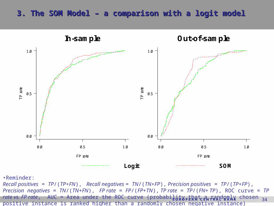
3. The SOM Model – a comparison with a logit model3. The SOM Model – a comparison with a logit model
•Reminder:Recall positives = TP/(TP+FN), Recall negatives = TN/(TN+FP), Precision positives = TP/(TP+FP), Precision negatives = TN/(TN+FN), FP rate = FP/(FP+TN), TP rate = TP/(FN+ TP), ROC curve = TP rate vs. FP rate, AUC = Area under the ROC curve (probability that a randomly chosen positive instance is ranked higher than a randomly chosen negative instance)
0.0 0.5 1.0
0.0
0.5
1.0
In-sample
FP rate
TP
ra
te
Logit SOM
0.0 0.5 1.0
0.0
0.5
1.0
Out-of-sample
FP rate
TP
ra
te
35
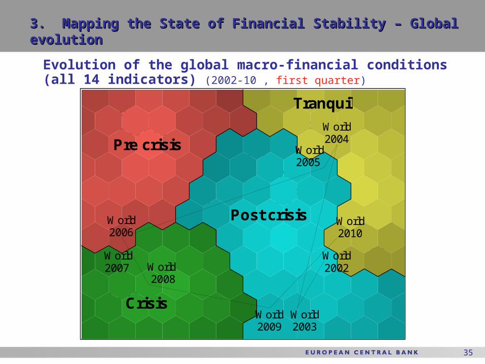
3. Mapping the State of Financial Stability – Global 3. Mapping the State of Financial Stability – Global evolutionevolution
Evolution of the global macro-financial conditions (all 14 indicators) (2002-10 , first quarter)
Pre-crisis
Crisis
Post-crisis
Tranquil
Crisis
Tranquil
Pre crisis
Post crisis
World 2004
World 2005
World 2006
World
2007 World 2002 World
2008
World 2009
World 2003
World 2010

36
4. Visual Analysis of Systemic Events 4. Visual Analysis of Systemic Events –– financial stability financial stability cyclecycle
Evolution of the macro-financial conditions in China (2007Q4-2010Q3, quarterly observations)
Pre-crisis
Crisis
Post-crisis
Tranquil
Crisis
Tranquil
Pre crisis
Post crisis
China 2010Q1
China 2009Q4
China 2008Q1
China
2008Q2
China 2009Q2
China2009Q1
China2008Q3-4
China 2009Q3 China
2010Q2-3
China 2007Q4

37
4. Visual Analysis of Systemic Events 4. Visual Analysis of Systemic Events –– financial stability financial stability cyclecycle
Evolution of the macro-financial conditions in Russia (2007Q4-2010Q3, quarterly observations)
Pre-crisis
Crisis
Post-crisis
Tranquil
Tranquil
Pre crisis
Post crisisRussia2007Q2-3
Russia 2010Q1-2
Russia
2007Q4 2008Q1-2
Russia2008Q4
2009Q1-2
Russia2009Q3
Russia 2009Q4
Russia2010Q3
Russia2008Q3
Crisis

38
Deleted slidesDeleted slides

39
1. Introduction - motivation1. Introduction - motivation
• Frequent occurrence of financial distressFrequent occurrence of financial distress• EWS literature based on conventional statistical EWS literature based on conventional statistical
techniques:techniques:– UnivariateUnivariate - signalling approach (e.g. KLR, 1997) - signalling approach (e.g. KLR, 1997)– MultivariateMultivariate - logit/probit models (e.g. Berg & - logit/probit models (e.g. Berg &
Pattillo, 1998)Pattillo, 1998)
• The above methods have certain The above methods have certain limitationslimitations::– No interactions No interactions between indicatorsbetween indicators– DistributionalDistributional assumptions on crisis probabilities assumptions on crisis probabilities– No visualizationNo visualization of multivariate data of multivariate data
• Non-parametricNon-parametric methods (Peltonen, 2006) methods (Peltonen, 2006)– Improve accuracy and predictive power, but do not Improve accuracy and predictive power, but do not
focus on visualizationfocus on visualization

40
1. Introduction - motivation1. Introduction - motivation
• Visualizing the state of financial stability is a Visualizing the state of financial stability is a
challenging task:challenging task:– Dimensionality problem: Dimensionality problem: as a large number of as a large number of
indicators are required to describe various aspects indicators are required to describe various aspects of vulnerabilities and to assess systemic risksof vulnerabilities and to assess systemic risks
– How to visualize multidimensional indicators How to visualize multidimensional indicators on on a static two/three dimensional chart?a static two/three dimensional chart?
– Temporal and cross-section Temporal and cross-section aspects complicates aspects complicates the matterthe matter
• Combining a method with a good visualization Combining a method with a good visualization capacitiy with a good capacitiy with a good out-of-sample predictionsout-of-sample predictions of of systemic events is even more challenging…systemic events is even more challenging…


