1 M a x e n t M o d e l s , C o n d i t i o n a l E s t i m a t i o n , a n d O p t i m i z a t i o n Dan Klein and Chris Manning S t anf o rd U niv ersit y ht t p : //nlp .st anf o rd.edu / HLT-N A A C L 2003 and A C L 2 0 0 3 Tu t o r i a l Without M a g ic That is, W ith M ath! I n t r o d u c t i o n In recent years there has been extensive use o f conditional o r dis cr im inativ e p ro babil istic m o d el s in N L P , IR , and S p eech B ecause: They give high accuracy performance They mak e it eas y t o incorporat e l ot s of l inguis t ical l y import ant feat ures They al l ow aut omat ic b uil d ing of l anguage ind epend ent , ret arget ab l e N L P mod ul es Joint vs. Conditional Models Joint (generative) models p lac e p rob ab ilities over b oth ob served data and th e h idden stu f f (gene- rate th e ob served data f rom h idden stu f f ): A ll th e b est k now n S tatN L P models: n-gram models, Naive Bayes classifiers, hidden M ark ov models, p rob ab ilist ic cont ex t -free grammars Discriminative (conditional) models tak e th e data as g iven, and p u t a p rob ab ility over h idden stru ctu re g iven th e data: L ogist ic regression, condit ional loglinear models, max imu m ent rop y mark ov models, ( S V M s, p ercep t rons) P (c, d) P (c| d) Bayes Net/Graphical Models B ay es net diag rams draw circles f or random variab les, and lines f or direct dep endencies S ome variab les are ob served; some are h idden E ach node is a little classif ier (conditional p rob ab ility tab le) b ased on incoming arcs c 1 c 2 c 3 d 1 d 2 d 3 HMM c d 1 d 2 d 3 N a i v e B a y e s c d 1 d 2 d 3 Generative L o g i s t i c R e g r e s s i o n D is c rim inative Conditional models work well: W ord S ense D isamb ig u ation Even with exactly the s am e f eatu r es , c ha ng ing f r o m j o int to c o nd itio na l es tim a tio n inc r ea s es p erform a nc e T ha t is , we u s e the s am e s m o o thing , a nd the s am e w o r d -clas s f ea tu r es , we j u s t c ha ng e the nu m bers ( p a r a m eter s ) T r a ining S et 9 8 . 5 C o nd . L ik e. 8 6 . 8 J o int L ik e. A c c u r a c y O b j ec tive T es t S et 7 6 . 1 C o nd . L ik e. 7 3 . 6 J o int L ik e. A c c u r a c y O b j ec tive (Klein and Manning 2002, using S ensev al-1 D at a) Overview: HLT Systems Typical Speech/NLP problems involve complex st ru ct u res ( seq u ences, pipelines, t rees, f eat u re st ru ct u res, sig nals) M od els are d ecomposed int o ind ivid u al local d ecision mak ing locat ions C ombining t hem t og et her is t he g lobal inf erence problem Sequence D a t a Sequence M o d el C o m b i ne l i t t l e m odels together via in f eren ce
Transcript
1
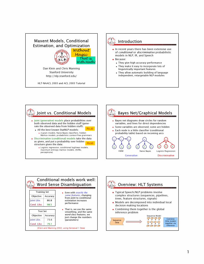
M a x e n t M o d e l s , C o n d i t i o n a l E s t i m a t i o n , a n d O p t i m i z a t i o n
Dan Klein and Chris ManningS t anf o rd U niv ersit y
ht t p : //nlp .st anf o rd.edu /
HLT-N A A C L 2 0 0 3 a n d A C L 2 0 0 3 Tu t o r i a l
WithoutM a g icThat is,
W ith M ath!
I n t r o d u c t i o n� In recent years there has been extensive use o f conditional o r dis cr im inativ e p ro babil istic m o d el s in N L P , IR , and S p eech
� B ecause:� They give high accuracy performance� They mak e it eas y t o incorporat e l ot s of l inguis t ical l y import ant feat ures
� They al l ow aut omat ic b uil d ing of l anguage ind epend ent , ret arget ab l e N L P mod ul es
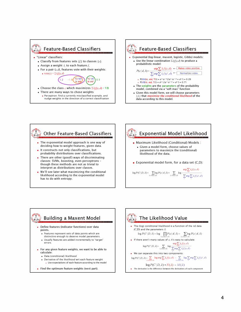
Joint vs. Conditional Models� Joint (generative) models p lac e p rob ab ilities over b oth ob served data and th e h idden stu f f (gene-rate th e ob served data f rom h idden stu f f ): � A ll th e b est k now n S tatN L P models:
� n-gram models, Naive Bayes classifiers, hidden M ark ov models, p rob ab ilist ic cont ex t -free grammars
� Discriminative (conditional) models tak e th e data as g iven, and p u t a p rob ab ility over h idden stru ctu re g iven th e data:
� L ogist ic regression, condit ional loglinear models, max imu m ent rop y mark ov models, ( S V M s, p ercep t rons)
P (c, d)
P (c| d)
Bayes Net/Graphical Models� B ay es net diag rams draw circles f or random variab les, and lines f or direct dep endencies
� S ome variab les are ob served; some are h idden� E ach node is a little classif ier (conditional p rob ab ility tab le) b ased on incoming arcs
c1 c2 c3
d1 d2 d3HMM
c
d1 d 2 d 3
N a i v e B a y e s
c
d1 d2 d3
Generative
L o g i s t i c R e g r e s s i o nD is c rim inative
Conditional models work well: W ord S ense D isamb ig u ation
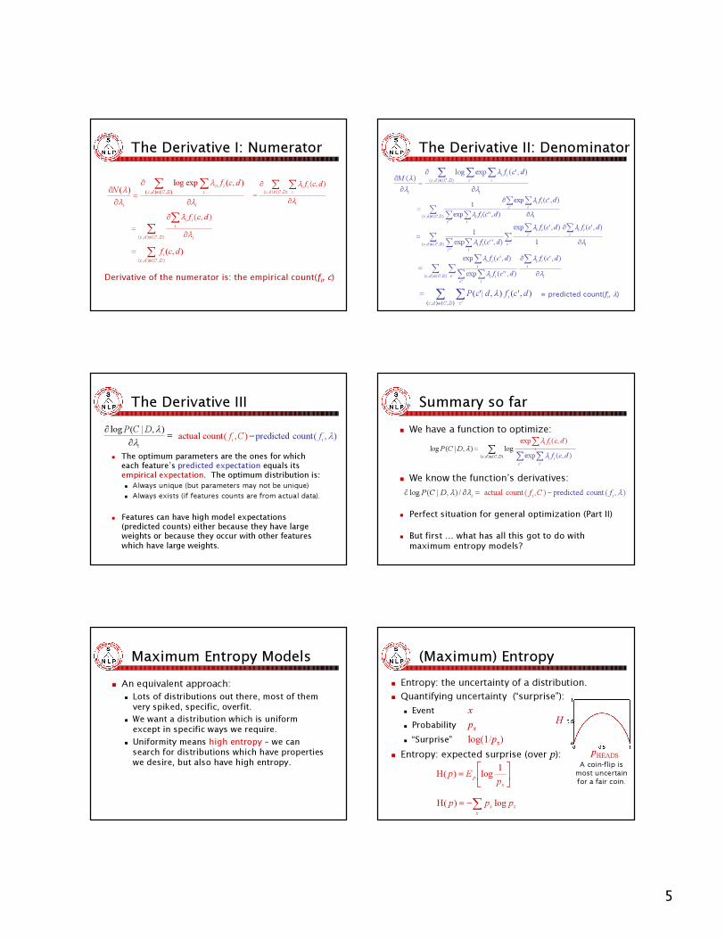
� Even with exactly the s am e f eatu r es , c ha ng ing f r o m j o int to c o nd itio na l es tim a tio n inc r ea s es p er f o r m a nc e
� T ha t is , we u s e the s a m e s m o o thing , a nd the s a m e w o r d -clas s f ea tu r es , we j u s t c ha ng e the nu m b er s ( p a r a m eter s )
T r a ining S et
9 8 . 5C o nd . L ik e.8 6 . 8J o int L ik e.
A c c u r a c yO b j ec tive
T es t S et
7 6 . 1C o nd . L ik e.7 3 . 6J o int L ik e.
A c c u r a c yO b j ec tive
(Klein and Manning 2002, using S ensev al-1 D at a)
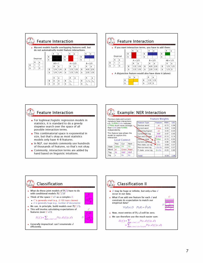
Overview: HLT Systems� Typical Speech/NLP problems involve complex st ru ct u res ( seq u ences, pipelines, t rees, f eat u re st ru ct u res, sig nals)
� M od els are d ecomposed int o ind ivid u al local d ecision mak ing locat ions
� C ombining t hem t og et her is t he g lobal inf erence problem
SequenceD a t a
Sequence M o d elC o m b i ne
l i t t l e m o d el stogether viain f eren c e
2
O v e r v i e w : T h e L o c a l L e v e lSequence Level
Lo ca l Level
LocalD at a
F e at u r eE x t r act i on
Features
L ab elO p t i m i z at i onS m oot h i n g
C las s i f i e r T y p e
Features
L ab el
S e q u e n ceD at a
M ax i m u m E n t r op y M od e ls
Q u ad r at i cP e n alt i e s
C on j u g at eG r ad i e n t
S e q u e n ce M od e l
N LP I s s u e s
I n f e r e n ce
LocalD at aLocalD at a
T u t o r i a l P l a n
1. Exponential/Maximum entropy models
2 . O ptimiz ation meth ods
3 . L ing uistic issues in using th ese models
Part I: Maximum Entropy Modelsa . Examples of F eature-B ased Modeling
b . Exponential Models f or C lassif ic ation
c . Maximum Entropy Models
d . S mooth ingWe will use the term “ma x en t” mo d els, b ut will
in tro d uc e them a s lo g lin ea r o r ex p o n en tia l mo d els, d ef errin g the in terp reta tio n a s “ma x imum en tro p y
mo d els” un til la ter.
Features� In this tutorial and most max e nt w ork :
features are e le me ntary p ie c e s of e v ide nc e that link asp e c ts of w hat w e ob se rv e d w ith a c ate g ory c that w e w ant to p re dic t.
� A f e ature has a re al v alue : f: C × D → R � U sually f e ature s are indic ator f unc tions of p rop e rtie s of the inp ut and a p artic ular c lass (ev ery o n e w e p resen t i s) . T he y p ic k out a sub se t.� fi(c, d ) ≡ [ Φ (d ) ∧ c = ci] [Value is 0 or 1]
� We will freely say that Φ(d) is a featu re o f the d ata d , when , fo r eac h ci , the c o n j u n c tio n Φ(d) ∧ c = ci is a featu re o f the d ata-c lass p air (c, d).
Features� For example:
� f1(c, d ) ≡ [c= “NN” ∧ i s l o w e r (w0) ∧ e n d s (w0, “d ”)]� f2( c , d ) ≡ [ c = “NN” ∧ w-1 = “t o ” ∧ t-1 = “T O ”]� f3( c , d ) ≡ [ c = “V B ” ∧ i s l o w e r (w0)]
� Models will assign each feature a weight� E m p irical count ( ex p ectation) of a feature:
� Model ex p ectation of a feature:
TO N Nto aid
I N J J in b l u e
TO V Bto aid
I N N Nin b e d
∑ ∈= ),(observed),( ),()( empirical
DCdc ii dcffE
∑ ∈= ),(),( ),(),()(
DCdc ii dcfdcPfE
Feature-B as ed M o d el s� The decision about a data point is based
onl y on the f eatur es activ e at that point.
BUSINESS: St o c k s h i t a y e a r l y l o w …
D a t a
F e a t u r e s{ … , s t o c k s , h i t , a , y e a r l y , l o w , … }
L a b e lBUSINESS
T e x t C a t e g o r i z a t i o n
… t o r e s t r u c t u r e b a n k :M O NEY d e b t .
D a t a
F e a t u r e s{ … , P = r e s t r u c t u r e , N= d e b t , L = 1 2 , … }
L a b e lM O NEY
W o r d -Se n s e D i s a m b i g u a t i o n
D T J J NN …T h e p r e v i o u s f a l l …
D a t a
F e a t u r e s{ W = f a l l , P T = J J P W = p r e v i o u s }
L a b e lNN
P O S T a g g i n g
3
E x a m p l e : T e x t C a t e g o r i z a t i o n(Zhang and O l e s 2 0 0 1 )� Features are a w o rd i n d o c um en t an d c l ass ( th ey d o f eature sel ec ti o n to use rel i ab l e i n d i c ato rs)
� T ests o n c l assi c R euters d ata set ( an d o th ers)� N aï v e B ay es: 7 7 . 0 % F1� Linear regression: 86.0%� Logist ic regression: 86.4 %� S u p p ort v ec t or m ac h ine: 86.5 %
� E m p h asiz es t h e im p ort anc e of regularization( sm oot h ing) f or su c c essf u l u se of d isc rim inat iv e m et h od s ( not u sed in m ost earl y N LP / I R w ork )
Example: NER(Klein et al. 2003; also, B or th w ic k 1 9 9 9 , etc .)� Sequence model across words� E ach word classi f i ed b y local model� F eat ures i nclude t h e word, p rev i ous
and nex t words, p rev i ous classes, p rev i ous, nex t , and current P O S t ag , ch aract er n- g ram f eat ures and s h a p e of word� Best model had > 800K features
� High (> 92% on English d e v t e st se t ) p e r f or m a nc e c om e s f r om c om b ining m a ny inf or m a t iv e f e a t u r e s.
� W it h sm oot hing / r e gu la r iz a t ion, m or e f e a t u r e s ne v e r hu r t ! X xX xxS i g
N N PN N PI NT agR oadG rac eatW ord? ? ?? ? ?O therC lassN extC urP rev
Local Context
D ec i si on P oi n t:S tate for Grace
Example: NER
0.370.6 8O-X xP r e v s t a t e , c u r s i g0.37-0.6 9x-X x-X xP r e v -c u r -n e xt s i g
2.68-0 .5 8T o t a l :…
0.8 2-0.2 0O-x-X xP . s t a t e - p-c u r s i g
0. 4 60. 8 0X xC u r r e n t s i g n a t u r e-0.9 2-0.70Ot h e rP r e v i o u s s t a t e0. 1 4-0.1 0I N N N PP r e v a n d c u r t a g s0. 4 50. 4 7N N PC u r r e n t P OS t a g-0.040.4 5<GB e g i n n i n g b i g r a m0.000.03Gr a c eC u r r e n t w o r d0. 9 4-0.73a tP r e v i o u s w o r dL O CP E R SF e a t u r eF e a t u r e T y p e
XxXxxS i gN N PN N PINT a gR o a dG r a c ea tW o r d? ? ?? ? ?O t h e rC l a s sNe x tC u rP r e v
Local Context
F eatu r e W ei g h ts( K l e i n e t a l . 2 0 0 3 )
D e c i s i o n P o i n t :S t a t e f o r Grace
Example: Tagging� Features can include:
� Current, previous, next words in isolation or together.� P revious ( or next) one, two, three tags.� W ord-internal f eatures: word ty pes, suf f ixes, dashes, etc .
%22. 6f e l lD o wT h e? ? ?? ? ?V B DN N PD T+ 10-1-2-3
Local ContextF eatu r es
trueh a s D i g i t?……
N N P -V B DT-1-T-2
V B DT-1f el lW-1
%W + 1
2 2 . 6W0
Decision Point
(R a t n a p a r k h i 1 9 9 6 ; T o u t a n o v a e t a l . 2 0 0 3 , e t c . )
Other M a x en t E x a m p l es� Sentence boundary detection (M i k h e e v 2 0 0 0 )
� Is period end of sentence or abbreviation?� P P attach m ent (R a t n a p a r k h i 1 9 9 8 )
� F eatu res of h ead nou n, preposition, etc.� L ang uag e m odel s (R o s e n f e l d 1 9 9 6 )
� P ( w 0|w-n , … , w-1 ) . F e a t u r e s a r e wo r d n -g r a m f e a t u r e s , a n d t r i g g e r f e a t u r e s wh i c h m o d e l r e p e t i t i o n s o f t h e s a m e wo r d .
� Parsing (R a t n a p a r k h i 1 9 9 7 ; J o h n s o n e t a l . 1 9 9 9 , e t c . )� E i t h e r : L o c a l c l a s s i f i c a t i o n s d e c i d e p a r s e r a c t i o n s o r f e a t u r e c o u n t s c h o o s e a p a r s e .
Conditional vs. Joint Likelihood� We have some data {(d, c)} an d w e w an t to p l ac e p r ob ab i l i ty di str i b u ti on s over i t.
� A joint model g i ves p r ob ab i l i ti es P (d, c) an d tr i es to max i mi z e thi s l i k el i hood.� It turns out to be trivial to choose weights: j ust relative f req uencies.
� A conditional m od el gives p robabilities P(c|d) . It tak es the d ata as given and m od els only the cond itional p robability of the class.� W e seek to m ax im iz e cond itional lik elihood .� H ard er to d o ( as we’ ll see… )� M ore closely related to classif ication error.
4
F e a t u r e -B a s e d C l a s s i f i e r s� “Linear” classifiers:
� C lassify fro m feat u res set s {fi} t o classes {c}.� A ssig n a w eig h t λi to each feature fi.� F or a p ai r ( c , d ) , features v ote w i th thei r w ei g hts :
� vote(c) = Σλifi( c , d )
� Choose the class c w hi ch m ax i m i z es Σλifi( c , d ) = V B� There are many ways to chose weights
� Perceptron: f i nd a cu rrentl y m i s cl a s s i f i ed ex a m pl e, a nd nu d g e w ei g h ts i n th e d i recti on of a correct cl a s s i f i ca ti on
TO N Nto aid
TO V Bto aid1 . 2 –1 . 8 0 . 3
Feature-B as ed C l as s i f i ers� Exponential (log-linear, m ax ent , lo g is t ic , G ib b s ) m o d els :
� U s e t h e linear c o m b inat io n Σλifi( c , d ) t o p ro d u c e a p ro b ab ilis t ic m o d el:
� P(N N |to, aid, T O ) = e1.2e–1.8 / (e1.2e–1. 8 + e 0 .3 ) = 0 . 2 9� P(V B |to, aid, T O ) = e 0 .3 / (e1.2e–1.8 + e 0 . 3 ) = 0 . 7 1
� The w ei g ht s a r e t he p a r a m et er s of the probability m od el, c om bin ed v ia a “s oft m ax ” fu n c tion
� G iv en this m od el form , w e w ill c hoos e param eters {λi} that maximize the conditional likelihood of the d ata ac c ord in g to this m od el.
∑ ∑'
),'(expc i
ii dcfλ=),|( λdcP ∑
iii dcf ),(exp λ Makes votes positive.
N or m al iz es votes.
Other Feature-B as ed C l as s i f i ers� The exponential model approach is one way of deciding how to weig ht featu res, g iv en data.
� I t constru cts not only classifications, b u t prob ab ility distrib u tions ov er classifications.
� There are other ( g ood! ) ways of discriminating classes: S V M s, b oosting , ev en perceptrons –thou g h these methods are not as triv ial to interpret as distrib u tions ov er classes.
� W e’ ll see later what maximiz ing the conditional lik elihood according to the exponential model has to do with entropy.
Exponential Model Likelihood� Maximum Likelihood (Conditional) Models :
� Given a model form, choose values of p aramet ers t o max imiz e t he ( condit ional) lik elihood of t he dat a.
� E xp onential model f or m, f or a data set (C, D ):
∑∑∈∈
==),(),(),(),(log),|(log),|(log
DCdcDCdcdcPDCP λλ
∑ ∑'
),'(expc i
ii dcfλ
∑i
ii dcf ),(exp λ
Building a M ax e nt M o de l� Define features (indicator functions) over data
p oints.� Features represent sets of data points which are
distinctiv e enoug h to deserv e m odel param eters.� U sual l y features are added increm ental l y to “ targ et”
errors.
� F or any g iven feature w eig h ts, w e w ant to b e ab l e to cal cul ate:� Data (conditional) likelihood� Der iv ativ e of the likelihood w r t each f eatu r e w eig ht
� Use expectations of each feature according to the model
� Find the optimum feature weights (next part).
The Likelihood Value� The (log) conditional likelihood is a function of the iid data
(C,D) and the p ar am eter s λ:
� I f ther e ar en’ t m any v alues of c, it’ s easy to calculate:
� W e can sep ar ate this into tw o com p onents:
� The derivative is the difference between the derivatives of each com p onent
∑∏∈∈
==),(),(),(),(
),|(log),|(log),|(logDCdcDCdc
dcPdcPDCP λλλ
∑∈
=),(),(log),|(log
DCdcDCP λ ∑ ∑
'
),(expc i
ii dcfλ∑i
ii dcf ),(exp λ
∑ ∑ ∑∈ ),(),( '
),'(explogDCdc c i
ii dcfλ∑ ∑∈ ),(),(
),(explogDCdc i
ii dcfλ −=),|(log λDCP
)(λN )(λM=),|(log λDCP −
5
T h e D e r i v a t i v e I : N u m e r a t o r
i
DCdc iii dcf
λ
λ
∂
∂=
∑ ∑∈ ),(),(
),(
∑∑
∈ ∂
∂=
),(),(
),(
DCdc i
iii dcfλ
λ
∑∈
=),(),(
),(DCdci dcf
i
DCdc iici
i
dcfNλ
λ
λλ
∂
∂=
∂∂ ∑ ∑
∈ ),(),(),(explog)(
Derivative of the numerator is: the empirical count(fi , c )
The Derivative II: Denominator
i
DCdc c iii
i
dcfMλ
λ
λλ
∂
∂=
∂∂ ∑ ∑ ∑
∈ ),(),( '),'(explog)(
∑∑ ∑
∑ ∑∈ ∂
∂=
),(),('
''
),'(exp),''(exp
1DCdc i
c iii
c iii
dcfdcf λ
λ
λ
∑ ∑∑∑
∑ ∑∈ ∂
∂=
),(),( '''
),'(1
),'(exp),''(exp
1DCdc c i
iii
iii
c iii
dcfdcfdcf λ
λλ
λ
i
iii
DCdc cc i
ii
iii dcf
dcfdcf
λ
λ
λ
λ
∂
∂=
∑∑ ∑∑ ∑
∑∈
),'(),''(exp
),'(exp
),(),( '''
∑ ∑∈
=
),(),( '),'(),|'(
DCdci
cdcfdcP λ = predicted count(fi , λ)
The Derivative III
� The optimum parameters are the ones for which each feature’ s pred icted ex pectation equals its em p ir ic al ex p ec tatio n . T h e o p tim um d istr ib utio n is:� Always unique (but parameters may not be unique)� Always ex ists (if f eatures c ounts are f rom ac tual d ata).
� F eatur es c an h av e h ig h m o d el ex p ec tatio n s ( p r ed ic ted c o un ts) eith er b ec ause th ey h av e lar g e w eig h ts o r b ec ause th ey o c c ur w ith o th er f eatur es w h ic h h av e lar g e w eig h ts.
� Lots of distributions out there, most of them v ery sp ik ed, sp ec ific , ov erfit.
� W e w a nt a distribution w hic h is uniform ex c ep t in sp ec ific w a y s w e req uire.
� U niformity mea ns hig h entrop y – w e c a n sea rc h for distributions w hic h ha v e p rop erties w e desire, but a l so ha v e hig h entrop y .
(Maximum) Entropy� Entropy: the uncertainty of a distribution.� Q uantifying uncertainty ( “ surprise” ) :
� E v ent x� Probability px� “ S u rp ris e ” log(1/px)
� Entropy: expected surprise (over p):
∑−=x
xx ppp log)(H
=x
p pEp 1log)(HA coin-f l ip is
m os t u nce r t a in f or a f a ir coin.
pHEADS
H
6
M a x e n t E x a m p l e s I� What do we want from a distribution?
� Minimize commitment = maximize entropy.� R es emb l e s ome ref erence d is trib u tion ( d ata) .
� S ol ution: max imiz e entrop y H , subj ec t to feature-based c onstraints:
� Adding constraints (features):� Lowers maximum entropy� R aises maximum l ik el ih ood of d ata� B ring s th e d istrib ution f urth er f rom unif orm� B ring s th e d istrib ution c l oser to d ata
[ ] [ ]ipip fEfE ˆ= ∑∈
=
ifxix Cp
Unconstrained, m ax at 0 . 5
C onstraint th at pHEADS = 0.3
Maxent E xam p l es I IH ( pH pT, ) pH + pT= 1 pH = 0.3
- x l o g x1/e
Maxent E xam p l es I I I� Lets say we have the following event space:
� … and the following em pir ical d ata:
� M ax im iz e H :
� … want pr ob ab ilities: E [ N N , N N S , N N P , N N P S , V B Z , V B D ] = 1
V B DV B ZN N P SN N PN N SN N
1/e1/e1/e1/e1/e1/e
1/61/61/61/61/61/6
13131153
Maxent E xam p l es I V� Too uniform!� N * a re more c ommon t h a n V * , s o w e a d d t h e fe a t ure fN = { N N ,
N N S , N N P , N N P S } , w i t h E [ fN ] = 3 2 / 3 6
� … a nd p rop e r nouns a re more fre q ue nt t h a n c ommon nouns , s o w e a d d fP = { N N P , N N P S } , w it h E [ fP ] = 2 4 / 3 6
� … w e c oul d k e e p re fining t h e mod e l s , e . g . b y a d d ing a fe a t ure t o d is t ing uis h s ing ul a r v s . p l ura l nouns , or v e rb t y p e s .
2/362/368 /368 /368 /368 /36
2/362/361 2/361 2/364 /364 /36
V B DV B ZN N P SN N PN N SN N
Feature Overlap� Maxent m o d el s h and l e o v er l ap p i ng f eatu r es w el l .� U nl i k e a N B m o d el , th er e i s no d o u b l e c o u nti ng !
12b12BaA
1/ 41/ 4b1/ 41/ 4BaA
E m p i r i c al
Al l = 1bB
aA
1/ 61/ 3b1/ 61/ 3BaA
A = 2/ 3bB
aA
1/ 61/ 3b1/ 61/ 3BaA
A = 2/ 3bB
aA
bB
aA
λAbλAB
aA
λ’A+λ’’Abλ’A+λ’’AB
aA
Example: NER Overlap
0.370.6 8O-X xP r e v s t a t e , c u r s i g0.37-0.6 9x-X x-X xP r e v -c u r -n e xt s i g
2.68-0.58T o t a l :…
0 . 8 2-0 . 2 0O-x-X xP . s t a t e - p-c u r s i g
0 . 4 60 . 8 0X xC u r r e n t s i g n a t u r e-0 . 9 2-0 . 7 0Ot h e rP r e v i o u s s t a t e0 . 1 4-0 . 1 0I N N N PP r e v a n d c u r t a g s0 . 4 50 . 4 7N N PC u r r e n t P OS t a g-0 . 0 40 . 4 5<GB e g i n n i n g b i g r a m0 . 0 00 . 0 3Gr a c eC u r r e n t w o r d0 . 9 4-0 . 7 3a tP r e v i o u s w o r dL O CP E R SF e a t u r eF e a t u r e T y p e
XxXxxS i gN N PN N PI NT a gR o a dG r a c ea tW o r d? ? ?? ? ?O t h e rS t a t eN e xtC u rP r e v
Local Context
F eatu r e W ei g h tsGrace is correlated w ith P E R S O N , b u t does n ot add m u ch ev iden ce on top ofalready k n ow in g p ref ix f eatu res.
7
F e a t u r e I n t e r a c t i o n� Maxent m o d el s h and l e o v er l ap p i ng f eatu r es w el l , b u t
d o no t au to m ati c al l y m o d el f eatu r e i nter ac ti o ns .
01b11BaA
1/ 41/ 4b1/ 41/ 4BaA
E m p i r i c al
Al l = 1bB
aA
1/ 61/ 3b1/ 61/ 3BaA
A = 2 / 3bB
aA
1/ 92 / 9b2 / 94 / 9BaA
B = 2 / 3bB
aA
00b00BaA
λAbλAB
aA
λAbλBλA+λBBaA
Feature Interaction� If you want interaction terms, you have to add them:
� A disj unctive feature woul d al so have done it ( al one) :
01b11BaA
Empirical
1 / 61 / 3b1 / 61 / 3BaA
A = 2 / 3bB
aA
1 / 92 / 9b2 / 94 / 9BaA
B = 2 / 3bB
aA
01 / 3b1 / 31 / 3BaA
AB = 1 / 3bB
aA
bB
aA
01 / 3b1 / 31 / 3BaA
Feature Interaction� For l og l i n e a r/ l og i s t i c re g re s s i on m od e l s i n s t a t i s t i c s , i t i s s t a n d a rd t o d o a g re e d y s t e p w i s e s e a rc h ov e r t h e s p a c e of a l l p os s i b l e i n t e ra c t i on t e rm s .
� T h i s c om b i n a t ori a l s p a c e i s e x p on e n t i a l i n s i z e , b u t t h a t ’ s ok a y a s m os t s t a t i s t i c s m od e l s on l y h a v e 4 –8 f e a t u re s .
� I n N L P , ou r m od e l s c om m on l y u s e h u n d re d s of t h ou s a n d s of f e a t u re s , s o t h a t ’ s n ot ok a y .
� C om m on l y , i n t e ra c t i on t e rm s a re a d d e d b y h a n d b a s e d on l i n g u i s t i c i n t u i t i on s .
E x am p l e: N E R Interaction
0.370.6 8O-X xPrev s t a t e, c u r s i g0 . 3 7-0 . 6 9x-X x-X xPrev-c u r-n ext s i g
2.68-0 .5 8T o t a l :…
0 . 8 2-0 . 2 0O-x-X xP. s t a t e - p-c u r s i g
0 . 4 60 . 8 0X xC u rren t s i g n a t u re-0 . 9 2-0 . 7 0Ot h erPrevi o u s s t a t e0 . 1 4-0 . 1 0I N N N PPrev a n d c u r t a g s0 . 4 50 . 4 7N N PC u rren t POS t a g-0 . 0 40 . 4 5<GB eg i n n i n g b i g ra m0 . 0 00 . 0 3Gr a c eC u rren t w o rd0 . 9 4-0 . 7 3a tPrevi o u s w o rdL O CP E R SF e a t u r eF e a t u r e T y p e
XxXxxS i gN N PN N PI NT a gR o a dG r a c ea tW o r d? ? ?? ? ?O t h e rS t a t eN e xtC u rP r e v
Local Context
F eatu r e W ei g h tsPrevious-st a t e a n d c urren t -sig n a t ure h a ve in t era c t ion s, e. g . P= PE R S -C = X x in d ic a t es C = PE R S m uc h m ore st ron g l y t h a n C = X x a n d P= PE R Sin d ep en d en t l y .T h is f ea t ure t y p e a l l ow s t h e m od el t o c a p t ure t h is in t era c t ion .
Classification� What do these joint models of P(X) have to do
w i th c on di ti on al m odel s P(C|D)?� T hi n k of the s p ac e C×D as a c om p l ex X.
� C is generally small (e.g., 2-100 topic classes)� D is g en er ally h u g e ( e. g . , n u m b er of d ocu m en ts)
� We can, in principle, build models over P(C,D).� T h i s w i l l i n v o l v e c a l c u l a t i n g e x p e c t a t i o n s o f
f e a t u r e s ( o v e r C×D ) :
� G e n e r a l l y i m p r a c t i c a l : c a n ’ t e n u m e r a t e de f f i c i e n t l y .
X
C×D
D
C
∑ ∈= ),(),( ),(),()(
DCdc ii dcfdcPfE
Classification II� D may be huge or infinite, but only a few d
oc c ur in our d ata. � W hat if we ad d one feature for eac h d and
c ons train its ex p ec tation to matc h our emp iric al d ata?
� N ow, mos t entries of P( c , d ) will be z ero.� W e c an therefore us e the muc h eas ier s um:
)(ˆ)()( dPdPDd =∈∀
∑ ∈= ),(),( ),(),()(
DCdc ii dcfdcPfE∑ >∧∈
= 0)(ˆ),(),( ),(),(dPDCdc i dcfdcP
D
C
8
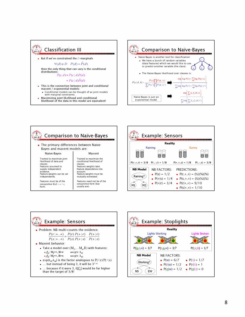
C l a s s i f i c a t i o n I I I� But if we’ve constrained the D m arg inal s
then the onl y thing that can vary is the conditional distrib utions:
� T his is the connection b etween j oint and conditional m ax ent / ex p onential m odel s:� Conditional models can be thought of as joint models
w ith mar ginal constr aints.� M ax im iz ing j oint l ik el ihood and conditional
l ik el ihood of the data in this m odel are eq uival ent!
)(ˆ)|()()|(),(
dPdcPdPdcPdcP
=
=
)(ˆ)()( dPdPDd =∈∀
Comparison to Naïve-B ay es� Naïve-B ay es i s an o t h er t o o l f o r c l as s i f i c at i o n :
� W e h ave a b u n c h o f r an d o m var i ab l es ( d at a f eat u r es ) w h i c h w e w o u l d l i k e t o u s e t o p r ed i c t an o t h er var i ab l e ( t h e c l as s ) :
� T h e Naïve-B ay es l i k el i h o o d o ver c l as s es i s :
c
φ1 φ 2 φ 3
=),|( λdcP ∏i
i cPcP )|()( φ∑ ∏
')'|()'(
c ii cPcP φ
+∑i
i cPcP )|(log)(logexp φ
∑ ∑
+'
)'|(log)'(logexpc i
i cPcP φ
∑i
icic cdf ),(exp λ
∑ ∑
'
'' )',(expc i
icic cdfλNaïve-B ay es i s j u s t an ex p o n en t i al m o d el .
Comparison to Naïve-B ay es� The primary differences between Naïve-
B ayes and max ent mo del s are:Naïve-B a y e s M a x e n t
Features assumed to sup p l y i n dep en den t ev i den c e.
Features w ei g h ts tak e f eature dep en den c e i n to ac c oun t.
Feature w ei g h ts c an b e set i n dep en den tl y .
Feature w ei g h ts must b e mutual l y esti mated.
Features must b e of th e c on j un c ti v e Φ(d) ∧ c = cif orm.
Features n eed n ot b e of th e c on j un c ti v e f orm ( b ut usual l y are) .
T rai n ed to max i mi z e j oi n t l i k el i h ood of data an d c l asses.
T rai n ed to max i mi z e th e c on di ti on al l i k el i h ood of c l asses.
Example: Sensors
NB FACTORS:� P ( s ) = 1 / 2 � P ( + | s ) = 1 / 4 � P ( + | r ) = 3 / 4
Raining S u nny
P(+,+,r) = 3/8 P(+,+,s ) = 1 /8
Reality
P(-,-,r) = 1 /8 P(-,-,s ) = 3/8
Raining?
M 1 M 2
NB Model PREDICTIONS:� P( r , + , + ) = ( ½ ) ( ¾ ) ( ¾ )� P( s , + , + ) = ( ½ ) ( ¼ ) ( ¼ )� P( r | + , + ) = 9 / 1 0� P( s | + , + ) = 1 / 1 0
Example: Sensors� Pr o b l e m : NB m u l t i -c o u n t s t h e e v i d e n c e .
� M a x e n t b e h a v i o r :� Take a model over (M1, … Mn, R ) w i t h f eat u res :
� fri: Mi= + , R = r weight: λri� fsi: Mi= + , R = s weight: λs i
� exp(λri-λs i) i s t h e f a c t o r a n a l o g o u s t o P(+|r)/P(+|s)� … b u t i n s t ea d o f b ei n g 3 , i t w i l l b e 3 1/n
� … because if it were 3, E[fri] wo ul d be far h ig h er th an th e targ et o f 3/ 8 !
)|()|(...)|(
)|()()(
)...|()...|(
sPrP
sPrP
sPrP
sPrP
+
+
+
+=
++
++
Example: StoplightsLights Working Lights B roke n
P ( g,r,w) = 3 / 7 P ( r,g,w) = 3 / 7 P ( r,r,b) = 1 / 7
� We’ ll gu ess that ( r, r) indic ates lights are work ing!
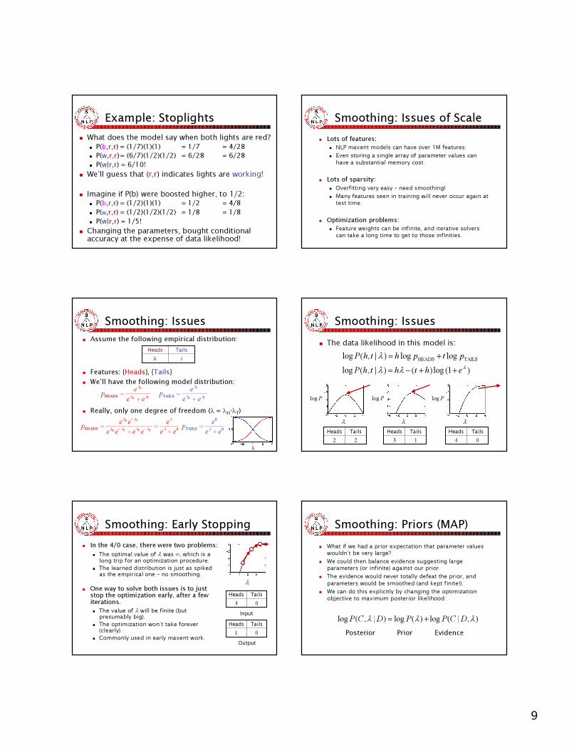
� I magine if P ( b) were boosted higher, to 1 / 2 :� P(b,r ,r ) = (1 / 2 )(1 )(1 ) = 1 / 2 = 4 / 8� P(w,r ,r ) = (1 / 2 )(1 / 2 )(1 / 2 ) = 1 / 8 = 1 / 8� P(w|r ,r ) = 1/5!
� Changing the parameters, bought conditional accuracy at the ex pense of data lik elihood!
Smoothing: Issues of Scale� Lots of features:
� NLP m a x e n t m o d e l s c a n h a v e o v e r 1 M f e a t u r e s .� E v e n s t o r i n g a s i n g l e a r r a y o f p a r a m e t e r v a l u e s c a n h a v e a s u b s t a n t i a l m e m o r y c o s t .
� Lots of sparsity:� O v e r f i t t i n g v e r y e a s y – n e e d s m o o t h i n g !� M a n y f e a t u r e s s e e n i n t r a i n i n g w i l l n e v e r o c c u r a g a i n a t t e s t t i m e .
� O ptim iz ation prob l e m s:� F e a t u r e w e i g h t s c a n b e i n f i n i t e , a n d i t e r a t i v e s o l v e r s c a n t a k e a l o n g t i m e t o g e t t o t h o s e i n f i n i t i e s .
Smoothing: Issues� Assume the following empirical distribution:
� F eatures: { H eads}, { T ails}� W e’ ll hav e the following model distribution:
� R eally , only one degree of freedom ( λ = λH-λT)
thTailsH e ad s
TH
H
HEADS λλ
λ
eeep+
=TH
T
TAILS λλ
λ
eeep+
=
0HEADS TTTH
TH
eee
eeeeeep
+=
+=
−−
−
λ
λ
λλλλ
λλ
0
0
TAILS eeep+
= λ
λ
Smoothing: Issues� The data likelihood in this model is:
Smoothing: Early Stopping� In the 4/0 case, there were two problems:
� The optimal value of λ w as ∞, w hic h is a lon g tr ip for an optimiz ation pr oc ed ur e.
� The lear n ed d is tr ib ution is j us t as s pik ed as the empir ic al on e – n o s moothin g .
� O ne way to solv e both i ssu es i s to j u st stop the opti mi z ati on early , af ter a f ew i terati ons.� The value of λ w ill b e fin ite ( b ut
pr es umab ly b ig ) .� The optimiz ation w on ’ t tak e for ever
( c lear ly ) .� C ommon ly us ed in ear ly max en t w or k .
04TailsH e ad s
01TailsH e ad s
I n p u t
O u t p u t
λ
Smoothing: Priors (MAP)� What if we had a prior expectation that parameter values
wouldn’ t b e very larg e?� We could then b alance evidence sug g esting larg e
parameters ( or infinite) ag ainst our prior.� T he evidence would never totally defeat the prior, and
parameters would b e smoothed ( and k ept finite! ) .� We can do this explicitly b y chang ing the optimiz ation
ob j ective to maximum posterior lik elihood:
),|(log)(log)|,(log λλλ DCPPDCP +=
Posterior Prior E v id en c e
10
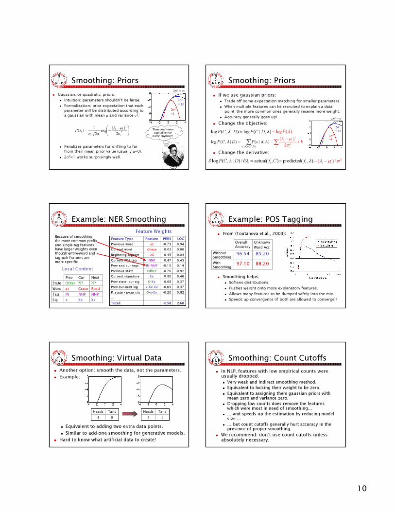
S m o o t h i n g : P r i o r s� Gaussian, o r q uad r at ic , p r io r s:
� I nt uit io n: p ar am e t e r s sh o ul d n’ t b e l ar g e .� F o r m al iz at io n: p r io r e x p e c t at io n t h at e ac h
p ar am e t e r w il l b e d ist r ib ut e d ac c o r d ing t o a g aussian w it h m e an µ and v ar ianc e σ2.
� P e nal iz e s p ar am e t e r s f o r d r if t ing t o f ar f r o m t h e ir m e an p r io r v al ue ( usual l y µ=0 ) .
� 2σ2=1 w o r k s sur p r ising l y w e l l .
They don’t even c a p i ta l i z e m y
na m e a nym or e!
−−= 2
2
2)(exp2
1)(i
ii
iiP σ
µλπσλ
2σ2
= 1
2σ2
= 1 0
2σ2 = ∞
Smoothing: Priors� If we use g a ussi a n p r i o r s:
� Trade off some expectation-match ing for smal l er parameters.� W h en mu l tipl e featu res can b e recru ited to expl ain a data
point, th e more common ones g eneral l y receiv e more w eig h t.� A ccu racy g eneral l y g oes u p!
� Change the objective:
� Change the d er ivative:
)(log λP−),|(log)|,(log λλ DCPDCP =
∑∈
=),(),(
),|()|,(logDCdc
dcPDCP λλ ki i
ii +−
−∑ 2
2
2)(
σµλ
),(predicted),(actual/)|,(log λλλ iii fCfDCP −=∂∂ 2/)( σµλ ii −−
2σ2
=1
2σ2
= 10
2σ2 = ∞
Example: NER Smoothing
0.370.6 8O-X xP r e v s t a t e , c u r s i g0.37-0.6 9x-X x-X xP r e v -c u r -n e xt s i g
2.68-0 .5 8T o t a l :…
0.8 2-0.2 0O-x-X xP . s t a t e - p-c u r s i g
0. 4 60. 8 0X xC u r r e n t s i g n a t u r e-0.9 2-0.70Ot h e rP r e v i o u s s t a t e0. 1 4-0.1 0IN NNPPr e v a n d c u r t a g s0 . 4 50 . 4 7NNPC u r r e n t PO S t a g-0 . 0 40 . 4 5<GB e g i n n i n g b i g r a m0 . 0 00 . 0 3Gr a c eC u r r e n t w o r d0 . 9 4-0 . 7 3a tPr e v i o u s w o r dLOCP E R SF e a t u r eF e a t u r e T y p e
XxXxxS i gN N PN N PI NT a gR o a dG r a c ea tW o r d? ? ?? ? ?O t h e rS t a t eN e xtC u rP r e v
Local Context
Feature WeightsBecause of smoothing, the mor e common p r efix and singl e-tag featur es hav e l ar ger w eights ev en though entir e-w or d and tag-p air featur es ar e mor e sp ecific.
Example: POS Tagging� From (Toutanova et al., 2003):
� S mooth i ng h elp s :� Softens distributions.� P ush es w eig h t onto m ore ex p l a na tory fea tures.� A l l ow s m a ny fea tures to be dum p ed sa fel y into th e m ix .� Sp eeds up c onv erg enc e ( if both a re a l l ow ed to c onv erg e) !
88.209 7 .1 0With S m o o thin g
85 .209 6 .5 4Witho u t S m o o thin g
U n k n o w n Wo r d A c c
O v e r a l l A c c u r a c y
Smoothing: Virtual Data� Another option: smooth the data, not the parameters.� E x ampl e:
� E q u iv al ent to adding tw o ex tra data points.� S imil ar to add-one smoothing f or g enerativ e model s.
� H ard to k now w hat artif ic ial data to c reate!
04TailsH e ad s
15TailsH e ad s
Smoothing: Count Cutoffs� I n N L P , f eatu res w ith l ow empiric al c ou nts w ere
u su al l y dropped.� Very weak and indirect smoothing method.� E q u iv al ent to l ocking their weight to b e z ero.� E q u iv al ent to assigning them gau ssian p riors with mean z ero and v ariance z ero.
� D rop p ing l ow cou nts does remov e the f eatu res which were most in need of smoothing…
� … and sp eeds u p the estimation b y redu cing model siz e …
� … b u t cou nt cu tof f s general l y hu rt accu racy in the p resence of p rop er smoothing.
� We recommend: don’t use count cutoffs unless a b solutely necessa ry .
11
P a r t I I : O p t i m i z a t i o n
a. Unconstrained optimization methods
b . C onstrained optimization methods
c . D u al ity of max imu m entropy and ex ponential model s
F u n c t i o n O p t i m i z a t i o n� To estimate the parameters of a maximum likelihood
model, w e must fin d the λ w hic h maximiz es:
� We’ll approach this as a general function optim iz ation prob lem , though special-purpose m ethod s ex ist.
� A n ad v antage of the general-purpose approach is that no m od ification need s to b e m ad e to the algorithm to support sm oothing b y priors.
∑ ∑ ∑∑
∈
=),(),(
'),'(exp
),(explog),|(log
DCdcc i
ii
iii
dcfdcf
DCPλ
λλ
Notation� Assume we have a
f un c t i o n f(x) from Rn t o R.
� T h e g ra d i e n t ∇f(x)i s t h e n×1 v e c t or of p a rt i a l d e ri v a t i v e s ∂f/∂xi.
� T h e H e s s i a n ∇2f i s t h e n×n m a t r i x o f s e c o n d d e r i v a t i v e s ∂2f/ ∂xi∂xj.
∂∂
∂∂=∇
nxf
xff
/
/ 1
M
∂∂∂∂∂∂
∂∂∂∂∂∂=∇
nnn
n
xxfxxf
xxfxxff
//
//
21
2
12
112
2
L
MOM
L
f
Taylor Approximations� Constant (z e r oth -or d e r ) :
� L i ne ar (f i r st-or d e r ) :
� Q u ad r ati c (se c ond -or d e r ) :
)()( 000
xfxf x =
)()( 010
xfxf x = )()( 0T
0 xxxf −∇+
))(()(21
002T
0 xxxfxx −∇−+
)()( 020
xfxf x = )()( 0T
0 xxxf −∇+
Unconstrained Optimization� Problem:
� Q u es t i on s :� Is there a unique maximum?� H o w d o w e f ind it ef f ic ientl y ?� D o es f hav e a sp ec ial f o rm?
� O u r s i t u a t i on :� f is convex.� f’ s f ir st d er iva t ive vect or ∇f is k now n.� f’ s second d er iva t ive m a t r ix ∇2f is not a va il a b l e.
)(maxarg* xfxx
=
Convexity)( ii
ixfw∑ 1=∑ i
iw)( ii
ixwf ∑ ≥
)(xfw∑
)( xwf ∑
Convex N on-ConvexConvexity guarantees a single, global maximum bec ause any h igh er p oints are greed ily reac h able.
12
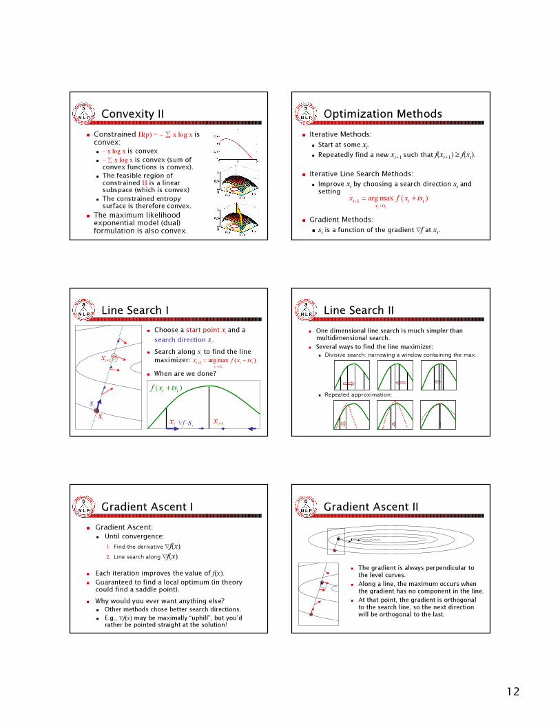
C o n v e x i t y I I� Constrained H(p) = – ∑ x l o g x is
c onv ex :� – x l o g x is convex� – ∑ x l o g x is convex ( su m of convex f u nct ions is convex) .
� T h e f ea sib l e r eg ion of const r a ined H is a l inea r su b sp a ce ( w h ich is convex)
� T h e const r a ined ent r op y su r f a ce is t h er ef or e convex.
� The maximum likelihood exp on en t ial model ( dual) f or mulat ion is als o c on v ex.
Optimization Methods� Iterative Methods:
� Start at some xi.� R ep eated l y f i n d a n ew xi+1 such that f(xi+1) ≥ f(xi ) .
� Iterative Line Search Methods:� Improve xi b y c h oos i n g a s ea rc h d i rec t i on si a n d s et t i n g
� G radient Methods:� si i s a f u n c t i on of t h e g ra d i en t ∇f at xi.
)(maxarg1 iitsx
i tsxfxii
+=+
+
Line Search I� Choose a st ar t p oi n t xi an d a search direction si.
� S earch al ong si to f ind the l ine m ax im iz er:
� W hen are w e done?
sixi
xi+1 )(maxarg1 iitsx
i tsxfxii
+=+
+
xi xi+1∇f ⋅si
)( ii tsxf +
Line Search II� One dimensional line search is much simpler than
multidimensional search.� S ev eral w ay s to f ind the line max imiz er:
� Divisive search: narrowing a window containing the max.
� R ep eated ap p roximation:
Gradient Ascent I� Gradient Ascent:
� Until convergence:1. Find the derivative ∇f(x).2 . L ine s earc h al o ng ∇f(x).
� E a ch itera tion im p roves th e va lu e of f(x).� Guaranteed to find a local optimum (in theory
could find a s addle point) .� W hy w ould you ev er w ant anything els e?
� Other methods chose better search directions.� E.g., ∇f(x) m a y b e m a x i m a l l y “ u p h i l l ” , b u t y o u ’ d
r a t h e r b e p o i n t e d s t r a i gh t a t t h e s o l u t i o n !
Gradient Ascent II
� T h e gr a d i e n t i s a l w a y s p e r p e n d i c u l a r t o t h e l e v e l c u r v e s .
� A l o n g a l i n e , t h e m a x i m u m o c c u r s w h e n t h e gr a d i e n t h a s n o c o m p o n e n t i n t h e l i n e .
� A t t h a t p o i n t , t h e gr a d i e n t i s o r t h o go n a l t o t h e s e a r c h l i n e , s o t h e n e x t d i r e c t i o n w i l l b e o r t h o go n a l t o t h e l a s t .
13
W h a t G o e s W r o n g ?� Graphically:
� Each new gradient is orthogonal to the previous line search, so we’ ll k eep m ak ing right-angle turns. I t’ s lik e b eing on a city street grid, try ing to go along a diagonal – y ou’ ll m ak e a lot of turns.
� M at he m at ically:� W e’ ve j ust searched along the old gradient direction si-1 = ∇f(xi-1) .� T h e n e w g r a d i e n t i s ∇f(xi) a n d w e k n o w si-1T⋅∇f(xi) = ∇f(xi-1)T⋅∇f(xi) = 0 .� A s w e m o v e a l o n g si = ∇f(xi), the gradient becomes ∇f(xi+tsi) ≈ ∇f(xi) + t∇2f(xi) si = ∇f(xi) + t∇2f(xi)∇f(xi).� What about that old direction si-1?
� si-1T ⋅ (∇f(xi-1) + t∇2f(xi)∇f(xi)) =
� ∇f(xi-1)T∇f(xi) + t∇f(xi-1)T∇2f(xi)∇f(xi) =� 0 + t∇f(xi-1)T∇2f(xi)∇f(xi)� … so the gradient is regrow ing a c om p onent in the l ast direc tion!
Conjugacy I� Problem: with gradient ascent,
search along si ru ined op timiz ation in p rev iou s directions.
� I dea: choose si to k eep the gradient in the p rev iou s direction( s) z ero.� I f we choose a direction si, we want:
� ∇f(xi+tsi) to stay orthogonal to previous s� si-1
� If ∇2f(x) i s c o n s t a n t , t h e n w e w a n t : si-1T∇2f(x)si = 0
Conjugacy I I� The condition si-1T∇2f(xi)si = 0a l m os t s a y s tha t the new
direction and the last should be orthog onal – it say s that they m ust be ∇2f(xi)-orthog onal, or conj ug ate.
� V arious w ay s to op erationaliz e this condition.
� B asic p roblem s:� We generally don’t know ∇2f(xi).� I t wou ldn’t f i t i n m em ory anyway.
si-1
si
∇f(xi)
Orthogonal C onj u gate
Conjugate Gradient Methods� The general CG method:
� U nti l c onv ergenc e:1. F i n d t h e d e r i v a t i v e ∇f(xi).2 . R e m o v e c o m p o n e n t s o f ∇f(xi) n o t c o n j u g a t e t o p r e v i o u s d i r e c t i o n s .3 . L i n e s e a r c h a l o n g t h e r e m a i n i n g , c o n j u g a t e p r o j e c t i o n o f ∇f(xi).
� The variations are in step 2.� If we know ∇2f(xi) a nd t r a c k a l l p r ev i ou s s ea r c h d i r ec t i ons , we c a n i m p l em ent t h i s d i r ec t l y .� If we d o not know ∇2f(xi) – we d on’ t for m a x ent m od el i ng – a nd i t
i s n’ t c ons t a nt ( i t ’ s not ) , t h er e a r e ot h er ( b et t er ) wa y s .� Sufficient to ensure conj ug a cy to th e sing l e p rev ious d irection.� C a n d o th is w ith th e fol l ow ing recurrences [ F l etch er-R eev es] :
1)(−
+∇= iiii sxfs β )()()()(11 −
Τ−
Τ
∇∇∇∇=
ii
iii xfxf
xfxfβ
Constrained Optimization� Goal:
s u b j e c t t o t h e c on s t r ai n t s :
� P r ob le m s :� Have to ensure we satisfy the constraints.� N o g uarantee that ∇f(x*) = 0 , so how to r e c og n i z e the m a x ?
� Solution: the method of Lagrange Multipliers
)(maxarg* xfxx
=
0)(: =∀ xgi i
Lagrange Multipliers I� At a g l o b al m ax , ∇f(x*) = 0.� Inside a constraint region,
∇f(x*) can b e non-z ero, b u tits p roj ection inside th econstraint m u st b e z ero.
� In tw o dim ensions, th is m eans th at th e gradientm u st b e a m u l tip l e of th e constraint norm al :
I l ov e th is p art.
= )(xg∇λ)(xf∇
14
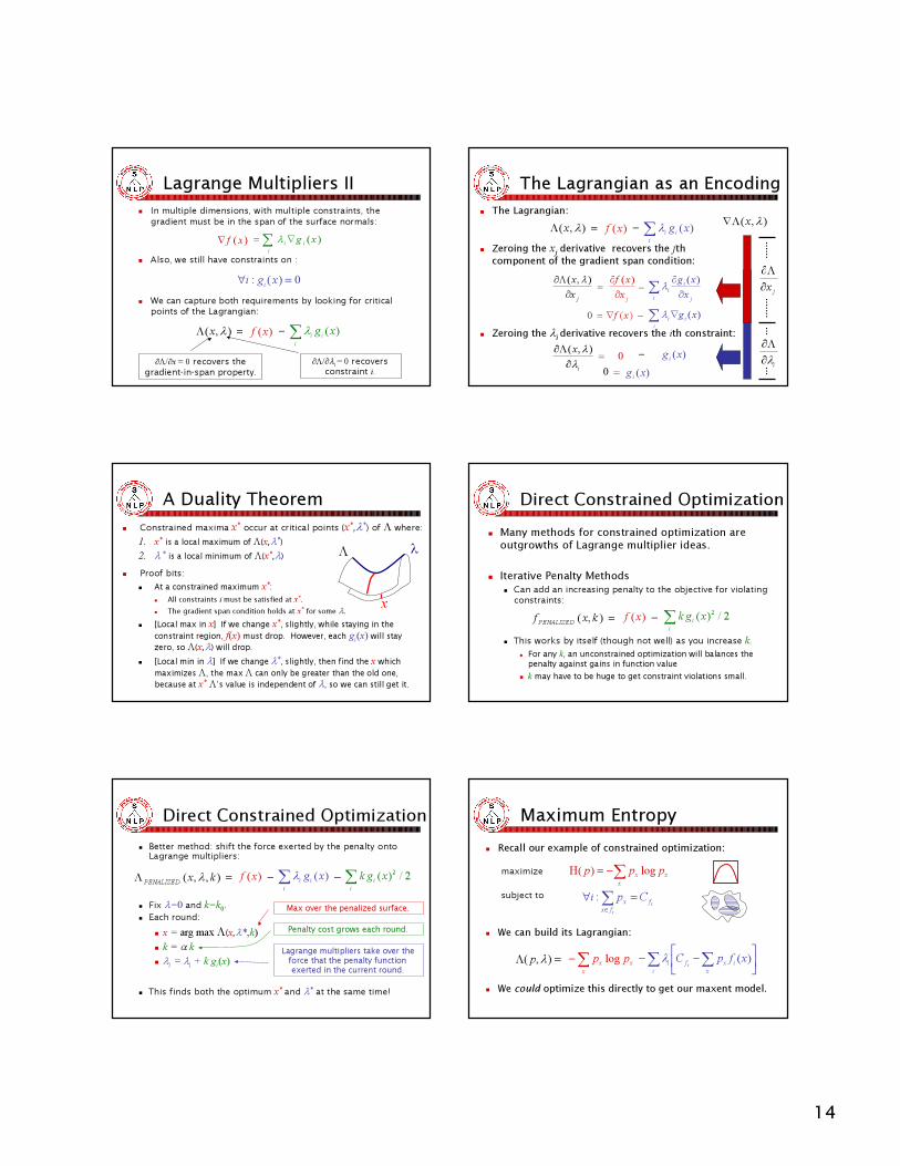
L a g r a n g e M u l t i p l i e r s I I� In multiple dimensions, with multiple constraints, the
g radient must b e in the span of the surf ace normals:
� A lso, we still hav e constraints on :
� W e can capture b oth req uirements b y look ing f or critical points of the L ag rang ian:
=∑ ∇i
ii xg )(λ)(xf∇
− ∑i
ii xg )(λ)(xf=Λ ),( λx
∂Λ/∂x = 0 recovers the g ra d i en t-i n -sp a n p rop erty .
∂Λ/∂λi = 0 recovers con stra i n t i.
0)(: =∀ xgi i
The L a g r a n g i a n a s a n E n c o d i n g� The Lagrangian:
� Z e ro ing t h e xj d e riv at iv e re c o v e rs t h e j t hc o m p o ne nt o f t h e grad ie nt s p an c o nd it io n:
� Z e ro ing t h e λi d e riv at iv e re c o v e rs t h e it h c o ns t raint :
− ∑i
ii xg )(λ)(xf=Λ ),( λx
− ∑ ∂∂
i j
ii x
xg )(λjxxf
∂∂ )(=
∂Λ∂
jx
x ),( λ
− )(xg i0=∂
Λ∂i
x
λλ ),(
− ∑ ∇i
ii xg )(λ)(xf∇=0
)(xg i=0
),( λxΛ∇
jx∂Λ∂
iλ∂Λ∂
A Duality Theorem� Constrained m ax im a x* oc c u r at c ritic al p oints ( x*,λ* ) of Λ w h ere:
1. x* is a local maximum of Λ(x,λ*)2 . λ * is a local min imum of Λ(x*,λ)
� Proof bits:� At a constrained maximum x*:
� All constraints i m u st b e satisf ie d at x*.� T h e g r a d i e n t s p a n c o n d i t i o n h o l d s a t x* f o r s o m e λ.
� [Local max in x] If we change x*, s l i ght l y , whi l e s t ay i ng i n t he co ns t r ai nt r egi o n, f(x) m u s t d r o p . H o wev er , each gi(x) wi l l s t ay z er o , s o Λ(x,λ ) wi l l d r o p .
� [ L o cal m i n i n λ] If we change λ*, s l i ght l y , t hen fi nd t he x whi ch m ax i m i z es Λ, t he m ax Λ can o nl y b e gr eat er t han t he o l d o ne, b ecau s e at x* Λ’ s v al u e i s i nd ep end ent o f λ , s o we can s t i l l get i t .
x
λΛ
Direct Constrained Optimization� Many methods for constrained optimization are
ou tg row ths of L ag rang e mu l tipl ier ideas.
� I terativ e P enal ty Methods� Can add an increasing penalty to the objective for violating
constraints:
� T his w ork s by itself ( thou gh not w ell) as you increase k.� For any k , an u nc ons t rai ne d op t i m i z at i on w i l l b al anc e s t h e
p e nal t y ag ai ns t g ai ns i n f u nc t i on v al u e� k may have to be huge to get constraint violations small.
− 2/)( 2∑i
i xgk)(xf=),( kxfPENALIZED
Direct Constrained Optimization� Better method: shift the force exerted by the penalty onto
L ag rang e mu ltipliers:
� F ix λ=0 and k =k 0.� E ach rou nd:
� x = arg m ax Λ(x,λ*,k)� k = α k� λi = λi + k gi(x)
� This finds both the optimum x* a nd λ* a t the sa me time!
− 2/)( 2∑i
i xgk)(xf=Λ ),,( kxPENALIZED λ ∑i
ii xg )(λ −
Max over the penalized surface.
Penalty cost grows each round.
L agrange m ulti p li ers tak e ov er the f orce that the p enalty f uncti on ex erted i n the current round.
Maximum Entropy� Recall our example of constrained optimization:
� W e can b uild its L ag rang ian:
� W e could optimize th is directly to g et our maxent model.
∑−=x
xx ppp log)(H
ii
ffx
x Cpi =∀ ∑∈
:
maximize
s u b j ec t t o
∑−x
xx pp log=Λ ),( λp ∑ ∑
−−i x
ixfi xfpCi
)(λ
15
L a g r a n g i a n : M a x -a n d -M i n� Can think of constrained optimization as:
� P enal ty methods w ork somew hat in this w ay :� Stay in the constrained region, or your function value
gets clob b ered b y p enalties.� Duality lets you reverse the ordering:
� Dual m ethods w ork in this w ay:� Solve the maximization for a given set of λs.� O f these solu tions, minimize over the sp ac e of λs.
− ∑i
ii xg )(λ)(xf=Λ ),( λxλ
minx
max
− ∑i
ii xg )(λ)(xf=Λ ),( λxλ
minx
max
The Dual Problem� For fixed λ , w e k n ow t h a t Λ h a s a m a xim u m w h ere:
� … a n d:
� … s o w e k n ow :
=∂
Λ∂xpp ),( λ
x
x
xx
p
pp
∂
∂− ∑ log
x
i xixii
pxfpC
∂
−∂−+
∑ ∑ )(λ0=
x
x
x
xx
pp
pplog1
log+=
∂
∂∑∑
∑ ∑−=∂
−∂i
iix
i xixii
xfpxfpC
)()(
λλ
)(log1 xfp ii
ix ∑=+ λ
)(exp xfp ii
ix ∑∝ λ
The Dual Problem� We know the maximum entropy distribution has the
exponential f orm:
� B y the dual ity theorem, we want to f ind the mul tipl iers λ that minimize the L ag rang ian:
� T he L ag rang ian is the neg ativ e data l og -l ikel ihood ( next sl ides) , so this is the same as f inding the λ whic h maximiz e the data l ikel ihood – our orig inal probl em in part I .
)(exp)( xfp ii
ix ∑∝ λλ
∑−x
xx pp log=Λ ),( λp ∑ ∑
−−i x
ixfi xfpCi
)(λ
The Dual Problem
∑−x
xx pp log=Λ ),( λp ∑ ∑
−−i x
ixfi xfpCi
)(λ
∑ ∑ ∑∑
−
xx i
ii
iii
x xfxf
p'
)'(exp)(exp
logλ
λ∑ ∑
−−
i xixfi xfpC
i)(λ
+
− ∑ ∑∑ ∑'
)'(explog)(x i
iix i
iix xfxfp λλ
+− ∑ ∑∑x i
iixfi
i xfpCi
)(λλ
=
=
The Dual Problem
∑ ∑x i
ii xf )(explog λif
iiC∑− λ=Λ ),( λp )(ˆ xfpC i
xxfi ∑=
∑ ∑x i
ii xf )(explog λ ∑∑−
xii
ix xfp )(ˆ λ
∑ ∑−
x iiix xfp )(explogˆ λ
∑ ∑
x iii xf )(explog λ
− ∑ ∑
∑∑
x iii
iii
xx xf
xfp )(exp
)(explogˆ
λ
λx
x
x pp logˆ∑−=
=
=
=
Iterative Scaling Methods� Iterative Scaling methods are an alternative
op timiz ation method. (D a r r o c h a n d R a t c l i f f , 7 2 )� Sp ecializ ed to the p rob lem of f inding max ent models.� T hey are iterative low er b ou nding methods [ so is E M ] :
� Construct a lower bound to the function.� O p tim i z e the bound.
� P roblem : lower bound can be loose!� P eop le have w ork ed on many variants, b u t these
algorithms are neither simp ler to u nderstand, nor emp irically more ef f icient.
16
N e w t o n M e t h o d s� Newton Methods are also iterative approximation
alg orithms.� C onstru c t a q u adratic approximation.� Maximiz e the approximation.
� V ariou s way s of doing eac h approximation:� The pure Newton method constructs the tangent
q uadrati c surf ace at x, using ∇f(x) a nd ∇2f(x).� T h is inv o l v e s inv e r t ing t h e ∇2f(x), ( sl o w ) . Q ua si-N e w t o n m e t h o d s use sim p l e r a p p r o x im a t io ns t o ∇2f(x).
� I f t h e num b e r o f d im e nsio ns ( num b e r o f f e a t ur e s) is l a r ge , ∇2f(x) is t o o l a r ge t o st o r e ; l im it e d -m e m o r y q ua si-N e w t o n m e t h o d s use t h e l a st f e w gr a d ie nt v a l ue s t o im p l ic it l y a p p r o x im a t e ∇2f(x) ( C G is a sp e c ia l c a se ) .
� Limited-memo r y q u a s i-N ew to n meth o ds l ik e in (N o c eda l 1 9 9 7 ) a r e p o s s ib l y th e mo s t ef f ic ien t w a y to tr a in ma x en t mo del s (M a l o u f 2 0 0 2 ) .
I don’t really rem em b er th i s .
Part III: NLP Issues
� Sequence Inference
� M o d el St ruct ure a nd Ind ep end ence A s s um p t i o ns
� B i a s es o f C o nd i t i o na l M o d el s
Inference in SystemsSequence Level
Lo ca l Level
LocalD at a
FeatureE x trac ti o n
Features
L ab elO p t i m i z at i onS m oot h i n g
C las s i f i e r T y p e
Features
L ab el
S e q u e n ceD at a
M ax i m u m E n t r op y M od e ls
Q u ad r at i cP e n alt i e s
C on j u g at eG r ad i e n t
S e q u e n ce M od e l
N LP I s s u e s
I n f e r e n ce
LocalD at aLocalD at a
B ea m Inference
� Beam inference:� At each position keep the top k com pl ete seq u ences.� E x tend each seq u ence in each l ocal w ay .� T he ex tensions com pete f or the k sl ots at the nex t position.
� A d v ant ag es :� F ast; and b eam siz es of 3 –5 ar e as g ood or al m ost as g ood as ex act inf er ence in m any cases.
� E asy to im pl em ent ( no d y nam ic pr og r am m ing r eq u ir ed ) .� D is ad v ant ag e:
� I nex act: the g l ob al l y b est seq u ence can f al l of f the b eam .
Sequence ModelI nf er ence
Best Sequence
Viterbi Inference
� Viterbi inference:� Dynamic programming or me moiz at ion.� R e q u ire s s mal l w ind ow of s t at e inf l u e nce ( e .g., pas t t w o s t at e s are re l e v ant ) .
� A d v a nta g e:� E x act : t h e gl ob al b e s t s e q u e nce is re t u rne d .
� Disadvantage:� Harder to implement long-dis tanc e s tate-s tate interac tions ( b u t b eam inf erenc e tends not to allow long-dis tanc e res u rrec tion of s eq u enc es any w ay ) .
Sequence ModelI nf er ence
B es t Sequence
Independence Assumptions� Graphical models describe the conditional
independence assu mptions implicit in models.
c1 c2 c3
d1 d2 d3
HMM
c
d1 d 2 d3
N a ï v e -B a y e s
17
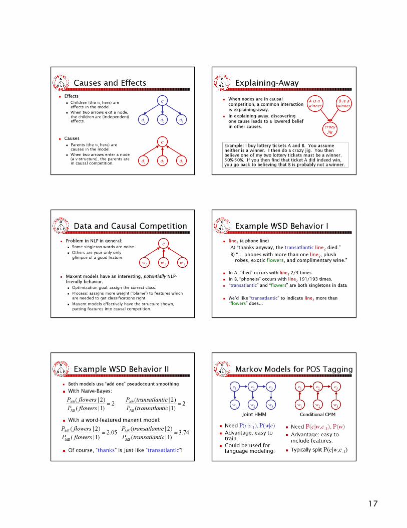
C a u s e s a n d E f f e c t s� Effects
� Children (the wi here) a re ef f ec ts in the m o del.� W hen tw o a rro w s ex it a no de,
the c hildren a re (indep endent) ef f ec ts .
� C a u ses� P a rents (the wi here) a re causes in the model.� W hen tw o ar r ow s enter a node
( a v -str uctur e) , the p ar ents ar e in causal comp etition.
c
d1 d2 d3
c
d1 d2 d3
Explaining-A w ay� When nodes are in causal
com p et it ion, a com m on int eract ion is ex p laining -aw ay .
� I n ex p laining -aw ay , discov ering one cause leads t o a low ered b elief in ot her causes. crazy
j i g
A i s a w i n n e r
B i s aw i n n e r
E x am p le: I b uy lot t ery t ick et s A and B . Y ou assum e neit her is a w inner. I t hen do a craz y j ig . Y ou t hen b eliev e one of m y t w o lot t ery t ick et s m ust b e a w inner, 5 0 % -5 0 % . I f y ou t hen f ind t hat t ick et A did indeed w in, y ou g o b ack t o b eliev ing t hat B is p rob ab ly not a w inner.
Data and Causal Competition� P rob lem in N L P in g eneral:
� Some singleton words are noise.� O th ers are y ou r only only
glimp se of a good f eatu re.
� Maxent m o d el s h av e an i nter es ti ng , potentially N L P -f r i end l y b eh av i o r .� O p timiz ation goal: assign th e c orrec t c lass.� P roc ess: assigns more weigh t ( “ b lame” ) to f eatu res wh ic h
are needed to get c lassif ic ations righ t.� M ax ent models ef f ec tiv ely h av e th e stru c tu re sh own,
p u tting f eatu res into c au sal c omp etition.
c
w1 w 2 w 3
Example WSD Behavior I� line2 ( a p h o ne line)
A) “thanks anyway, the transatlantic line 2 d ie d . ”B ) “ … p h o ne s w ith m o re th an o ne line 2 , p lu sh
ro b e s, e x o tic f lo w e rs, and co m p lim e ntary w ine . ”
� In A, “died” occurs with l ine2 2 / 3 tim es.� In B , “p hone(s)” occurs with l ine2 1 9 1 / 1 9 3 tim es.� “tra nsa tl a ntic” a nd “f l owers” a re b oth sing l etons in da ta
� W e’ d l ik e “tra nsa tl a ntic” to indica te l ine2 m ore tha n “f l owers” does. . .
Example WSD Behavior II� Both models use “add one” p seudoc ount smoothi ng� With Naïve-B ay es :
� With a w o r d -f eatu r ed m ax en t m o d el :
� O f c o u r s e, “ than k s ” is j u s t l ik e “ tr an s atl an tic ” !
2)1|()2|(=flowersP
flowersPNB
NB 2)1|()2|(=
tictransatlanPtictransatlanP
NB
NB
05.2)1|()2|(=flowersP
flowersPME
ME 74.3)1|()2|(=
tictransatlanPtictransatlanP
ME
ME
Markov Models for POS Taggingc1 c2 c3
w1 w2 w3
c1 c2 c3
w1 w2 w3
Joint HMM Conditional CMM
� Need P(c|w,c-1), P(w)� A dv a n t a g e: ea s y t o
i n c l u de f ea t u r es .� Typically split P(c|w,c-1)
� Need P(c|c-1), P ( w|c)� Advantage: easy to
tr ai n.� C ou l d b e u sed f or
l angu age m odel i ng.
18
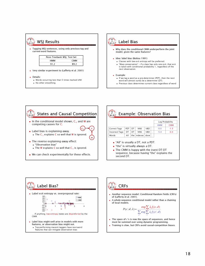
W S J R e s u l t s� Tagging WSJ sentences, using only previous-tag and current-w ord f eatures.
� V ery sim ilar ex perim ent to ( L af f erty et al. 2 0 0 1 )
� D etails:� Words occurring less than 5 times marked UNK� No other smoothing.
8 9 . 29 1 . 2C M MH M M
P enn Treeb ank WSJ, Test Set
L a b e l B i a s� Wh y d oes th e cond itional C M M und erperf orm th e j oint m od el, given th e sam e f eatures?
� I d ea: lab el b ias ( B ottou 1 9 9 1 )� Classes with low exit entropy will be preferred.� “ M ass preserv ation” – if a c lass has only one exit, that exit is tak en with c onditional probability 1 , reg ardless of the next observ ation.
� Example:� I f we tag a word as a pre-determ iner ( P D T ) , then the next word will alm ost su rely be a determ iner ( D T ) .
� P rev iou s c lass determ ines c u rrent c lass reg ardless of word
States and Causal Competition� In the conditional model shown, C-1 and W ar e
comp eting cau ses f or C.
� L ab el b ias is ex p laining -away .� The C-1 ex p l a i n s C s o w el l t ha t W i s i g n o r ed .
� T he r ev er se ex p laining -away ef f ect:� “ O b s er v a t i o n b i a s ”� The W ex p l a i n s C s o w el l t ha t C-1 i s i g n o r ed .
� We can check ex p er imentally f or these ef f ects.
c-1 c
w
Example: Observation Bias
� “All” is usually a DT, not a PDT.� “th e ” is v ir tually alw ays a DT.� Th e C M M is h ap p y w ith th e ( r ar e ) DT-DT
se q ue nc e , b e c ause h av ing “th e ” e x p lains th e se c ond DT.
Log Probability
.dovei n dex est h eA l lW or ds-0 .3-5 .4.V B DN N SD TD TI n c or r ec t T a g s-1 .3-0 .0.V B DN N SD TP D TC or r ec t T a g sC M MH M M
Label Bias?� Label exit entropy vs. overproposal rate:
… i f a n y t h i n g , l ow -en t r op y s t a t es a r e di s p r ef er r ed b y t h e C M M .
� Label bias might well arise in models with more f eatu res, or observ ation bias might not. � Top-pe r f or m i n g m a x e n t t a g g e r s h a v e n e x t -w or d
f e a t u r e s t h a t c a n m i t i g a t e ob s e r v a t i on b i a s .
-0.8-0.6-0.4-0.2
00.20.40.60.8
0 1 2 3 4
H M MC M M
CRFs� A nother seq u enc e model: C onditional R andom F ields ( C R F s) of (Lafferty et al. 2001).
� A w h ole-s eq u en c e c on d i ti on al m od el rath er th an a c h ai n i n g of loc al m od els .
� T h e s p ac e of c ’ s i s n ow th e s p ac e of s eq u en c es , an d h en c e m u s t b e s u m m ed ov er u s i n g d yn am i c p rog ram m i n g .
� T rai n i n g i s s low , b u t C R F s av oi d c au s al-c om p eti ti on b i as es .
∑ ∑'
),'(expc i
ii dcfλ=),|( λdcP ∑
iii dcf ),(exp λ
19
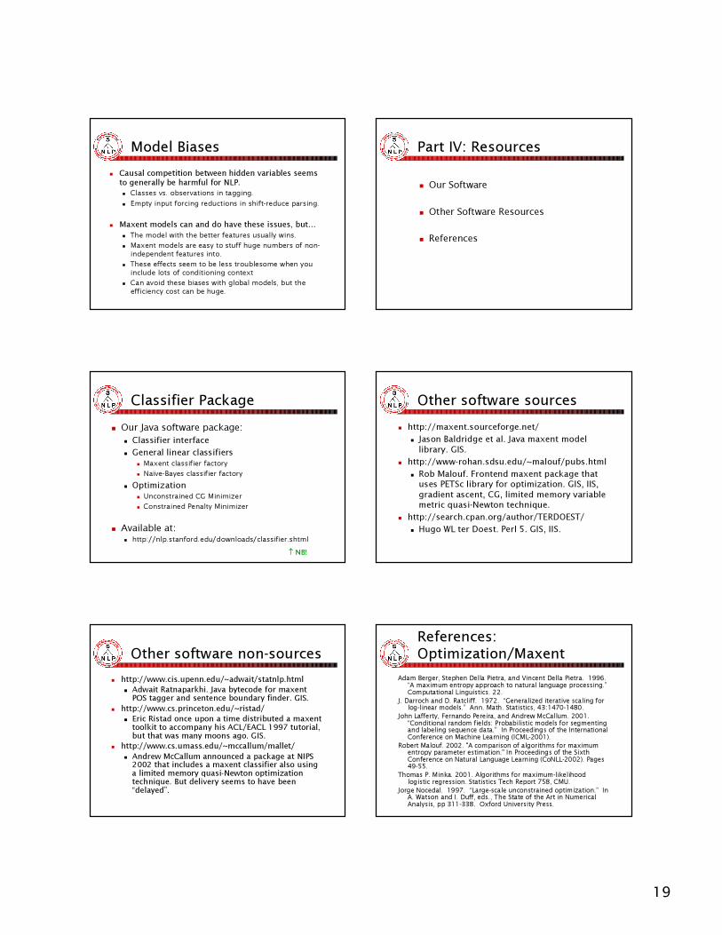
M o d e l B i a s e s� Causal competition between hidden variables seems
to g enerally be harmf ul f or N L P .� Classes vs. observations in tagging.� E m p ty inp u t f orc ing red u c tions in sh if t-red u c e p arsing.
� M ax ent models can and do have these issues, but…� T h e m od el w ith th e better f eatu res u su ally w ins.� M ax ent m od els are easy to stu f f h u ge nu m bers of non-ind ep end ent f eatu res into.
� T h ese ef f ec ts seem to be less trou blesom e w h en y ou inc lu d e lots of c ond itioning c ontex t
� Can avoid th ese biases w ith global m od els, bu t th e ef f ic ienc y c ost c an be h u ge.
P a r t I V : R e s o u r c e s
� Our Software
� Oth er Software R es ourc es
� R eferen c es
Classifier Package� Our J av a s oftware p ac k ag e:
� Classifier interface� G eneral linear classifiers
� Maxent c l as s i f i er f ac to r y� N aï v e-B ay es c l as s i f i er f ac to r y
� Optimization� U nc o ns tr ai ned C G Mi ni m i z er� C o ns tr ai ned P enal ty Mi ni m i z er
� Available at: � http://nlp.s ta nf o r d .e d u /d o w nlo a d s /c la s s i f i e r .s htm l
↑ NB!
Other software sources� http://m a x e n t.s o u r c e f o r g e .n e t/
� Jason B al d r i d g e e t al . Jav a m ax e nt m od e l l i b r ar y . G I S .
� h t t p : / / w w w -r oh an.sd su .e d u / ~ m al ou f / p u b s.h t m l� R ob M al ou f . F r ont e nd m ax e nt p ac k ag e t h at
u se s P E T S c l i b r ar y f or op t i m i z at i on. G I S , I I S , g r ad i e nt asc e nt , C G , l i m i t e d m e m or y v ar i ab l e m e t r i c q u asi -N e w t on t e c h ni q u e .
� h t t p : / / se ar c h .c p an.or g / au t h or / T E R D O E S T /� H u g o W L t e r D oe st . P e r l 5 . G I S , I I S .
Other software non-sou rc es� http://www.c i s .u pe n n .e d u /~ a d wa i t/s ta tn l p.htm l
� Adwait Ratnaparkhi. J av a b y te c o de f o r m ax e ntP O S tag g e r and s e nte nc e b o u ndary f inde r. G I S .
� http: //www.c s .princ e to n.e du /~ ris tad/� E ric Ris tad o nc e u po n a tim e dis trib u te d a m ax e nt to o l kit to ac c o m pany his AC L /E AC L 1 9 9 7 tu to rial , b u t that was m any m o o ns ag o . G I S .
� http: //www.c s .u m as s .e du /~ m c c al l u m /m al l e t/� Andre w M c C al l u m anno u nc e d a pac kag e at N I P S 2 0 0 2 that inc l u de s a m ax e nt c l as s if ie r al s o u s ing a l im ite d m e m o ry q u as i-N e wto n o ptim iz atio n te c hniq u e . B u t de l iv e ry s e e m s to hav e b e e n “ de l ay e d” .
References: O p t i m i z a t i o n/ M a x ent
Adam Berger, Stephen Della P i etra, and Vincent Della P ietr a. 1 9 9 6 . “ A m ax im u m entr o p y ap p r o ach to natu r al lang u ag e p r o ces s ing . ” C o m p u tatio nal L ing u is tics . 2 2 .
J . Dar r o ch and D. R atclif f . 1 9 7 2 . “ G ener aliz ed iter ativ e s caling f o r lo g -linear m o dels . ” A nn. M ath . S tatis tics , 4 3 : 1 4 7 0 -1 4 8 0 .
J o h n L af f er ty , F er nando P er eir a, and A ndr ew M cC allu m . 2 0 0 1 . “ C o nditio nal r ando m f ields : P r o b ab ilis tic m o dels f o r s eg m enting and lab eling s eq u ence data. ” I n P r o ceeding s o f th e I nter natio nal C o nf er ence o n M ach ine L ear ning ( I C M L -2 0 0 1 ) .
R o b er t M alo u f . 2 0 0 2 . " A co m p ar is o n o f alg o r ith m s f o r m ax im u m entr o p y p ar am eter es tim atio n. " I n P r o ceeding s o f th e S ix th C o nf er ence o n N atu r al L ang u ag e L ear ning ( C o N L L -2 0 0 2 ) . P ag es 4 9 -5 5 .
T h o m as P . M ink a. 2 0 0 1 . A lg o r ith m s f o r m ax im u m -lik elih o o d lo g is tic r eg r es s io n. S tatis tics T ech R ep o r t 7 5 8 , C M U .
J o r g e N o cedal. 1 9 9 7 . “ L ar g e-s cale u nco ns tr ained o p tim iz atio n. ” I n A . W ats o n and I . Du f f , eds . , T h e S tate o f th e A r t in N u m er ical A naly s is , p p 3 1 1 -3 3 8 . O x f o r d U niv er s ity P r es s .
20
R e f e r e n c e s : R e g u l a r i z a t i o nStanley Chen and Ronald Rosenfeld. A Survey of Smoothing
T ec hniq ues for M E M odels. IEEE Transactions on Speech and A u dio P rocessing , 8 ( 1 ) , p p . 3 7 --5 0 . J anuary 2 0 0 0 .
M . J ohnson, S. G eman, S. Canon, Z . Chi and S. Riez ler. 1 9 9 9 . E stimators for Stoc hastic “ U nific ation-b ased” G rammars. P roceeding s of A C L 1 9 9 9 .
R e f e r e n c e s : N a m e d E n t i t y R e c o g n i t i o n
Andrew B orthw ic k . 1 9 9 9 . A M ax imum E ntrop y Ap p roac h to N amed E ntity Rec ognition. P h.D . T hesis. N ew Y ork U niversity.
D an K lein, J osep h Smarr, H uy N guyen, and Christop her D . M anning. 2 0 0 3 . N amed E ntity Rec ognition w ith Charac ter-L evel M odels. P roceeding s the Sev enth C onf erence on N atu ral L ang u ag e L earning ( C oN L L 2 0 0 3 ) .
R e f e r e n c e s : P O S T a g g i n gJ ames R. Curran and Step hen Clark ( 2 0 0 3 ) . I nvestigating G I S and
Smoothing for M ax imum E ntrop y T aggers. P roceeding s of the 1 1 th A nnu al M eeting of the Eu ropean C hapter of the A ssociation f or C om pu tational L ing u istics ( EA C L ' 0 3 ) , p p .9 1 -9 8 , B udap est, H ungary
Adw ait Ratnap ark hi. A M ax imum E ntrop y P art-O f-Sp eec h T agger. I n P roceeding s of the Em pirical M ethods in N atu ral L ang u ag e P rocessing C onf erence, M ay 1 7 -1 8 , 1 9 9 6 . U niversity of P ennsylvania
K ristina T outanova and Christop her D . M anning. 2 0 0 0 . E nric hing the K now ledge Sourc es U sed in a M ax imum E ntrop y P art-of-Sp eec h T agger. P roceeding s of the J oint SIG D A T C onf erence on Em pirical M ethods in N atu ral L ang u ag e P rocessing and V ery L arg e C orpora ( EM N L P / V L C -2 0 0 0 ) , pp. 63-7 0 . H o n g K o n g .
K r i s t i n a T o u t a n o v a , D a n K l e i n , C h r i s t o ph e r D . M a n n i n g , a n d Y o r a mS i n g e r . 2 0 0 3. F e a t u r e -R i c h P a r t -o f -S pe e c h T a g g i n g w i t h a C y c l i c D e pe n d e n c y N e t w o r k . H L T -N A A C L 2 0 0 3.
References: Other A p p l i ca ti o ns
T o n g Z h a n g a n d F r a n k J . O l e s . 2 0 0 1 . T e x t C a t e g o r i z a t i o n B a s e d o n R e g u l a r i z e d L i n e a r C l a s s i f i c a t i o n M e t h o d s . I n f o r m a t i o n R e t r i e v a l 4 : 5 –31 .
R o n a l d R o s e n f e l d . A M a x i m u m E n t r o py A ppr o a c h t o A d a pt i v e S t a t i s t i c a l L a n g u a g e M o d e l i n g . C o m p u t e r , S p e e c h a n d L a n g u a g e1 0 , 1 8 7 --2 2 8 , 1 9 9 6.
A d w a i t R a t n a pa r k h i . A L i n e a r O b s e r v e d T i m e S t a t i s t i c a l P a r s e r B a s e d o n M a x i m u m E n t r o py M o d e l s . I n P r o c e e d i n g s o f t h e S e c o n d C o n f e r e n c e o n E m pi r i c a l M e t h o d s i n N a t u r a l L a n g u a g e P r o c e s s i n g . A u g . 1 -2 , 1 9 9 7 . B r o w n U n i v e r s i t y , P r o v i d e n c e , R h o d e I s l a n d .
A d w a i t R a t n a pa r k h i . U n s u pe r v i s e d S t a t i s t i c a l M o d e l s f o r P r e po s i t i o n a l P h r a s e A t t a c h m e n t . I n P r o c e e d i n g s o f t h e S e v e n t e e n t h I n t e r n a t i o n a l C o n f e r e n c e o n C o m pu t a t i o n a l L i n g u i s t i c s , A u g . 1 0 -1 4 , 1 9 9 8 . M o n t r e a l .
A n d r e i M i k h e e v . 2 0 0 0 . T a g g i n g S e n t e n c e B o u n d a r i e s . N A A C L 2 0 0 0 ,pp. 2 64 -2 7 1 .
References: L i ng u i sti c I ssu esL é o n B o t t o u . 1 9 9 1 . U n e a ppr o c h e t h e o r i q u e d e l ’ a ppr e n t i s s a g e
c o n n e x i o n i s t e ; a ppl i c a t i o n s a l a r e c o n n a i s s a n c e d e l a pa r o l e . P h .D . t h e s i s , U n i v e r s i t é d e P a r i s X I .
M a r k J o h n s o n . 2 0 0 1 . J o i n t a n d c o n d i t i o n a l e s t i m a t i o n o f t a g g i n g a n d pa r s i n g m o d e l s . I n A C L 39 , pa g e s 31 4 –32 1 .
D a n K l e i n a n d C h r i s t o ph e r D . M a n n i n g . 2 0 0 2 . C o n d i t i o n a l S t r u c t u r e v e r s u s C o n d i t i o n a l E s t i m a t i o n i n N L P M o d e l s . 2 0 0 2 C o n f e r e n c e o n E m pi r i c a l M e t h o d s i n N a t u r a l L a n g u a g e P r o c e s s i n g ( E M N L P 2 0 0 2 ) , pp. 9 -1 6.
A n d r e w M c C a l l u m , D a y n e F r e i t a g a n d F e r n a n d o P e r e i r a . 2 0 0 0 . M a x i m u m E n t r o py M a r k o v M o d e l s f o r I n f o r m a t i o n E x t r a c t i o n a n d S e g m e n t a t i o n . I C M L .
R i e z l e r , S ., T . K i n g , R . K a pl a n , R . C r o u c h , J . M a x w e l l a n d M . J o h n s o n . 2 0 0 2 . P a r s i n g t h e W a l l S t r e e t J o u r n a l u s i n g a L e x i c a l -F u n c t i o n a l G r a m m a r a n d D i s c r i m i n a t i v e E s t i m a t i o n T e c h n i q u e s . P r o c e e d i n g s o f t h e 4 0 t h A n n u a l M e e t i n g o f t h e A s s o c i a t i o n f o r C o m p u t a t i o n a l L i n g u i s t i c s .