Page 1
1
Miguel Vélez-Reyes1 and Aleksandar Stankovic2
1University of Puerto Rico-Mayagüez2Northeastern University
Challenges in Modeling and Identification of Power Systems: Dealing with Ill Conditioning, High Dimensionality, and other Challenges.
Page 2
2
Need for System Identification and Parameter Estimation
Operation of power systems near its limits leads to the need of having accurate models for
Operation Stability Analysis Control Power flow Reliability
Page 3
3
Motivation Model selection in many areas of engineering is
typically based on physical principles. Many of these models have a relatively large number of
parameters. Physical restrictions may not allow data collection for
parameter estimation based on experimental design. Measurements may not be rich enough to adequately
reflect the individual effects of all parameters. Distributed sensor networks allow us the observation of
spatio/temporal characteristics for power systems and other geographically distributed systems.
A vital issue in establishing utility of a model is whether parameters can be reliably identified from available experimental data.
Page 4
4
Problem of Interest #1 What model structures will give
us useful descriptions that will take full advantage of available data and be useful for the intended application
Gray Box models Physical + data driven modeling
Page 5
5
Dynamical Equivalents using NN
Consequences of deregulation – power systems that are more stressed, with participants less inclined to cooperate in overall power system control.
Increased reliance on 1) dynamical equivalents and 2) communication and computer technology to maintain stability.
Our research direction – generation and validation of dynamic equivalents directly from real-time measurements (and from locally available prior information)
Stankovic and Saric, ‘03
Page 6
6
New England/New York test power system
Retained subsystem
1
G153
G8
60
2625 28 29
61
G9
2427
30
9
8
3
18
17
2
4 14
15
21
16
57
19
20
G5
56
G4
58
G6
22
59
G7
23
1311
12
5
6
754
G255
G3
10
65
G13
37
G14
6640 48 47
41
G10
62
31 G1
1
63
32
33
38
46
G15
67
4249
36
64
G12
34
35
43
68
G16
52
50
51 45
44
39
ANN-based reduced-ordersubsystem
Interconnection and measu-rement points subsystem
Page 7
7
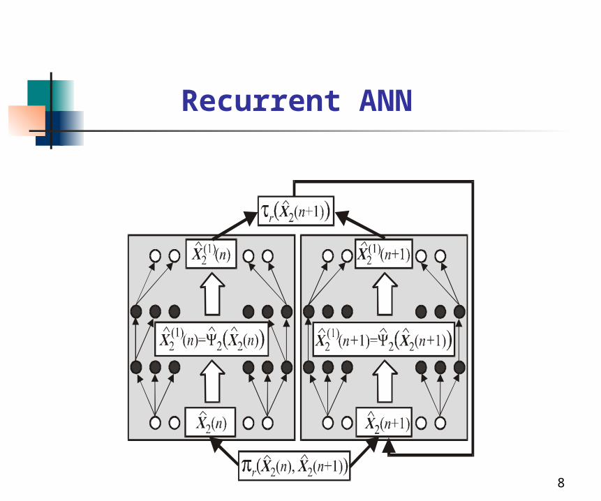
Bottleneck ANN Interface data
Interface data
Page 9
9
0 1 2 3 4 5 6 7 8 90.991
0.992
0.993
0.994
0.995
0.996
0.997
0.998
0.999
1
1.001
Gen
erat
or s
peed
(pu)
Time (sec)
Initial (DYNRED)Gray box (bottleneck ANN)Gray box (recurrent ANN)
0 1 2 3 4 5 6 7 8 9-2
-1.5
-1
-0.5
0
0.5
Act
ive
pow
er (p
u)
Time (sec)
Original systemGray box (bottleneck ANN)Gray box (recurrent ANN)
Equivalent generator speed in reduced subsystem.
Active power flow in interconnection 98.
Application
Page 10
10
Problem of Interest #2 Available data for parameter estimation
does not contain enough information about model parameters
Overparametrized models Poor quality of data
The resulting parameter estimation problem is ill-conditioned
Given a data set and a model for the system of interest what parameters can be reliably estimated from the data
Page 11
11
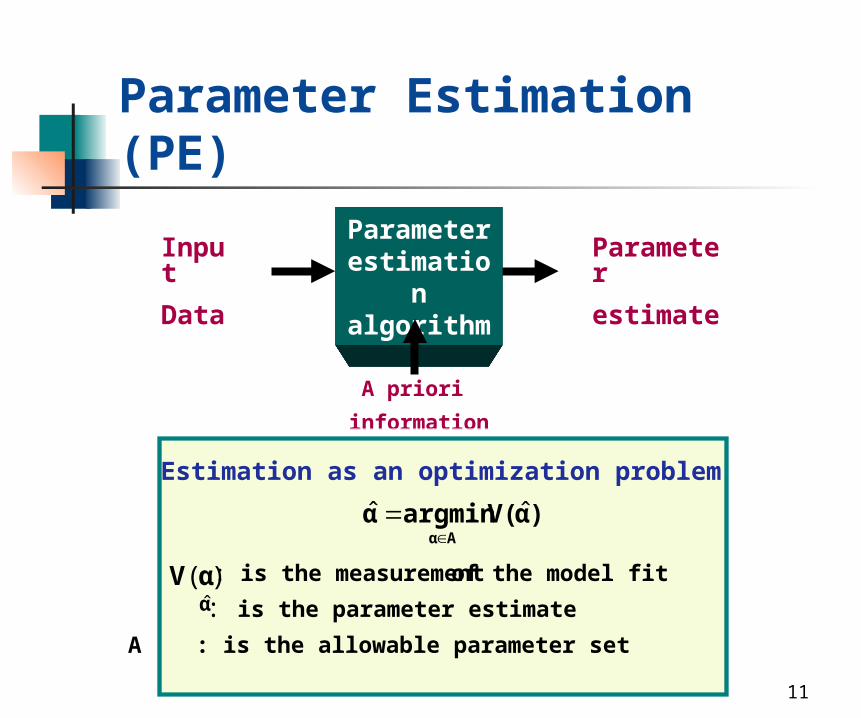
Parameter Estimation (PE)
Parameter
estimation
algorithm
Input
Data
Parameter
estimate
A priori
information
Estimation as an optimization problem
)(αV : is the measurementof the model fit
α : is the parameter estimate
A : is the allowable parameter set
)αV(argminαAα
ˆˆ
Page 12
12
Objectives
Develop metrics to diagnose ill- conditioning in a parameter estimation problem
Study how different formulations of the parameter estimation problem can be used to overcome ill-conditioning
Apply these techniques to parameter estimation problems
Page 13
13
Another Linear Example
Third column is noise plus columns 2 and 4 and b is the first column minus half of the second plus 0.01 times the third and fourth columns
A b
0.4919
, =
0.4249
- 0.1981
0.6291
- 0.7905
01112 0 5116 0 6234
0 5050 0 6239 0 5644 0 0589
0 5728 0 0843 0 6640 0 7480
0 4181 0 7689 0 9893 0 2200
. . .
. . . .
. . . .
. . . .
\ \
A b A b e
1.0000
- 0.5000
0.0100
0.0100
, =
0.8376
45.1105
- 45.5631
45.5513
Page 14
14
Quantifying Ill-Conditioning using Sensitivity Functions
Norm condition number
where J is the Jacobian of F at d. Componentwise condition number
dJd
ˆS
ˆ
d
dd
i
i
ˆ
d fˆ
S i
Page 15
15
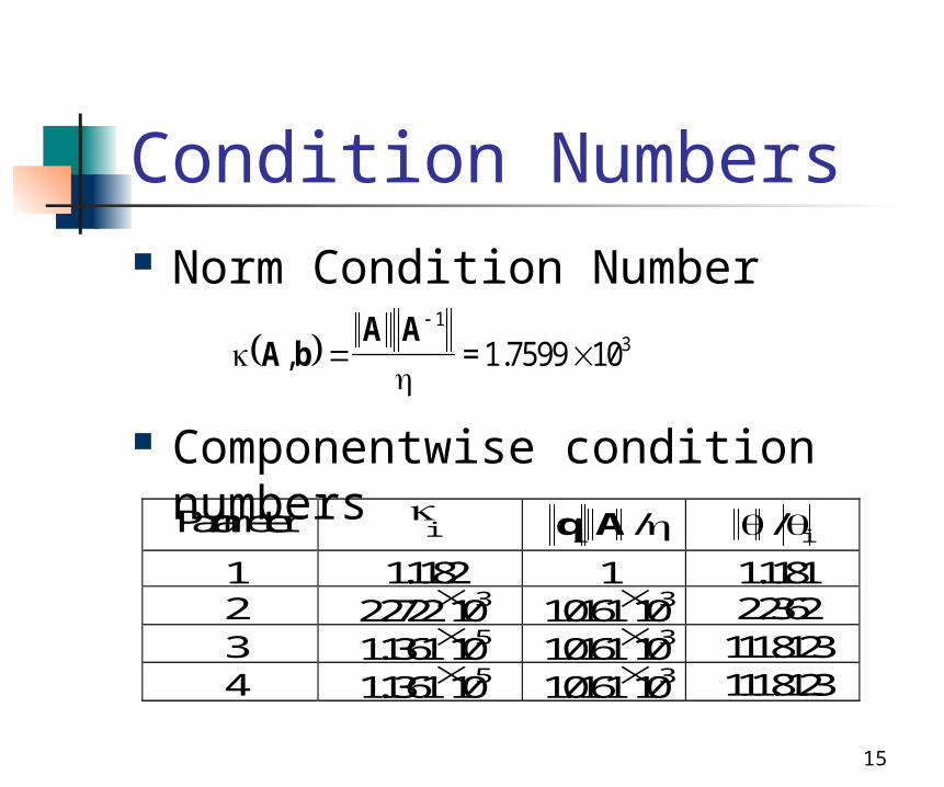
Condition Numbers Norm Condition Number
Componentwise condition numbersParameter
i q Ai / / i
1 1.1182 1 1.11812 2.2722103 1.0161103 2.23623 1.1361105 1.0161103 111.81234 1.1361105 1.0161103 111.8123
A bA A
, 1
= 1.7599 103
Page 16
16
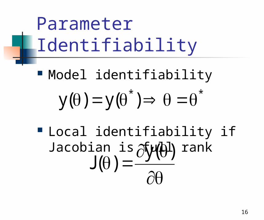
Parameter Identifiability Model identifiability
Local identifiability if Jacobian is full rank
)(y)(y **
)(y
)(J
Page 17
17
Nearness to Unidentifiability Clossedness to an unidentifiable
system is given by
Information about the rank structure of J() is contained in its SVD.
Jcond
1Jd
Page 18
18
SVD Analysis Jacobian for linear system is given by A Singular Values of A
1.7320 > 1.0000 > 0.9999 >>> 0.006 Numerical rank of A is equal to 3
Only three degrees of freedom Estimate only 3 parameters: Parameter subset
selection which ones? Parameters associated with the three
most independent columns of A will give the best solution from the sensitivity point of view (i.e. 1,2,4)
Bias versus sensitivity tradeoff
Page 19
19
Reduced-Order Problemwith 3=0
([ :,[ \
([ :,[ \
.
.
.
1 1
1 1
0 8376
0 4514
0 0106
2 4]) 2 4]
1.0000
- 0.4900
0.0200
,
2 4]) = 2 4]
A b
A b e
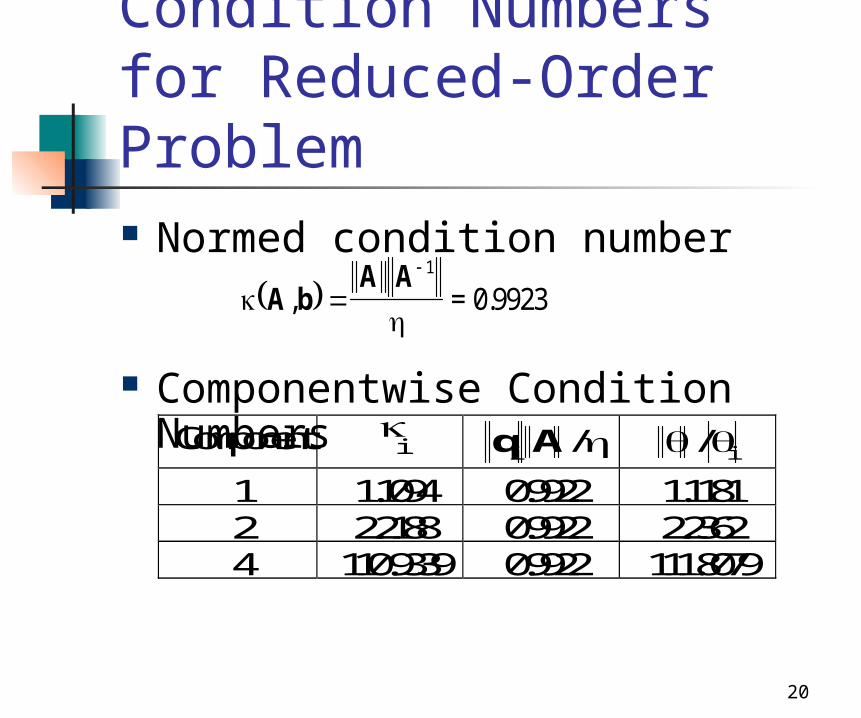
Page 20
20
Condition Numbers for Reduced-Order Problem Normed condition number
Componentwise Condition NumbersComponent
i q Ai / / i
1 1.1094 0.9922 1.11812 2.2188 0.9922 2.23624 110.9339 0.9922 111.8079
A bA A
, 1
0= .9923
Page 21
21
)(ˆ)( αyyαr
Noise
TunningMechanism
Output Error
++
+
-
u
y
)u(t)D()x(t)C(y(t)
)u(t)B()x(t)A((t)x
)(αy
SynchronousGenerator
Synchronous Motor Parameter Estimation
Fig. 1: Output Error Formulation
Page 22
22
Synchronous Machine
)ΔVE(x
1Δi
)ΔVE(x
1Δi
ΔVxT
xxΔE
xT
x
dt
Ed
ΔVT
kΔV
xT
xx
xT
xxE
xT
xx
xT
xx
T
1ΔE
TT
1
dt
Ed
ΔVT
kΔV
xT
xxΔE
xT
xxΔE
T
1
dt
Ed
d"d"
qq
q"q"
dd
d"q
"qo
"qq"
d"q
"qo
q"d
fd'do
q"d
"do
"d
'd
"d
'do
'dd"
q"d
"do
"d
'd
"d
'do
'dd
"do
'q'
do"do
"q
fd'do
q"d
'do
'dd"
q"d
'do
'dd'
q'do
'q
Where:
,T"
qo"qq
"do
'do
"d
'dd TxxkTTxxxα
fd
md
R
xk
Linearized Model
Page 23
23
Simulated Waveforms
Fig. 2 Field Voltage
Fig.3 Direct and Quadrature Voltages
Fig. 4 Direct and Quadrature Currents
Simulated waveforms with 0.5% of added noise
0.01
0 2 4 6 8 10 12 -0.03
-0.01
0
Time/sec
0 2 4 6 8 10 12
-0.02
0
0.02
0.03
0.04
0.05
0.06
0.07
q
ΔV
ΔV d
0 2 4 6 8 10 12 -3.5
-3 -2.5
2
-1.5 1
- 0.5 0
0.5 x 10 -4
Time/Sec
fdΔV
-0.15
-0.1
-0.05
0 2 4 6 8 10
12 -0.2
0
0.05
0.15
0.1
Time/sec
qi
di
Page 24
24
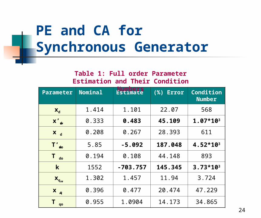
PE and CA for Synchronous Generator
Parameter Nominal Estimate (%) Error Condition Number
xd 1.414 1.101 22.07 568
x’d 0.333 0.483 45.109 1.07*103
x”d 0.208 0.267 28.393 611
T’do 5.85 -5.092 187.048 4.52*103
T”do 0.194 0.108 44.148 893
k 1552 -703.757 145.345 3.73*103
xq 1.302 1.457 11.94 3.724
x”q 0.396 0.477 20.474 47.229
T”qo 0.955 1.0904 14.173 34.865
Table 1: Full order Parameter Estimation and Their Condition
Numbers
Page 25
25
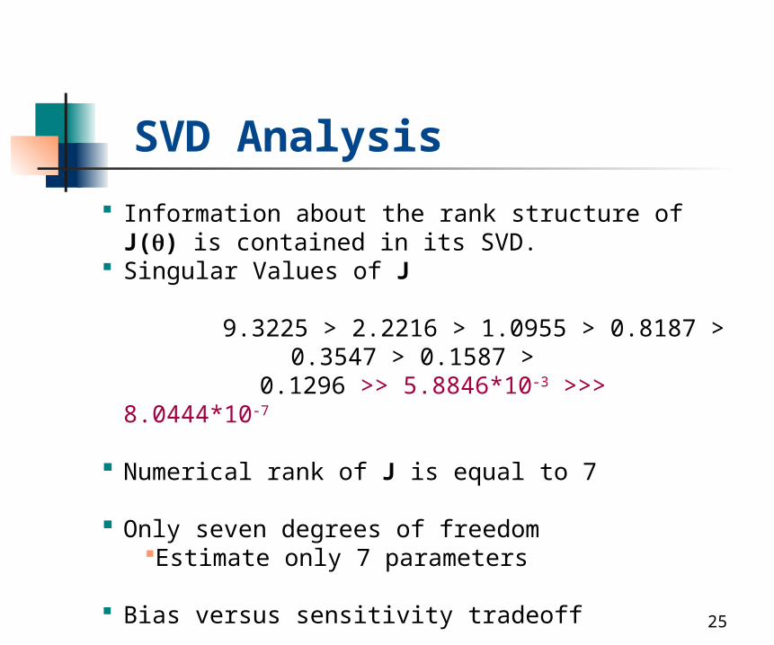
SVD Analysis Information about the rank structure of J() is
contained in its SVD. Singular Values of J
9.3225 > 2.2216 > 1.0955 > 0.8187 > 0.3547 > 0.1587 >
0.1296 >> 5.8846*10-3 >>> 8.0444*10-7
Numerical rank of J is equal to 7
Only seven degrees of freedomEstimate only 7 parameters
Bias versus sensitivity tradeoff
Page 26
26
Dealing with Ill-Conditioning
Regularization techniques Subset Selection (SS)
2
2
2
2)(ˆˆ *2
TIKH ααλ αyyargminα
Tikhonov Regularization (TR)
*22
T2
T1
ααs.tαyyargminα
)α(αα
2
2)(ˆˆ
Page 27
27
Subset Selection
From SVD analysis we know that there are two parameters to be fixed
Subset selection analysis gives the idea of which parameters to fix
Chose subset which results in best conditioning for the Jacobian.
x’d,k – Our Result xd, k – Our Result T’do, k – Selected by Burth (1999)
[1] M. Burth, G.C. Verghese, M. Vélez-Reyes “Subset Selection for Improved
Parameter Estimation in on-line Identification of a Synchronous Machine”,
IEEE Trans. on Power System. Vol14 1 pp. 218-225 March 1999
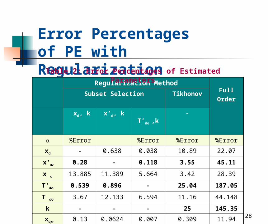
Page 28
28
Error Percentages of PE with Regularization
Regularization Method
FullOrder
Subset Selection Tikhonov
xd, k x’d, k T’do ,k -
%Error %Error %Error %Error
xd - 0.638 0.038 10.89 22.07
x’d 0.28 - 0.118 3.55 45.11
x”d 13.885 11.389 5.664 3.42 28.39
T’do 0.539 0.896 - 25.04 187.05
T”do 3.67 12.133 6.594 11.16 44.148
k - - - 25 145.35
xq 0.13 0.0624 0.007 0.309 11.94
x”q 0.538 0.555 0.04 0.241 20.47
T”qo 0.212 0.0505 0.0124 0.37 14.17
Table 2: Error Percentages of Estimated Parameters
Page 29
29
Conditioning Analysis with Regularization
Table 4: Condition Numbers with Regularization
Condition Numbers
Subset Selection Tikhonov
Full order
xd ,k x’d , k T’do , k -
xd - 3.311 2.731 161.86 568
x’d6.178 - 10.792 278.09 1.07*103
x”d99.82
6106.62 95.164 379.3 611
T’do4.156 8.80 - 113.88 4.52*103
T”do117 121.701 113 117.05 893
k - - - 10.499 3.73*103
xq3.724 3.724 3.724 3.7324 3.724
x”q47.22
2 47.222 47.222 47.02 47.229
T”qo34.86 34.86 34.86 35.073 34.865
α
Page 30
30
Comparison
0.37-35.073 -T’do
0.241-47.02 -k
0.3090.01243.7324 2.731xd
250.0410.499 113T”do
11.160.007117.05 95.164x”d
25.046.594113.88 10.792x’d
3.425.664379.3 47.229x”q
3.550.118278.09 34.864T’qo
10.890.0384161.86 3.724xd
NoneT’do,kNoneT’do,kfixed
TRSSTRSS
% ErrorCondition Number
Methodologies
Subset selection is the best but requires good prior estimates.
In Tikhonov Regularization some initial guess is required but estimate all parameters.
Table 5: Result of Comparisons
Page 31
31
Comments
Local sensitivity analysis provide reasonable metrics to determine the parameter conditioning.
Parameters associated with the direct axis were the worst conditioned
Parameter estimated error were reduced by using regularization
Sensitivity was significantly reduced by regularization
Different formulations to deal with ill-conditioning give different results with different information requirements.
Best Performance overall was for subset selection Initial Guess Number of parameters to estimate
Page 32
32
Some Challenges WE NEED NEW ALGORITHMS
THAT CAN TACKLE NONLINEAR, COMPLEX AND LARGE-SCALE PROBLEMS
WE NEED INTEGRATED APPROACHES FOR DATA MANAGEMENT, MODELING, SOLUTION, ANALYSIS AND VISUALIZATION
Page 33
33
Conclusions
“...While it is hard to predict the future, creating it is much easier…”
“...While it is hard to predict the future, creating it is much easier…”
We have an exciting opportunity to shape an integrated approach to merging models and data
G.J. McRae, MIT Course 10
Page 34
34
Acknowledgements Alex’s work ECS-9820977 Miguel’s work ECS-9702860