90
biglogo.gif (GIF Image, 800x418 pixels) http://matnmr.sourceforge.net/pics/biglogo.gif 1 of 1 12/06/06 05:47 PM

biglogo.gif (GIF Image, 800x418 pixels) http://matnmr.sourceforge.net/pics/biglogo.gif
1 of 1 12/06/06 05:47 PM
matNMR Manual Page: Navigation file:///home3/jabe/matlab/matNMRSourceCode/WebPages/manual/navigate...
1 of 3 02/28/07 05:48 PM
To go to the matNMR project page at source forge:
To go to the source forge homepage:
To go back to the matNMR page:
Search the manual pages directly
1 How to read this manual ? 1.1 Which parts should I read?
2 Installing matNMR 2.1 Installing matNMR 2.1.1 UNIX 2.1.2 MS Windows/MAC 2.2 Setting up matNMR (Options) 2.2.1 General options 2.2.2 Colour scheme settings 2.2.3 Screen settings 2.2.4 Font list 2.2.5 Line properties 2.2.6 Text properties
3 MATLAB and matNMR 3.1 MatNMR and the workspace 3.2 Input expressions 3.3 Important variables 3.4 Where is the NMR? 3.5 matNMR format for spectra 3.6 GUI and MATLAB 3.7 Memory usage 3.8 MATLAB and WYSIWYG
4 Processing in matNMR 4.1 Processing spectra with matNMR 4.2 1D, 2D and 3D mode 4.3 Using the processing history 4.4 Using macro's 4.5 Multi-window matNMR 4.6 Using short-keys 4.7 Apodizing FID's 4.8 Fourier transform 4.9 Phasing spectra

matNMR Manual Page: Navigation file:///home3/jabe/matlab/matNMRSourceCode/WebPages/manual/navigate...
2 of 3 02/28/07 05:48 PM
4.10 Baseline correction
5 The main window 5.1 General appearance 5.2 The menubar 5.2.1 Stop matNMR 5.2.2 Files 5.2.3 1D Processing 5.2.4 2D Processing 5.2.5 Plot manipulations 5.2.6 History/Macro 5.2.7 Create Output 5.2.8 Options 5.2.9 Help 5.2.10 Clear functions 5.3 Fitting of CSA tensors (MAS) 5.3.1 General appearance 5.3.2 Buttons 5.3.3 Menubar 5.4 Fitting of CSA tensors (Static) 5.4.1 General appearance 5.4.2 Buttons 5.4.3 Menubar 5.5 Fitting of Diffusion Curves 5.5.1 General appearance 5.5.2 Buttons 5.5.3 Menubar 5.6 Peak Deconvolution 5.6.1 General appearance 5.6.2 Buttons 5.6.3 Menubar 5.7 Fitting of Quadrupolar tensors 5.7.1 General appearance 5.7.2 Buttons 5.7.3 Menubar 5.8 Fitting of Relaxation Curves 5.8.1 General appearance 5.8.2 Buttons 5.8.3 Menubar
6 The 2D/3D Viewer 6.1 General appearance 6.2 The panel window 6.2.1 Contours 6.2.2 Mesh 3D 6.2.3 Stack 3D 6.2.4 Raster 2D 6.2.5 Tools 6.3 The menubar 6.3.1 Stop 2D/3D Viewer 6.3.2 Plot manipulations 6.3.3 History/Macro 6.3.4 Printing Menu 6.3.5 Copy figure 6.3.6 Options 6.3.7 Help 6.3.8 Clear functions
7 Producing output 7.1 Printing menu 7.2 Saving figures to disk 7.3 Using the Clipboard

matNMR Manual Page: Navigation file:///home3/jabe/matlab/matNMRSourceCode/WebPages/manual/navigate...
3 of 3 02/28/07 05:48 PM
8 Script-based processing
Search the manual pages directly

matNMR Manual Page: Introduction file:///home3/jabe/matlab/matNMRSourceCode/WebPages/manual/ManualInt...
1 of 1 02/28/07 05:28 PM
Chapter 1 - How to read this manual ?This manual was first written for matNMR 2.6 (October 2000) and describes all features and concept of it. Subsequent releases have been incorporated into the manual. This
means that the version that can be found on the website belongs to the latest release of matNMR. I am well aware that this manual is quite limited. It does for example not havean index and it doesn't allow searching through it. If anyone feels up to improving it, then please do so and send me the result!
The manual is divided in several chapters focussed around some subjects. For all features the actions required to perform it and also the implementation are described (inshort). The description of the implementation shall contain more information about what is done to a spectrum and how matNMR works. In most cases there will be noexplanation of standard MATLAB commands or features; the user is referred to the MATLAB documentation then. Also no explanations will be given for typical NMR operations asthese can be found relatively easy in the NMR literature.
In many occasions there will be spoken of "The main window" and the "2D/3D Viewer". These are the two main windows in matNMR. The first is used for processing while thesecond is used mainly for displaying and analysis. They can be started independently from the MATLAB command line by typing "nmr" or "nmr2d" respectively. Moreinformation about these windows is given in chapter 5, "The main window" and chapter 6, "The 2D/3D Viewer"
In the manual there will be made no clear distinction between an FID, a spectrum or a matrix. MATLAB does not care about the NMR behind a spectrum as it only knowsmatrices and vectors (for more information see paragraph 3.4, "Where is the NMR?"). Therefore whenever it says "FID" or "spectrum" in this manual it could just as well say"matrix" because in the end they're all the same thing.
1.1 Which parts of this manual should I definitely read ?
MatNMR can in principle be used as an independent processing program, just like any other package, making knowledge of MATLAB not really necessary. To use all itsfeatures to the fullest however one needs to know some things about it. These things are explained in chapter 3, "matNMR and MATLAB". There the interaction of matNMR and MATLAB is described in some detail. Even when you don't intend to do fancy stuff however I strongly advise you to read this chapter!
Also I advise you to read Chapter 4, "Processing in matNMR". This explains how processing in matNMR is thought to be done. Also things like using the processing history andmacro's effectively are explained in more detail here.
The installation of matNMR is explained in chapter 2, "Installing matNMR". How to configure matNMR to your personal likings is described in paragraph 2.2, "Setting up matNMR (options)".
Finally for people who don't want to use the matNMR user interface Chapter 8 , "Offline Processing with matNMR" explains how to use the processing capabilities inuser-defined scripts.
matNMR Manual Page: Installation file:///home3/jabe/matlab/matNMRSourceCode/WebPages/manual/Installati...
1 of 6 02/28/07 05:12 PM
Chapter 2 - Installing matNMR
2.1 Installing matNMR
Installing matNMR only requires copying the files into a directory and setting the search path variable such that it can find it. There are however some small differencesbetween UNIX systems and Windows/MAC systems. For both the preferred way of installation is described below.
2.1.1 UNIX
To install matNMR for a single user only on a UNIX system one must first extract the downloaded code into any directory. Here I will use '/home/jabe/matlab/matNMR' as anexample. Then one must change or create the file ~/matlab/startup.m. Specifically, the PATH variable needs to be changed so that MATLAB looks in the directory in which youhave just extracted the source code. This is a possible syntax to change the path:
path('/home/jabe/matlab/matNMR', path);
No further actions should be needed.
To install matNMR globally (i.e. for all users) on a UNIX system it is easiest to add a directory called matNMR to the matlabroot/toolbox directory (note that one needs theproper rights to do this, usually super user). Then extract the downloaded code into this directory. You then need to edit the matlabroot/toolbox/local/pathdef.m file. There youshould add the matlabroot/toolbox/matNMR directory to the list of standard directories.
In the matNMR directory there is a file called matnmroptions.mat and this is the configuration file for matNMR. If users have not copied this file into their personal matlabdirectory ~user/matlab then these settings will be used by matNMR. Note that users usually don't have permission to overwrite this file and therefore not change their settings!For more information on this see paragraph 2.2 "Setting up matNMR (Options)".
2.1.2 Windows / MAC
To install matNMR on a Windows or Macintosh system it is easiest to add a directory called matNMR to the matlabroot\toolbox directory. Then extract the downloaded codeinto this directory. To make matNMR generally available to all users you need to edit the matlabroot\toolbox\local\pathdef.m file. There you should add thematlabroot\toolbox\matNMR to the list of standard directories.
In the matNMR directory there is a file called matnmroptions.mat and this is the configuration file for matNMR. As users usually do not have a user-specific matlab directory(as on UNIX) all users will use the same configuration file. Only if the system can be set up such such that in the pathdef.m a user-specific matlab directory is specified, it can beavoided that all users use the same configuration file. If such a setup is present then users can copy the matnmroptions.mat into their personal matlab directory and have apersonal configuration. Note that it is necessary to have the personal matlab directory before the (general) matNMR directory for this to work! How to change the settings isdescribed below.

matNMR Manual Page: Installation file:///home3/jabe/matlab/matNMRSourceCode/WebPages/manual/Installati...
2 of 6 02/28/07 05:12 PM
2.2 Setting up matNMR (Options)
Several user-defined settings can be stored in matNMR, e.g. screen size, UI font size, the fonts the matNMR recognizes, line properties, text properties etc. All these are storedin the file matnmroptions.mat. When matNMR is started it will determine the location of this file and subsequent saving of the settings will be done to this location.
To configure matNMR to your liking start up the main window with "nmr" from the MATLAB prompt. In the resulting window you will find the "Options" in the menubar. Clickingthe mouse pointer on this menu will show a list of possible settings that can be changed:
-General Options-Colour scheme settings-Screen settings-Font List-Line properties-Text properties-Restore Defaults
In all of these menus changes of settings are applied either immediately or after pressing the "EXECUTE" button. Without saving these changes they only apply for thissession. The next session will then use the default parameters again as saved in the matnmroptions.mat file. Selecting the "Restore Defaults" will change all settings back totheir default values.
2.2.1 General Options
The general options menu is used to set some general working parameters. These include:

matNMR Manual Page: Installation file:///home3/jabe/matlab/matNMRSourceCode/WebPages/manual/Installati...
3 of 6 02/28/07 05:12 PM
-whether to show a logo during startup (general) -whether to ask for confirmation when closing a window (general) -How many processing steps may be undone in 1D mode -How many processing steps may be undone in 2D mode (Beware of memory usage) -whether to plot a x-scale by default (main window) -whether to plot a y-scale by default (main window) -which menus to show on startup (main window) - 1D / phase / 2D menus -whether to use an absolute or a relative(0-1) y-scale by default (main window) -whether to plot a grid by default (main window) -whether to multiply the first point of the FID by 0.5 by default -what type of FFT is used in TD2 by default (main window) -what type of FFT is used in TD1 by default (main window) -what default axes should be used for the time and frequency domains in both dimensions, see also paragraph 3.4 Where is the NMR (main window) -how many contour levels to use by default (2D/3D Viewer) -the default lower contour level limit (2D/3D Viewer) -the default upper contour level limit (2D/3D Viewer) -whether to use positive, negative, etc contours by default (2D/3D Viewer) -the default azimuth angle for a mesh plot (2D/3D Viewer) -the default elevation angle for a mesh plot (2D/3D Viewer) -the default azimuth angle for a 3D stack plot (2D/3D Viewer) -the default elevation angle for a 3D stack plot (2D/3D Viewer) -the default colormap in the 2D/3D Viewer -the default page orientation for printing -the default paper size for printing
2.2.2 Colour Scheme Settings

matNMR Manual Page: Installation file:///home3/jabe/matlab/matNMRSourceCode/WebPages/manual/Installati...
4 of 6 02/28/07 05:12 PM
This menu is used to define the colour scheme used in all matNMR windows. Several schemes have been pre-defined from which it is easy to make changes, if necessary.After changing values the results button will change, although for a complete overview of the effect matNMR must unfortunately be restarted. You MUST save the colour scheme
matNMR Manual Page: Installation file:///home3/jabe/matlab/matNMRSourceCode/WebPages/manual/Installati...
5 of 6 02/28/07 05:12 PM
before restarting matNMR! Note that this manual only shows the classic colour scheme.
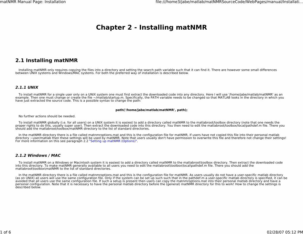
2.2.3 Screen Settings
This menu is used to define the screen sizes of the three main matNMR windows and also the font size that is used for UIcontrols. The numbers denote the size of the windowsin relative units, i.e. they range from 0 to 1. Changes are applied immediately (just be sure to press "ENTER" after changing a value!).
2.2.4 Font List
The font list menu species the list of fonts that matNMR recognizes. The default list in the downloaded code is based on a UNIX system which means many Windows/Macintoshfonts are not in this list! It is recommended to push the "import system fonts" button to create a list of fonts recognized on your system.
2.2.5 Line Properties

matNMR Manual Page: Installation file:///home3/jabe/matlab/matNMRSourceCode/WebPages/manual/Installati...
6 of 6 02/28/07 05:12 PM
The line properties hold for both the plots in the main window and the 2D/3D Viewer, i.e. for contour plots and 3D stack plots. This menu can but should not be used forchanging the appearance of single plots as all windows will be affected by this. For that the "Plot Manipulations" menu should be used instead.
2.2.6 Text Properties
The text properties hold for both the plots in the main window and the 2D/3D Viewer. This menu can but should not be used for changing the appearance of single plots as allwindows will be affected by this. For that the "Plot Manipulations" menu should be used instead.

matNMR Manual Page: MatNMR and MATLAB file:///home3/jabe/matlab/matNMRSourceCode/WebPages/manual/matNM...
1 of 5 02/28/07 05:29 PM
Chapter 3 - MATLAB and matNMR
3.1 MatNMR and the Workspace
One of the nice features of MATLAB is that it provides the user with a virtual workspace. It is basically memory that can be seen and manipulated from the MATLAB commandline. (e.g. the MATLAB who or whos commands can be used to see what variables are currently in your workspace) Any variable that is defined will be put in this workspace andcan at any time be manipulated again. Only variables that are used in functions have their own workspace. These cannot be accessed from the workspace and vice versa. Onlywhen defining a variable to be global one can use this subsequently in a function.
MATLAB allows for two ways of programming: scripts (m-file) or functions. (for more information please read the MATLAB documentation) The first will work in the sameworkspace as can be seen from the workspace, whereas the second will usually only produce an output to the workspace. MatNMR has been programmed as a script andtherefore ALL matNMR variables can be seen (AND manipulated!!) by the user. They are easy to recognize by the way as they ALWAYS start with a "Q"!
This has some consequences: -High flexibility because a user can invoke certain changes manually, thereby manipulating the output produced by matNMR. -Easy programming making user-additions to matNMR more easy. -A huge number of matNMR variables are seen by the user, making it more difficult to see the forest through the trees. -A risk of saving lots of unwanted matNMR variables to disk when trying to save something.
As the advantages strongly outweigh the disadvantages one just has to be careful when saving. Normally one can save all variables in the workspace by typing: save filename.matThis however will include all the matNMR variables which will increase the file size considerably. Therefore for saving some variables one either has to quit matNMR and thensave or specify the variables that need to be saved by typing: save filename.mat a b c d e f gor by using the "Save Spectrum to Disk" menus in the 1D and 2D processing menus from the main window menubar (See chapter 5, "The main window").
As a last remark: needless to say that the user must avoid using private variables that start with a "Q" as this may seriously affect matNMR!
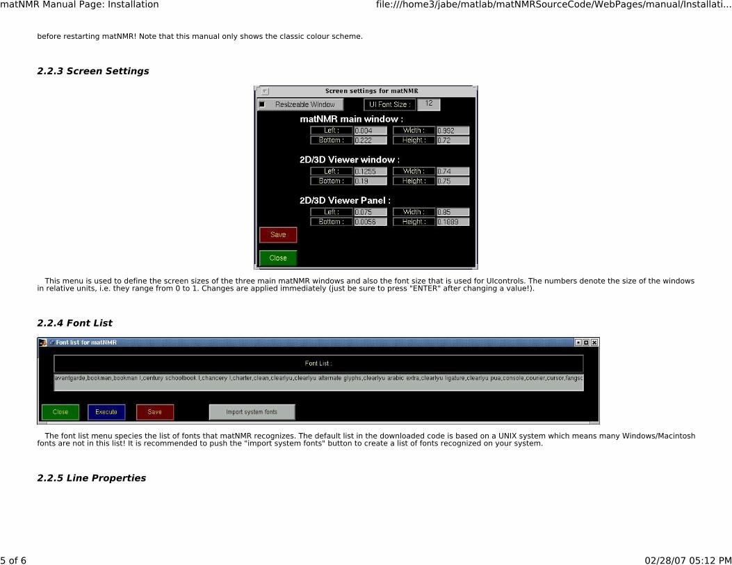
3.2 Input Expressions
Input in matNMR is usually done using either UI-controls from the main window and 2D/3D Viewer panel window OR using the standard input window:
matNMR Manual Page: MatNMR and MATLAB file:///home3/jabe/matlab/matNMRSourceCode/WebPages/manual/matNM...
2 of 5 02/28/07 05:29 PM
Whenever an edit button is used, i.e. a button in which one can write (for more information of different types of UI-controls please read the MATLAB documentation), theexpression is evaluated afterwards using the MATLAB eval command. This means that any general function that produces a result that is correct for the given input question,can be given as input. For example in the input window displayed above one can specify "Name" as: a (where a is a variable in the workspace)or a*10+4./b (where a and b are variables in the workspace)or 1:1024or diff((1.01).^(0:511)) (type "help diff" for more information on diff.m)etc ...
This again gives a lot of flexibility as the input format is free as long as the result is correct.
Note that the "full width" button allows expansion of the input window to the full width of the screen. This can be useful when the text written in the edit buttons is very long.
3.3 Important Variables
Currently, matNMR is written as a script (m-file) with a large pool of global variables that are used to keep track of all things. These global variables are visible in the workspaceas QmatNMR and QmatNMRsettings. Both are structures that contain many subitems. All items can be accessed in the usual way, i.e. QmatNMR.Spec1D will give the vectorcorresponding to the current 1D spectrum.
For most users it is not really necessary to know which variables are used by matNMR to do what. There are however a few variables of which it is probably not bad to knowwhat they do. Some of these will invariably show up eventually in some of the input windows and then it may be nice to know what they are there for. The following list shows afew important variables used when working with the main window:
Variable Name Usage in matNMR
Spec1D The current 1D spectrum
Axis1D The axis vector belonging to Spec1D
Size1D The dimension size of Spec1D
SW1D The spectral width of Spec1D in kHz
SF1D The carrier frequency of Spec1D in MHz
Spec2D The RR and RI parts of the current 2D spectrum (hypercomplex dataset)

matNMR Manual Page: MatNMR and MATLAB file:///home3/jabe/matlab/matNMRSourceCode/WebPages/manual/matNM...
3 of 5 02/28/07 05:29 PM
Spec2Dhc The IR and II parts of the current 2D spectrum (hypercomplex dataset)
AxisTD2 The axis vector belonging to TD2 of the current 2D spectrum
AxisTD1 The axis vector belonging to TD1 of the current 2D spectrum
SizeTD2 The dimension size of TD2 for the current 2D spectrum
SizeTD1 The dimension size of TD1 for the current 2D spectrum
SWTD2 The spectral width for TD2 of the current 2D spectrum in kHz
SWTD1 The spectral width for TD1 of the current 2D spectrum in kHz
SFTD2 The carrier frequency for TD2 of the current 2D spectrum in MHz
SFTD1 The carrier frequency for TD1 of the current 2D spectrum in MHz
Dim The current dimension (0=1D, 1=TD2, 2=TD1)
Fig The figure handle for the main window
History The processing history belonging to the current 1D OR 2D spectrum
HistoryMacro The processing macro belonging to the current 1D OR 2D spectrum
QFitResults Results from the last peak fitting. These are not stored in the QmatNMR structure! For more information on the format of this variable see paragraph 5.3.1,General appearance.
QSSAFitResults Results from the last MAS CSA fitting. These are not stored in the QmatNMR structure!
QCSAFitResults Results from the last static CSA fitting. These are not stored in the QmatNMR structure!
QQuadFitResults Results from the last quadrupolar-tensor fitting. These are not stored in the QmatNMR structure!
QDiffFitResults Results from the last diffusion-curve fitting. These are not stored in the QmatNMR structure!
QT1FitResults Results from the last relaxation-curve fitting. These are not stored in the QmatNMR structure!
As can be seen from the table there are different variables for 1D and 2D spectra. The distinction between working in 1D or in 2D mode is quite clear although it cannot beseen directly while working with matNMR. This is explained in more detail in paragraph 4.2, "1D and 2D mode".
A comparable list can be given for the 2D/3D Viewer window:
Variable Name Usage in matNMR
Spec2D3D The last plotted spectrum
Axis2D3DTD2 The axis vector belonging to TD2 of Spec2D3D
Axis2D3DTD1 The axis vector belonging to TD1 of Spec2D3D
PeakList The peak list belonging to Spec2D3D
History2D3D The processing history belonging to Spec2D3D
Fig2D3D The current 2D/3D Viewer window
AxisNR2D3D The current axis number (i.e. nr of subplot)
AxisHandle2D3D The axis handle belonging to AxisNR2D3D
3.4 Where is the NMR?
A big difference between working with matNMR and other NMR processing packages is that the user doesn't NEED to work with typical NMR parameters like spectral width,the carrier frequency, etc while processing. Naturally that comes from the fact that MATLAB doesn't know NMR, only matrices, vectors and numbers, and also matNMR doesn'tcare really about the NMR behind a FID, i.e. every axis plotted below a spectrum is given in points unless a different axis is defined.
Having said that, matNMR does show the typical NMR units if wanted and if the relevant parameters have been supplied correctly. If the spectral width and the spectral

matNMR Manual Page: MatNMR and MATLAB file:///home3/jabe/matlab/matNMRSourceCode/WebPages/manual/matNM...
4 of 5 02/28/07 05:29 PM
frequency for a certain dimension have been supplied (either during loading of a binary FID or manually, then the default axis, see also paragraph 2.2.1 General Options, will produce proper time and frequency axes (Hz or PPM). The reference for such frequency axes is always set to 0 and in the center of the spectrum. NOTE that by changing thespectral width and/or spectral frequency the default axis will change immediately.
There are two ways of properly referencing spectra: 1) defining and axis for a particular spectrum directly OR 2) by applying an external reference.1. Axis vectors can be defined from the (Plot Manipulations - ruler X-axis) menubar in the main window. The typical axes in PPM, Hz or time can be defined but also axes inpoints or other less typical axes can easily be defined (for more information on how to change the axis vector see paragraph 5.2.5, "Plot manipulations"). As the spectrum is just a numerical matrix it can be manipulated very easily during processing. The axis vectors are just used for plotting, but on the other hand:NOTE: whenever there is an input concerning coordinates they must usually be given in the unit of the axis vector! (e.g. for extracting parts of a spectrum, integrating, etc...)
2. An external reference may be loaded from external datasets, either as defined in a file on your spectrometer, or by using the reference as made in another variable inmatNMR. To use the values set on your spectrometer it is possible to import those values by using the "Import external reference" in the "Plot Manipulations" - "Ruler X-Axis" -"External reference" menus. MatNMR will then try and extract the values from other datasets on disk. Alternatively, you may define a fixed axis for a certain spectrum inmatNMR, as described above. Either by saving the external reference directly, or by storing the spectrum in the workspace those values may serve as an external reference.The "Apply external reference" item will ask for a variable containing an external reference, i.e. a spectrum OR a reference only, which may then be applied to the currentspectrum.
3.5 matNMR format for spectra
MatNMR can save spectra either as matrices into the workspace (or onto disk directly) or in the matNMR format. This matNMR format makes a structure of the variable withthe following fields:
VariableName.Spectrum VariableName.History VariableName.HistoryMacro VariableName.AxisTD2 VariableName.AxisTD1 VariableName.SweepWidthTD2 VariableName.SweepWidthTD1 VariableName.SpectralFrequencyTD2 VariableName.SpectralFrequencyTD1 VariableName.Hypercomplex VariableName.PeakListNums VariableName.PeakListText VariableName.FIDstatusTD2 VariableName.FIDstatusTD1
(for more information on structures and other MATLAB data types please read the MATLAB documentation)
The spectrum will appear in the workspace as a struct array under the name VariableName. Saving in this format thus allows for easy access to the NMR parametersbelonging to this spectrum. Note that for accessing the fields one needs to type "VariableName.FieldName" to obtain the proper result. As many functions will produce errormessages when supplying them with the matNMR structure directly, it is important to realize of what type a certain variable is.
3.6 GUI and MATLAB
MatNMR is fully GUI (graphical user interface) programmed. Being able to do this is a nice feature of MATLAB but it is not 100% perfect. Especially when clicking the mousevery fast onto several objects can be the cause of many problems. The problem can often be traced back to the code that is run (bad programming). Often however such

matNMR Manual Page: MatNMR and MATLAB file:///home3/jabe/matlab/matNMRSourceCode/WebPages/manual/matNM...
5 of 5 02/28/07 05:29 PM
problems arise from the fact that the MATLAB command line parser is slower than the mouse pointer. When using functions like gcf, gca and gco (get current figure, get currentaxis and get current object respectively) problems can occur because the current object is not the object that the code intended to work on. Therefore a word of caution must begiven: don't overdo it, don't try and be the fastest mouse-clicker on earth when working with MATLAB.
3.7 Memory usage
As matNMR does all processing in memory the memory usage can be quite considerable. Especially so because MATLAB will only take continuous blocks of memory whencreating a new variable. This means that when it cannot find a block in the currently taken memory of the proper size it will ask for more memory. On a UNIX system this caneasily lead to memory usage of 256Mb when processing a 2048x2048 sized spectrum. Under Windows this seems to be less of a problem though. Anyway, it is important to beaware of how much memory is in use and if necessary to stop MATLAB every once in a while, just to free the memory again.Note, starting from version 2.7 matNMR has an optional undo function. Although very useful to have, this function may indeed induce massive memory usage if too many undosteps are allowed as the full matrices are stored for each step. More information on the undo function may be found in paragraph 5.2.11, "Goodies".
3.8 MATLAB and WYSIWYG
Unfortunately MATLAB in general is not a "what you see is what you get"-kind of program (WYSIWYG). Neither is matNMR therefore. For versions of matNMR older than 2.6(march 2001) this calls for some improvisation if you really want to use matNMR to create nice plots. The axes, and therefore the spectra, are always plotted at their correctpositions. The problem mostly lies with the fonts. For some reason they are not scaled in the same way as the axes. Especially the positioning of floating text, e.g. the super titlein the 2D/3D Viewer, must be checked in the resulting plot. In principle it therefore advised to plot to a file on disk first before sending it to a printer.For matNMR 2.6 (march 2001) and newer an option has been added to the printing menu: "enforce WYSIWYG". This tries to ensure WYSIWYG behaviour but it still isn't perfect.The routine works fine as long as the absolute size of the window is not bigger than the paper size. Upon rescaling the window and all its objects and fonts again there is aproblem with the fonts in some cases. The best thing to do then is to resize the window manually and make sure that the printing routine does not need to rescale it. A warningmessage concerning this point will be given by the printing routine though. For more information on how to output plots see chapter 7, "Producing output".
matNMR Manual Page: Processing file:///home3/jabe/matlab/matNMRSourceCode/WebPages/manual/Processi...
1 of 8 11/23/07 06:01 PM
Chapter 4 - Processing with matNMR
4.1 Processing spectra with matNMR
Like any other program matNMR requires a certain sequence of events to be followed for properly processing spectra. In general it can be said that everything is done stepwise. Althoughprocessing macro's can be defined (see paragraph 4.4, "Using macro's") there are no all-in-one processing steps pre-defined. As an example two typical sets of processing actions are shownbelow, one for a 1D and one for processing a 2D spectrum. In general for 1D spectra the routine will be something like :
load 1Denter spectral width (optional)select a proper apodization functionset size 1Dchoose Fourier Mode (Optional --> is set by default options)FT 1Dadjust phasesave spec 1D
For a 2D this basically looks the same but it needs some steps more. This is because certain steps (like phasing and apodizing) assume working on a 1D spectrum and unless matNMR isinstructed to work on the whole 2D matrix only the 1D spectrum in the current view is affected. (For more information see paragraph 4.2, "1D, 2D and 3D mode"). Therefore it is important not to forget the "Apodize 2D" and "Set Phase 2D" commands during processing.Typically processing a 2D will look like :
load 2Dchoose Fourier Mode (Optional --> is set by default options)enter spectral width of TD 2 (optional)select a proper apodization function for TD 2Apodize 2D (to apodize the whole 2D matrix !!)set size 2D (Only for TD 2 --> keeping TD 1 small makes the FT and phasing faster !!)FT 2Dadjust phase for the first rowSet Phase 2D (to set the phase for the whole 2D spectrum !!)get column (depends on where the signal is)select a proper apodization function for TD 1choose Fourier Mode (Optional)enter spectral width of TD 1 (optional)Apodize 2D (to apodize the whole 2D matrix !!)set size 2D (Only for TD 1)FT 2Dadjust the phase for TD 1Set Phase 2D (to set the phase for the whole 2D spectrum !!)
and if needed:
adjust the phase for TD 2Set Phase 2D (to set the phase for the whole 2D spectrum !!)Baseline correction

matNMR Manual Page: Processing file:///home3/jabe/matlab/matNMRSourceCode/WebPages/manual/Processi...
2 of 8 11/23/07 06:01 PM
4.1.1 Practical Tutorial
As a practical example is the easiest way to learn about matNMR, there are two datasets included in the matNMR distribution. These can be found in a subdirectory called "Examples", inthe directory where you have stored matNMR. The datasets are solid-NMR spectra generated with Spinsight. They are called "SpinsightExample1" and "SpinsightExample2".
Loading the data into the Matlab workspace:
In this case there are two ways of importing the two datasets into Matlab: separately or as a series. To load them separately go into the "files" menu and select "binary FID". Select thefile that contains the FID. For Spinsight data this file is always called "data". After selecting this file, an input window comes up. In this window the size of the data must be specified, thename of the variable in the Matlab workspace must be defined, and the format of the data must be specified. When the standard parameter files are present (i.e. the full dataset and not justthe FID) then the sizes will be deduced from those files. The data format is in some cases recognized automatically. Finally, when the dataset should not only be stored in the workspace butalso loaded into matNMR directly then select the flag.
Since the two datasets are both Spinsight datasets and have a very similar name, they can also be loaded as a series of binary FIDs. Select the appropriate entry in the "files" menu.Select the file that contains the FID. In the input window you can define as common part of the file name, e.g. "/home/jabe/matlab/matNMR/Examples/SpinsightExample$#$/data" and arange "1:2". Here, the "$#$" is used as a code that is substituted once by All elements in the numerical range. Otherwise everything else is the same as above. Clicking OK will load bothdatasets in one go.
Processing the 1D dataset, SpinsightExample1:
From the main window, press button "load 1D" in the 1D menu, or go to the "1D Processing" menu. Use the name of the variable in the workspace that contains the data for example 1.Load the data as an FID. To process the spectrum use e.g.
Hamming apodization (phase factor 0).Set the size to 2k points. Do a "complex FT", with or without multiplying the first point by 0.5.Use the mouse to apply -2.1 degrees zeroth-order phase correction, or type -2.1 in the appropriate edit button (press or mouse mouse pointer out of window to activate).To perform a baseline correction, go into the "1D Processing" menu and select "standard processing" and "baseline correction". Use "Define peaks" to exclude the area of the signalfrom the baseline fit. (left-click=define, right-click=stop). A polynomial of order 0, 1, or 2 should be fine in this case.Store the processed spectrum in the workspace by using the "Add to workspace" button.Alternatively, you may only store the processing actions with the FID (for large 2D spectra often smaller than storing the spectrum. In that case go into the "History / Macro" menu andselect "Connect to FID". Supply the name that contains the example 1. For fun, reload the dataset, for example using the "reload last" button on the right of your screen. Go into the"History / Macro" menu and select "reprocess from history". This should reproduce the spectrum.
Processing the 2D dataset, SpinsightExample2:
From the main window, press button "load 2D" in the 2D menu, or go to the "2D Processing" menu. Use the name of the variable in the workspace that contains the data for example 2.Load the data as an FID. To process the spectrum use e.g.
This is a 2D dataset with STATES in the indirect dimension for phase sensitivity. The format is already as matNMR requires it to be. First the dataset in made into a hypercomplex set (2complex matrices). Use the "Start STATES processing" in the "2D Processing" menu.Add 40 Hz of Gaussian apodization. Make sure you use the "Apodize 2D" button to apply the apodization to the entire dataset!Set the size to 1k points in TD2 using the "set sizes" button in the 2D menu.Perform the FT in TD2. The FT mode should say STATES.Set the phase properly using the buttons. The reference for the first-order phase correction can be defined by clicking the "Reference Ph1" button. Use the crosshair to indicate theposition. Using a "reference ph1" of 776 (assuming 1k points in TD2!), phase values of 51 and -227 degrees for the zeroth and first-order corrections should yield an in-phase spectrumwith 4 lines.Check the position of the lines. These are useful for process the indirect dimension. Select the "Zoom" function and zoom into the left doublet. The use the "Get position" button toextract the position. Push the left button and move the mouse to follow the lines. The "X index" is the number you want to remember. Click on "Done".Repeat the previous for the right doublet in the spectrum. The indices should be e.g. 784 and 373.Go to column 784 by typing the number in the appropriate edit button in the windowBecause the pulse program did not conform to the default in Spinsight, the spectral width in TD1 could not be deduced. This was also shown in the Matlab command window (Pleaselook!), where it says that the dw2 parameter could not be found. Hence the spectral width must be supplied manually. Type 25 (kHz) in the edit button next to "Spectr. Width (kHz)".Use Hamming apodization with phase factor 0. Make sure you use the "Apodize 2D" button to apply the apodization to the entire dataset!Set the size to 1k points in TD1 using the "set sizes" button in the 2D menu.Perform the FT in TD1. The FT mode should say STATES. This should show the same 4 lines as before, but reversed.Because the STATES modulation in the pulse program was not of the correct sign, the spectrum in TD1 is reversed, compared to TD2. To correct this use the "Flip L/R" in the "2Dprocessing"+"standard processing" menu.Now the phase correction can be perfected: select row 784. Set the zero-order phase correction on the most left peak. Set the reference for ph1 on this peak. Select row 373. Adjust thefirst-order phase correction on the most right peak in the spectrum. Apply the phase to the entire spectrum ("Set Phase 2D"). Do the same in TD1.Select row 784 and go into the "2D Processing" menu, "standard processing", and select "baseline correction". use the "define peaks" to exclude the 4 signals fromthe baseline fit anduse a first-order polynomial. Do the same for TD1.Store the spectrum in the workspace by using the "Add to workspace" button.
matNMR Manual Page: Processing file:///home3/jabe/matlab/matNMRSourceCode/WebPages/manual/Processi...
3 of 8 11/23/07 06:01 PM
View the spectrum using the 2D/3D viewer: push the appropriate button on the right side of the 2D menu. Make, for example, a contour plot by selecting relative contours.
4.2 1D, 2D and 3D mode
It is important to realize the difference between working on a 1D and on a 2D spectrum. In principle what is shown in the view, while processing a 2D spectrum, is a certain row or columnfrom the matrix. The variable QmatNMR.Dim denotes the current dimension in which we are working: 0=1D spectrum, 1=TD2, 2=TD1. For a certain row the QmatNMR.Dim will be set to 1(in a true 1D mode QmatNMR.Dim is set to 0). When changing the phase or apodizing, the current view is changed directly on the screen. The mode is not changed though and thereforeQmatNMR.Dim will still be either 1 or 2. However, the change is not imposed to the entire 2D matrix until the corresponding buttons "Set Phase 2D" and "Apodize 2D" are pushed!
Then there are several functions (Sum TD2, Sum TD1, Diagonal, etc) that operate on a 2D matrix and which have a 1D spectrum as output. In those cases the mode is switched to a true1D mode (QmatNMR.Dim=0). This is important to realize, e.g. when doing baseline correction: It is often convenient to look at the sum over a certain dimension to see where the intensitiesare in the spectrum. However then the mode is switched to a 1D mode and the 2D baseline correction routine doesn't know on which dimension to operate then (by default it will assume tobe working on TD2 for this tourine by the way).
Another way of switching the mode from 2D to 1D is by selecting a 1D function while processing a 2D spectrum. For example doing a 1D FFT will switch the current mode to 1D and do aFFT then. The 2D spectrum is not affected by this at all. (This can be also useful for checking certain processing steps as using 1D functions is usually faster than 2D functions.) To switchback to the 2D mode simply select a row or column from the matrix, using the appropriate UI-controls in the main window.
MatNMR does NOT offer full 3D processing capabilities but rather allows for efficient processing of series of similar 2D spectra, especially using processing macros. When working with 3Dmatrices in the main window a new window is openened from which an output variable must be declared. This is done in order to conserve memory usage: the 3D matrices are not copiedinto dedicated matNMR variables but changes to the input variable are stored directly in the output variable. The first dimension of the 3D matrix is the index of the spectrum, whilst thesecond and third dimension stand for TD1 and TD2 respectively.
This feature is particularly useful for processing sets of simulations. Subsequent plotting of these sets of spectra is facilitated by the 2D/3D viewer support for 3D matrices. Upon detectinga 3D matrix, the 2D/3D viewer will check the number of subplots in the figure window and will try and plot the set of 2D spectra into the available subplots. When combining this withplotting macro's, very efficient plotting of the data may be achieved. For more information on how to optimize the use of plotting macro's, see paragraph 4.4, "Using macro's".
4.3 Using the processing history
A relatively unique feature of matNMR is the processing history (only recently other packages have started to implement this). MatNMR keeps track of all actions during processing. Afterprocessing the spectrum is finished the history can be connected to the FID. When reloading the FID then into matNMR, the spectrum can be obtained by "Reprocessing from History", foundin the "History" menu of the menubar in the main window. This has some nice advantages:
-No need to write down processing parameters as they are saved on disk -No need to save the spectrum to disk (which is usually much bigger than the FID -Easy and fast reprocessing of the FID afterwards
Connecting a processing history to an FID induces matNMR to convert the matrix in the workspace to the matNMR format. For more information about this see paragraph 3.5, "matNMR format for spectra". All necessary information can easily be accessed using this format. The peak list can also be connected to the FID making plotting the only step necessary afterreprocessing a spectrum.
History macros can also be converted into independent processing scripts on disk. The scripts can be applied to any dataset, the name of which is the input parameter of the script. Seealso Chapter 8, Script-based processing with matNMR.
At any time the processing history can be viewed as text in a separate window. The text is stored in the variable QmatNMR.History. At the same time however a numerical matrix is storedin the workspace, called QmatNMR.HistoryMacro, that contains the processing history as a matNMR macro. This is explained in more detail in paragraph 4.4 below.
matNMR Manual Page: Processing file:///home3/jabe/matlab/matNMRSourceCode/WebPages/manual/Processi...
4 of 8 11/23/07 06:01 PM
Now in principle can every processing step be reprocessed afterwards. Everything except creating a non-linear axis vector! Most axes have linear increments and therefore only the axisoffset and increments are saved into the processing history macro. Non-linear axes are not stored into it. This also means they will not be reproduced when reprocessing. It wouldn't beterribly difficult implementing this but it would increase the size of the macro considerably and is therefore not implemented currently.
More explanation on how to use the history can be found in paragraph 5.2.6, "History/Macro".
4.4 Using macro's
MatNMR allows for the definition of macro's from the menubar in the main window. Currently, both processing and plotting actions can be stored in a macro. Macro's in matNMR are justmatrices of numbers encoding for all processing steps. Besides adding general matNMR processing routine steps to a macro, user-defined commands may be defined as well. The commandstring for these commands will be translated into numbers and is stored as such in the history macro. After finishing recording the macro it can be saved as a normal variable in theworkspace (or on disk) for later use. Processing macro's can only be executed in the main window. Plotting macro's can be executed in any of the matNMR windows.
Note that plotting actions are not permanent and are usually all removed when matNMR updates a window. In case of the 2D/3D viewer plotting macro's can be defined in multi-plotsituations (see next paragraph), but such macro's can only be executed in 2D/3D viewer windows with exactly the same subplot configuration! When recording a macro in the 2D/3D viewerwindow then actions that are not intended for all subplots, will only be executed for axes which are selected. If an axis is selected then a box is drawn around it to distiguish it from normalaxes. Multiple axes may be selected by right-clicking an axis. That way one can easily create effective plotting macro's.
To avoid warning messages by matNMR to say that the subplot configuration is not correct, one may make plotting macros which only operate on the current axis. These work in allmatNMR windows. Only in the 2D/3D viewer window a special step must be taken to create such macros; in all other windows these are made by default. In the 2D/3D viewer window onemust deselect all axes before executing a processing action. This will results in the action being executed on the current axis only!
An important point in using plotting macro's effectively is to plan in advance. Rendering of graphical objects is by far the slowest step for anything but simple line plots. Especially in2D/3D viewer windows with multiple subplots the rendering time can be painfully long. Changing axis parameters in such cases is less than pleasant. But, by planning the plotting macro inadvance, the rerendering may be reduced to only once, which can save lots of time. Simply select a particular subplot configuration and make all changes to all subplots, store the macroand start plotting the spectra.
Finally, there is one more way to execute a macro and that is by calling the function "matNMRRunMacro" from a user-defined script. This requires the matNMR GUI to be openened as isexplained in more detail in Chapter 8, Offline processing.
More explanation on how to create and run macro's can be found in paragraph 5.2.6, "History/Macro".
4.5 Multi-window matNMR
MatNMR is programmed such that all windows can be left open while working with it. It may not be very convenient to look at 100 windows at the same time but matNMR shouldn't crash.For the main window this works quite straightforward as there is only one data window and no subplots currently. For the 2D/3D Viewer a note must be made though: as has beenmentioned in paragraph 3.7, ("Memory usage") the memory usage by MATLAB can be quite considerable. Therefore only one set of variables will be kept in memory for the 2D/3D Viewer!So even when you have several 2D/3D Viewer windows with various numbers of subplots in them, only ONE set of variables is kept in memory. This set of variables (spectral matrix, axisvectors, history, peak list, etc) always belongs to the last plotted spectrum.
matNMR Manual Page: Processing file:///home3/jabe/matlab/matNMRSourceCode/WebPages/manual/Processi...
5 of 8 11/23/07 06:01 PM
4.6 Using short-keys
From the main window several short-keys have been defined. They can be seen when selecting an entry on the menubar and generally look like <CTRL> + key. Unfortunately many easyshort keys are already reserved by MATLAB so matNMR doesn't use many currently.
4.7 Apodizing FID's
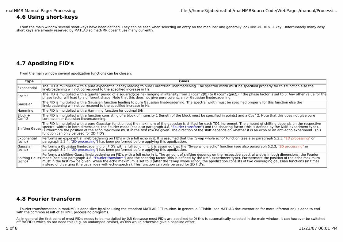
From the main window several apodization functions can be chosen:
Type Gives
Exponential The FID is multiplied with a pure exponential decay leading to pure Lorentzian linebroadening. The spectral width must be specified properly for this function else thelinebroadening will not correspond to the specified increase in Hz.
Cos^2 The FID is multiplied with a quarter period of a squared(cosine) ranging in intensity from 1 (cos^2(0)) to 0 (cos^2(pi/2)) if the phase factor is set to 0. Any other value for thephase factor will lead to a different shape. Note that this does not give pure Lorentzian or Gaussian linebroadening.
Gaussian The FID is multiplied with a Gaussian function leading to pure Gaussian linebroadening. The spectral width must be specified properly for this function else thelinebroadening will not correspond to the specified increase in Hz.
Hamming The FID is multiplied with a Hamming function for optimal S/N.
Block + Cos^2
The FID is multiplied with a function consisting of a block of intensity 1 (length of the block must be specified in points) and a Cos^2. Note that this does not give pureLorentzian or Gaussian linebroadening.
Shifting Gauss
The FID is multiplied with a pure Gaussian function but the maximum of the gaussian is shifted for each TD1 increment. The amount of shifting depends on the respectivespectral widths in both dimensions, the Fourier mode (see also paragraph 4.8, "Fourier transform") and the shearing factor (this is defined by the NMR experiment type).Furthermore the position of the echo maximum must in the first row be given. The direction of the shift depends on whether it is an echo or an anti-echo experiment. Thisfunction can only be used for 2D FID's.
Exponential (echo)
Performs an exponential linebroadening on FID's with a full echo in it. It is assumed that the "Swap whole echo" function (see also paragraph 5.2.3, "1D processing" or paragraph 5.2.4, "2D processing") has been performed before applying this apodization.
Gaussian (echo)
Performs a Gaussian linebroadening on FID's with a full echo in it. It is assumed that the "Swap whole echo" function (see also paragraph 5.2.3, "1D processing" or paragraph 5.2.4, "2D processing") has been performed before applying this apodization.
Shifting Gauss (echo)
Performs a shifting-Gauss linebroadening on FID's with a full echo in it. The amount of shifting depends on the respective spectral widths in both dimensions, the Fouriermode (see also paragraph 4.8, "Fourier transform") and the shearing factor (this is defined by the NMR experiment type). Furthermore the position of the echo maximummust in the first row be given. When the echo maximum is set to 0 (after the "swap whole echo") the apodization consists of two converging gaussian functions (in time)instead of diverging (the usual idea with echo-spectra). This function can only be used for 2D FID's.
4.8 Fourier transform
Fourier transformation in matNMR is done slice-by-slice using the standard MATLAB FFT routine. In general a FFTshift (see MATLAB documentation for more information) is done to endwith the common result of all NMR processing programs.
As in general the first point of most FID's needs to be multiplied by 0.5 (because most FID's are apodized to 0) this is automatically selected in the main window. It can however be switchedoff for FID's which do not need this (e.g. an undamped cosine), as this would otherwise give a baseline offset.
matNMR Manual Page: Processing file:///home3/jabe/matlab/matNMRSourceCode/WebPages/manual/Processi...
6 of 8 11/23/07 06:01 PM
The inverse FT can also be performed, but has to be accessed from the "Additional Features" item in either the "1D Processing" or "2D Processing" menus in the menubar.
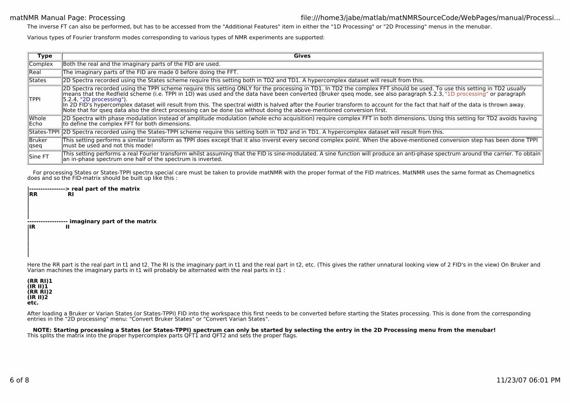
Various types of Fourier transform modes corresponding to various types of NMR experiments are supported:
Type Gives
Complex Both the real and the imaginary parts of the FID are used.
Real The imaginary parts of the FID are made 0 before doing the FFT.
States 2D Spectra recorded using the States scheme require this setting both in TD2 and TD1. A hypercomplex dataset will result from this.
TPPI
2D Spectra recorded using the TPPI scheme require this setting ONLY for the processing in TD1. In TD2 the complex FFT should be used. To use this setting in TD2 usuallymeans that the Redfield scheme (i.e. TPPI in 1D) was used and the data have been converted (Bruker qseq mode, see also paragraph 5.2.3, "1D processing" or paragraph 5.2.4, "2D processing"). In 2D FID's hypercomplex dataset will result from this. The spectral width is halved after the Fourier transform to account for the fact that half of the data is thrown away. Note that for qseq data also the direct processing can be done (so without doing the above-mentioned conversion first.
Whole Echo
2D Spectra with phase modulation instead of amplitude modulation (whole echo acquisition) require complex FFT in both dimensions. Using this setting for TD2 avoids havingto define the complex FFT for both dimensions.
States-TPPI 2D Spectra recorded using the States-TPPI scheme require this setting both in TD2 and in TD1. A hypercomplex dataset will result from this.
Bruker qseq
This setting performs a similar transform as TPPI does except that it also inverst every second complex point. When the above-mentioned conversion step has been done TPPImust be used and not this mode!
Sine FT This setting performs a real Fourier transform whilst assuming that the FID is sine-modulated. A sine function will produce an anti-phase spectrum around the carrier. To obtainan in-phase spectrum one half of the spectrum is inverted.
For processing States or States-TPPI spectra special care must be taken to provide matNMR with the proper format of the FID matrices. MatNMR uses the same format as Chemagneticsdoes and so the FID-matrix should be built up like this :
|----------------> real part of the matrix|RR RI||||------------------ imaginary part of the matrix|IR II|||||
Here the RR part is the real part in t1 and t2. The RI is the imaginary part in t1 and the real part in t2, etc. (This gives the rather unnatural looking view of 2 FID's in the view) On Bruker andVarian machines the imaginary parts in t1 will probably be alternated with the real parts in t1 :
(RR RI)1(IR II)1(RR RI)2(IR II)2etc.
After loading a Bruker or Varian States (or States-TPPI) FID into the workspace this first needs to be converted before starting the States processing. This is done from the correspondingentries in the "2D processing" menu: "Convert Bruker States" or "Convert Varian States".
NOTE: Starting processing a States (or States-TPPI) spectrum can only be started by selecting the entry in the 2D Processing menu from the menubar!This splits the matrix into the proper hypercomplex parts QFT1 and QFT2 and sets the proper flags.
matNMR Manual Page: Processing file:///home3/jabe/matlab/matNMRSourceCode/WebPages/manual/Processi...
7 of 8 11/23/07 06:01 PM
4.9 Phasing spectra
Phase correction of spectra is done using the phase menu (see also paragraph 5.1, "General appearance"). There are several ways to set the zeroth-order, first-order and second-orderphase correction: There is a slider button, an edit button for writing the value in directly and there are step-wise incremental buttons (small and big steps). To set the first-order correction areference position must be specified. This can be done by clicking on the "Reference Ph1" button. A cross-hair will appear to aid finding the proper peak position. Clicking the left mousebutton defines the position. The "zero phases" button will set the phasing values to zero again.
Note that to set the second-order phase correction one needs to push the check button in order to open an extra panel (since it is not commonly used). The reference for the 2nd orderphase correction is always in the center of the spectrum since it is used to even out the effects of sharp cut-offs in modern audio filters; these effects are symmetrical around the center ofthe spectrum.
While phase correcting a 2D spectrum it is often necessary to watch different slices to see whether the new phase values are any good. Switching to a new row or column (while notswitching dimension!) will show this row/column with the phase values shown in the phase menu on screen. Only when switching dimension will the phase values be reset again.Alternatively to switching between slices one may use the "2D tool", which allows watching two additional slices/columns from which the quality of the phase correction may be estimated.The additional plots are updated with each change of the phase.After having found a good phase correction for a 2D be sure to press the "Set Phase 2D" button to impose the new phase correction on the entire 2D matrix!
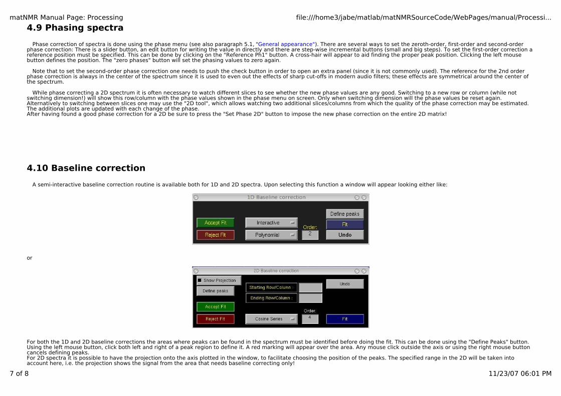
4.10 Baseline correction
A semi-interactive baseline correction routine is available both for 1D and 2D spectra. Upon selecting this function a window will appear looking either like:
or
For both the 1D and 2D baseline corrections the areas where peaks can be found in the spectrum must be identified before doing the fit. This can be done using the "Define Peaks" button.Using the left mouse button, click both left and right of a peak region to define it. A red marking will appear over the area. Any mouse click outside the axis or using the right mouse buttoncancels defining peaks.For 2D spectra it is possible to have the projection onto the axis plotted in the window, to facilitate choosing the position of the peaks. The specified range in the 2D will be taken intoaccount here, i.e. the projection shows the signal from the area that needs baseline correcting only!

matNMR Manual Page: Processing file:///home3/jabe/matlab/matNMRSourceCode/WebPages/manual/Processi...
8 of 8 11/23/07 06:01 PM
Next, the type of function that needs to be used for fitting the baseline must be specified. Currently one can choose from either a cosine series, a polynomial or a Bernstein polynomial.These are defined as:
Polynomial of order 6: 'A + B*x + C*x.^2 + D*x.^3 + E*x.^4 + F*x.^5'Cosine series of order 6: 'A + B*cos(x) + C*cos(2*x) + D*cos(3*x) + E*cos(4*x) + F*cos(5*x)'Bernstein of order 6: 'A*(1-x).^5 + B*(x).*((1-x).^4) + C*(x.^2).*((1-x).^3) + D*(x.^3).*((1-x).^2) + E*(x.^4).*(1-x) + F*(x.^5)'Sine: 'A + B * sin(C*x + D)'Exponential: 'A + B * exp(C*x)'
where A-F are the coefficients to be fitted to the baseline and x the coordinate along the spectral axis. After choosing the order to which the fit should go, and pressing "Fit" the fit isperformed. Any order of fit is allowed but beware that a fit will become very bad when the order is too high.
The resulting 1D spectrum or row/column from the 2D will be shown in the view. For 1D baseline correction also the fitted baseline is shown in blue as a visual aid. To see the result of thebaseline correction for the whole 2D just step through the rows/columns.
Should the baseline be satisfactory then the "Accept Fit" button must be pressed and the fit is made final. If not, either press "Undo" to obtain the original spectrum back or "Reject Fit" toreject the fit and stop the baseline correction routine while retaining the original spectrum.
matNMR Manual Page: MainWindow file:///home3/jabe/matlab/matNMRSourceCode/WebPages/manual/MainWi...
1 of 42 11/23/07 06:02 PM
Chapter 5 - The main windowThe main window is started using the nmr.m script, i.e. type 'nmr' at the Matlab prompt to start it. All processing is done from this window and all other functionality implemented in
matNMR can be accessed from the menubar or the Uicontrols.
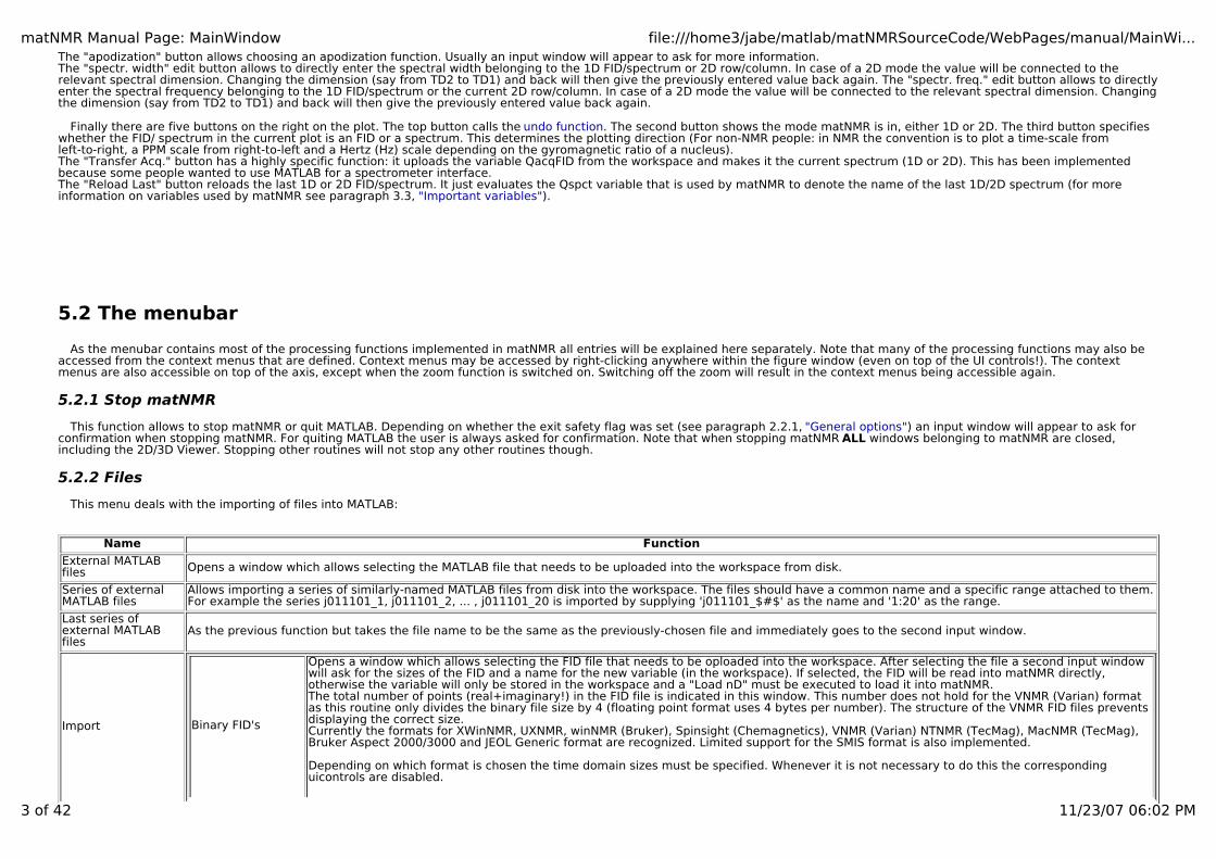
5.1 General Appearance
The general appearance of the matNMR main window is shown in the figure below:

matNMR Manual Page: MainWindow file:///home3/jabe/matlab/matNMRSourceCode/WebPages/manual/MainWi...
2 of 42 11/23/07 06:02 PM
There are five boxes shaded with a background box around it. Going from top-left to bottom-right they contain1- a stop-button, a direct-printing button (prints to the default printer as defined in the $matlabroot/toolbox/local/printopt.m file) and some buttons to open the various menus2- some often-used buttons for working with 1D spectra. More functions can be found in the menubar.3- the phasing menu. (see also paragraph 4.9, "Phasing spectra")4- some buttons for zooming in discrete steps or continously (zoom button). Furthermore there is the "reset figure" button which resets the current view (leaving nothing but the current 1Dspectrum Qspc2 in the view!) and the "get position" button allows to scan the lines in the plot using the mouse pointer. Upon pressing the left mouse button a crosshair will appear andsome buttons that show the coordinate and the intensity of the current trace. When more than one lines are in the plot a popup button will appear to choose which line the routine shouldfollow.5- some often-used buttons for working with 2D spectra. More functions can be found in the menubar.
Then there are some buttons just above the box with zoom functions.The "display mode" is for defining whether to show the real, imaginary or absolute value of a FID/ spectrum. Note that this is only a matter of displaying. MatNMR always works with complexvalues.The "fourier mode" defines what type of FFT is performed when the FFT-button is pressed (see also paragraph 4.8, "Fourier transform").
matNMR Manual Page: MainWindow file:///home3/jabe/matlab/matNMRSourceCode/WebPages/manual/MainWi...
3 of 42 11/23/07 06:02 PM
The "apodization" button allows choosing an apodization function. Usually an input window will appear to ask for more information.The "spectr. width" edit button allows to directly enter the spectral width belonging to the 1D FID/spectrum or 2D row/column. In case of a 2D mode the value will be connected to therelevant spectral dimension. Changing the dimension (say from TD2 to TD1) and back will then give the previously entered value back again. The "spectr. freq." edit button allows to directlyenter the spectral frequency belonging to the 1D FID/spectrum or the current 2D row/column. In case of a 2D mode the value will be connected to the relevant spectral dimension. Changingthe dimension (say from TD2 to TD1) and back will then give the previously entered value back again.
Finally there are five buttons on the right on the plot. The top button calls the undo function. The second button shows the mode matNMR is in, either 1D or 2D. The third button specifieswhether the FID/ spectrum in the current plot is an FID or a spectrum. This determines the plotting direction (For non-NMR people: in NMR the convention is to plot a time-scale fromleft-to-right, a PPM scale from right-to-left and a Hertz (Hz) scale depending on the gyromagnetic ratio of a nucleus).The "Transfer Acq." button has a highly specific function: it uploads the variable QacqFID from the workspace and makes it the current spectrum (1D or 2D). This has been implementedbecause some people wanted to use MATLAB for a spectrometer interface.The "Reload Last" button reloads the last 1D or 2D FID/spectrum. It just evaluates the Qspct variable that is used by matNMR to denote the name of the last 1D/2D spectrum (for moreinformation on variables used by matNMR see paragraph 3.3, "Important variables").
5.2 The menubar
As the menubar contains most of the processing functions implemented in matNMR all entries will be explained here separately. Note that many of the processing functions may also beaccessed from the context menus that are defined. Context menus may be accessed by right-clicking anywhere within the figure window (even on top of the UI controls!). The contextmenus are also accessible on top of the axis, except when the zoom function is switched on. Switching off the zoom will result in the context menus being accessible again.
5.2.1 Stop matNMR
This function allows to stop matNMR or quit MATLAB. Depending on whether the exit safety flag was set (see paragraph 2.2.1, "General options") an input window will appear to ask forconfirmation when stopping matNMR. For quiting MATLAB the user is always asked for confirmation. Note that when stopping matNMR ALL windows belonging to matNMR are closed,including the 2D/3D Viewer. Stopping other routines will not stop any other routines though.
5.2.2 Files
This menu deals with the importing of files into MATLAB:
Name Function
External MATLAB files Opens a window which allows selecting the MATLAB file that needs to be uploaded into the workspace from disk.
Series of external MATLAB files
Allows importing a series of similarly-named MATLAB files from disk into the workspace. The files should have a common name and a specific range attached to them.For example the series j011101_1, j011101_2, ... , j011101_20 is imported by supplying 'j011101_$#$' as the name and '1:20' as the range.
Last series of external MATLAB files
As the previous function but takes the file name to be the same as the previously-chosen file and immediately goes to the second input window.
Import Binary FID's
Opens a window which allows selecting the FID file that needs to be oploaded into the workspace. After selecting the file a second input windowwill ask for the sizes of the FID and a name for the new variable (in the workspace). If selected, the FID will be read into matNMR directly,otherwise the variable will only be stored in the workspace and a "Load nD" must be executed to load it into matNMR.The total number of points (real+imaginary!) in the FID file is indicated in this window. This number does not hold for the VNMR (Varian) formatas this routine only divides the binary file size by 4 (floating point format uses 4 bytes per number). The structure of the VNMR FID files preventsdisplaying the correct size.Currently the formats for XWinNMR, UXNMR, winNMR (Bruker), Spinsight (Chemagnetics), VNMR (Varian) NTNMR (TecMag), MacNMR (TecMag),Bruker Aspect 2000/3000 and JEOL Generic format are recognized. Limited support for the SMIS format is also implemented.
Depending on which format is chosen the time domain sizes must be specified. Whenever it is not necessary to do this the correspondinguicontrols are disabled.
matNMR Manual Page: MainWindow file:///home3/jabe/matlab/matNMRSourceCode/WebPages/manual/MainWi...
4 of 42 11/23/07 06:02 PM
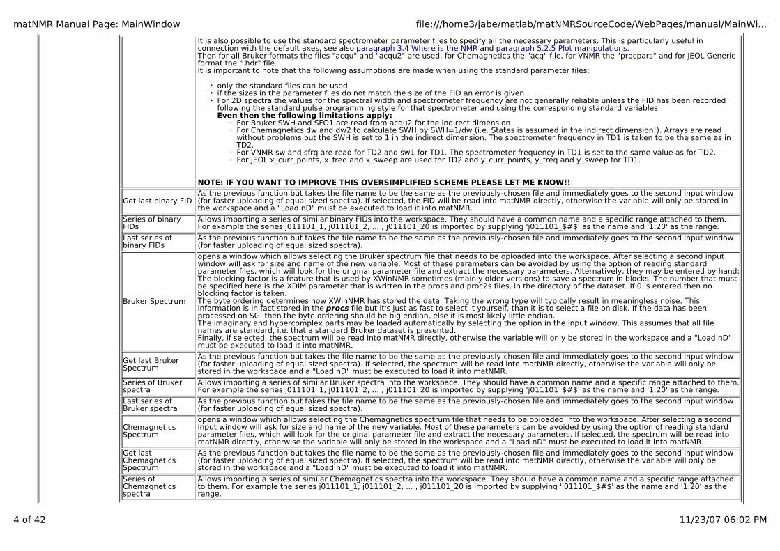
It is also possible to use the standard spectrometer parameter files to specify all the necessary parameters. This is particularly useful inconnection with the default axes, see also paragraph 3.4 Where is the NMR and paragraph 5.2.5 Plot manipulations.Then for all Bruker formats the files "acqu" and "acqu2" are used, for Chemagnetics the "acq" file, for VNMR the "procpars" and for JEOL Genericformat the ".hdr" file. It is important to note that the following assumptions are made when using the standard parameter files:
only the standard files can be usedif the sizes in the parameter files do not match the size of the FID an error is givenFor 2D spectra the values for the spectral width and spectrometer frequency are not generally reliable unless the FID has been recordedfollowing the standard pulse programming style for that spectrometer and using the corresponding standard variables. Even then the following limitations apply:
For Bruker SWH and SFO1 are read from acqu2 for the indirect dimensionFor Chemagnetics dw and dw2 to calculate SWH by SWH=1/dw (i.e. States is assumed in the indirect dimension!). Arrays are readwithout problems but the SWH is set to 1 in the indirect dimension. The spectrometer frequency in TD1 is taken to be the same as inTD2.For VNMR sw and sfrq are read for TD2 and sw1 for TD1. The spectrometer frequency in TD1 is set to the same value as for TD2.For JEOL x_curr_points, x_freq and x_sweep are used for TD2 and y_curr_points, y_freq and y_sweep for TD1.
NOTE: IF YOU WANT TO IMPROVE THIS OVERSIMPLIFIED SCHEME PLEASE LET ME KNOW!!
Get last binary FIDAs the previous function but takes the file name to be the same as the previously-chosen file and immediately goes to the second input window(for faster uploading of equal sized spectra). If selected, the FID will be read into matNMR directly, otherwise the variable will only be stored inthe workspace and a "Load nD" must be executed to load it into matNMR.
Series of binary FIDs
Allows importing a series of similar binary FIDs into the workspace. They should have a common name and a specific range attached to them.For example the series j011101_1, j011101_2, ... , j011101_20 is imported by supplying 'j011101_$#$' as the name and '1:20' as the range.
Last series of binary FIDs
As the previous function but takes the file name to be the same as the previously-chosen file and immediately goes to the second input window(for faster uploading of equal sized spectra).
Bruker Spectrum
opens a window which allows selecting the Bruker spectrum file that needs to be oploaded into the workspace. After selecting a second inputwindow will ask for size and name of the new variable. Most of these parameters can be avoided by using the option of reading standardparameter files, which will look for the original parameter file and extract the necessary parameters. Alternatively, they may be entered by hand:The blocking factor is a feature that is used by XWinNMR sometimes (mainly older versions) to save a spectrum in blocks. The number that mustbe specified here is the XDIM parameter that is written in the procs and proc2s files, in the directory of the dataset. If 0 is entered then noblocking factor is taken.The byte ordering determines how XWinNMR has stored the data. Taking the wrong type will typically result in meaningless noise. Thisinformation is in fact stored in the procs file but it's just as fast to select it yourself, than it is to select a file on disk. If the data has beenprocessed on SGI then the byte ordering should be big endian, else it is most likely little endian.The imaginary and hypercomplex parts may be loaded automatically by selecting the option in the input window. This assumes that all filenames are standard, i.e. that a standard Bruker dataset is presented.Finally, if selected, the spectrum will be read into matNMR directly, otherwise the variable will only be stored in the workspace and a "Load nD"must be executed to load it into matNMR.
Get last Bruker Spectrum
As the previous function but takes the file name to be the same as the previously-chosen file and immediately goes to the second input window(for faster uploading of equal sized spectra). If selected, the spectrum will be read into matNMR directly, otherwise the variable will only bestored in the workspace and a "Load nD" must be executed to load it into matNMR.
Series of Bruker spectra
Allows importing a series of similar Bruker spectra into the workspace. They should have a common name and a specific range attached to them.For example the series j011101_1, j011101_2, ... , j011101_20 is imported by supplying 'j011101_$#$' as the name and '1:20' as the range.
Last series of Bruker spectra
As the previous function but takes the file name to be the same as the previously-chosen file and immediately goes to the second input window(for faster uploading of equal sized spectra).
Chemagnetics Spectrum
opens a window which allows selecting the Chemagnetics spectrum file that needs to be oploaded into the workspace. After selecting a secondinput window will ask for size and name of the new variable. Most of these parameters can be avoided by using the option of reading standardparameter files, which will look for the original parameter file and extract the necessary parameters. If selected, the spectrum will be read intomatNMR directly, otherwise the variable will only be stored in the workspace and a "Load nD" must be executed to load it into matNMR.
Get last Chemagnetics Spectrum
As the previous function but takes the file name to be the same as the previously-chosen file and immediately goes to the second input window(for faster uploading of equal sized spectra). If selected, the spectrum will be read into matNMR directly, otherwise the variable will only bestored in the workspace and a "Load nD" must be executed to load it into matNMR.
Series of Chemagnetics spectra
Allows importing a series of similar Chemagnetics spectra into the workspace. They should have a common name and a specific range attachedto them. For example the series j011101_1, j011101_2, ... , j011101_20 is imported by supplying 'j011101_$#$' as the name and '1:20' as therange.

matNMR Manual Page: MainWindow file:///home3/jabe/matlab/matNMRSourceCode/WebPages/manual/MainWi...
5 of 42 11/23/07 06:02 PM
Last series of Chemagnetics spectra
As the previous function but takes the file name to be the same as the previously-chosen file and immediately goes to the second input window(for faster uploading of equal sized spectra).
SIMPSON ASCIIopens a window which allows selecting the SIMPSON ASCII file that needs to be oploaded into the workspace. After selecting a second inputwindow will ask for the name of the new variable. If selected, the spectrum will be read into matNMR directly, otherwise the variable will only bestored in the workspace and a "Load nD" must be executed to load it into matNMR.
Get last SIMPSON ASCII
As the previous function but takes the file name to be the same as the previously-chosen file and immediately goes to the second input window(for faster uploading of similarly named spectra). If selected, the spectrum will be read into matNMR directly, otherwise the variable will only bestored in the workspace and a "Load nD" must be executed to load it into matNMR.
Series of SIMPSON ASCII
Allows importing a series of similarly-named SIMPSON ASCII files into the workspace. They should have a common name and a specific rangeattached to them. For example the series j011101_1, j011101_2, ... , j011101_20 is imported by supplying 'j011101_$#$' as the name and '1:20'as the range.
Last series of SIMPSON ASCII
As the previous function but takes the file name to be the same as the previously-chosen file and immediately goes to the second input window(for faster uploading of equal sized spectra).
Export Save as SIMPSON ASCII opens a window which allows selecting a file thatis used to store the current 1D or 2D on disk in SIMPSON ASCII format.
Series Trickery
These functions allow all sorts of actions to be done on a series of variables in the workspace, which have common names and a specific range attached to them. Forexample the series j011101_1, j011101_2, ... , j011101_20 can be addressed by supplying 'j011101_$#$' as the name and '1:20' as the range. The following functionshave been defined currently.Add series of variables Allows adding a series of variables.
Concatenate series of variables Allows concatenating a series of variables in the workspace, which have a common name and a specific range attached to them.
Normalize series of variables
Allows normalizing a series of variables in the workspace, which have a common name and a specific range attached to them, to eitherthe same maximum or the same integral.
Change directory Sets the current directory path
Set search profile Sets the search profile for binary FID's / Bruker spectra / SIMPSON ASCII files
Edit MATLAB path Starts the MATLAB search path editor
Edit Workspace Starts the MATLAB workspace editor
Editor/Debugger Starts the MATLAB m-file editor/debugger
5.2.3 1D Processing
This menu deals with everything concerning working with 1D spectra:
Name Function
Load 1D Gets a new 1D spectrum. An axis vector may be specified and also whether the variable is an FID or a spectrum (see also button information in paragraph 5.1, "General appearance").
Add Spectrum to Workspace
Saves the current 1D spectrum to the workspace. Depending on whether the history and/or axis vector must be included a matNMR structure will be created (also seeparagraph 3.5, "matNMR format for spectra").
Save Spectrum to Disk
As the previous function but saves the variable to disk. In case more than one variable names are given in the input window it will save the variables without doinganything with the current 1D spectrum!
Dual display
Adds an additional line to the view. If no axis vector is specified then the current axis vector Qtempvec1d will be used. Note that the new spectrum must have the samesize then. If a spectrum of different size is given then an axis vector MUST be specified. Spectra that are added to the view using "dual plot" do not influence anyprocessing steps. Every time the plot is refreshed by matNMR (or by applying the "reset figure" button, see paragraph 5.1, "General appearance") they will be removed.
Various plot types are supported by the dual plot routine: normal plots, horizontal stack plots, vertical stack plots, 1D bar plots and errorbar plots. This will affect theinput window that will pop up when selecting this function.
Convert Bruker qseq
The Bruker qseq acquisition mode is basically TPPI in 1D. This in principle should be a real vector but when loading a binary the FID is in fact complex. This functionconverts the FID into a real vector with all real and imaginary points concatenated and every second complex point inverted:R I R I R I R I R I R I R I...
matNMR Manual Page: MainWindow file:///home3/jabe/matlab/matNMRSourceCode/WebPages/manual/MainWi...
6 of 42 11/23/07 06:02 PM
This function does not need to be used as the qseq mode for FT allows direct processing but is recommended. Direct processing in principal does not allow furthermanipulation (e.g. apodization is ever so slightly wrong when applying it to the complex vector).
Standard Processing
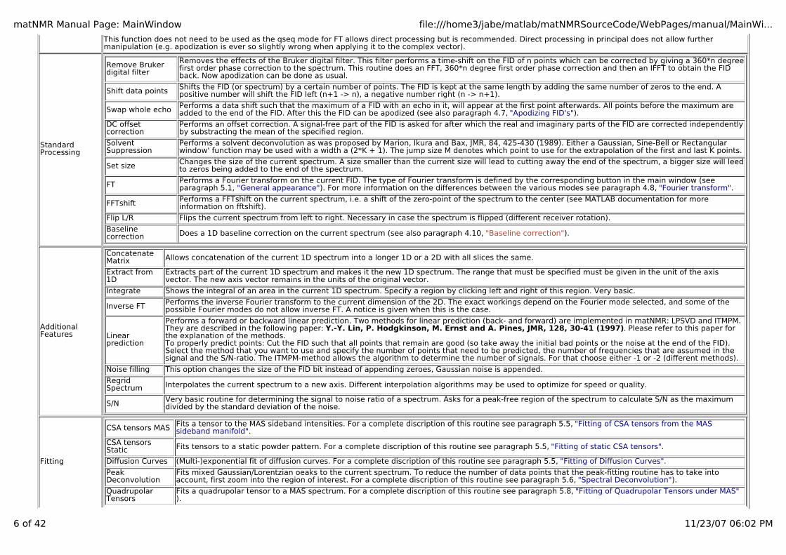
Remove Bruker digital filter
Removes the effects of the Bruker digital filter. This filter performs a time-shift on the FID of n points which can be corrected by giving a 360*n degreefirst order phase correction to the spectrum. This routine does an FFT, 360*n degree first order phase correction and then an IFFT to obtain the FIDback. Now apodization can be done as usual.
Shift data points Shifts the FID (or spectrum) by a certain number of points. The FID is kept at the same length by adding the same number of zeros to the end. Apositive number will shift the FID left (n+1 -> n), a negative number right (n -> n+1).
Swap whole echo Performs a data shift such that the maximum of a FID with an echo in it, will appear at the first point afterwards. All points before the maximum areadded to the end of the FID. After this the FID can be apodized (see also paragraph 4.7, "Apodizing FID's").
DC offset correction
Performs an offset correction. A signal-free part of the FID is asked for after which the real and imaginary parts of the FID are corrected independentlyby substracting the mean of the specified region.
Solvent Suppression
Performs a solvent deconvolution as was proposed by Marion, Ikura and Bax, JMR, 84, 425-430 (1989). Either a Gaussian, Sine-Bell or Rectangularwindow' function may be used with a width a (2*K + 1). The jump size M denotes which point to use for the extrapolation of the first and last K points.
Set size Changes the size of the current spectrum. A size smaller than the current size will lead to cutting away the end of the spectrum, a bigger size will leedto zeros being added to the end of the spectrum.
FT Performs a Fourier transform on the current FID. The type of Fourier transform is defined by the corresponding button in the main window (seeparagraph 5.1, "General appearance"). For more information on the differences between the various modes see paragraph 4.8, "Fourier transform".
FFTshift Performs a FFTshift on the current spectrum, i.e. a shift of the zero-point of the spectrum to the center (see MATLAB documentation for moreinformation on fftshift).
Flip L/R Flips the current spectrum from left to right. Necessary in case the spectrum is flipped (different receiver rotation).
Baseline correction Does a 1D baseline correction on the current spectrum (see also paragraph 4.10, "Baseline correction").
Additional Features
Concatenate Matrix Allows concatenation of the current 1D spectrum into a longer 1D or a 2D with all slices the same.
Extract from 1D
Extracts part of the current 1D spectrum and makes it the new 1D spectrum. The range that must be specified must be given in the unit of the axisvector. The new axis vector remains in the units of the original vector.
Integrate Shows the integral of an area in the current 1D spectrum. Specify a region by clicking left and right of this region. Very basic.
Inverse FT Performs the inverse Fourier transform to the current dimension of the 2D. The exact workings depend on the Fourier mode selected, and some of thepossible Fourier modes do not allow inverse FT. A notice is given when this is the case.
Linear prediction
Performs a forward or backward linear prediction. Two methods for linear prediction (back- and forward) are implemented in matNMR: LPSVD and ITMPM.They are described in the following paper: Y.-Y. Lin, P. Hodgkinson, M. Ernst and A. Pines, JMR, 128, 30-41 (1997). Please refer to this paper for the explanation of the methods.To properly predict points: Cut the FID such that all points that remain are good (so take away the initial bad points or the noise at the end of the FID).Select the method that you want to use and specify the number of points that need to be predicted, the number of frequencies that are assumed in thesignal and the S/N-ratio. The ITMPM-method allows the algorithm to determine the number of signals. For that choose either -1 or -2 (different methods).
Noise filling This option changes the size of the FID bit instead of appending zeroes, Gaussian noise is appended.
Regrid Spectrum Interpolates the current spectrum to a new axis. Different interpolation algorithms may be used to optimize for speed or quality.
S/N Very basic routine for determining the signal to noise ratio of a spectrum. Asks for a peak-free region of the spectrum to calculate S/N as the maximumdivided by the standard deviation of the noise.
Fitting
CSA tensors MAS Fits a tensor to the MAS sideband intensities. For a complete discription of this routine see paragraph 5.5, "Fitting of CSA tensors from the MAS sideband manifold".
CSA tensors Static Fits tensors to a static powder pattern. For a complete discription of this routine see paragraph 5.5, "Fitting of static CSA tensors".
Diffusion Curves (Multi-)exponential fit of diffusion curves. For a complete discription of this routine see paragraph 5.5, "Fitting of Diffusion Curves".
Peak Deconvolution
Fits mixed Gaussian/Lorentzian oeaks to the current spectrum. To reduce the number of data points that the peak-fitting routine has to take intoaccount, first zoom into the region of interest. For a complete discription of this routine see paragraph 5.6, "Spectral Deconvolution").
Quadrupolar Tensors
Fits a quadrupolar tensor to a MAS spectrum. For a complete discription of this routine see paragraph 5.8, "Fitting of Quadrupolar Tensors under MAS").
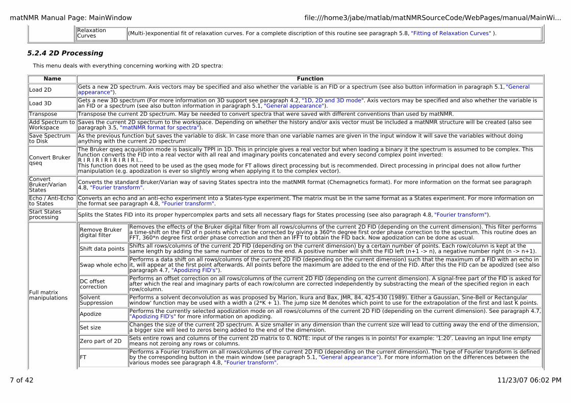
matNMR Manual Page: MainWindow file:///home3/jabe/matlab/matNMRSourceCode/WebPages/manual/MainWi...
7 of 42 11/23/07 06:02 PM
Relaxation Curves (Multi-)exponential fit of relaxation curves. For a complete discription of this routine see paragraph 5.8, "Fitting of Relaxation Curves" ).
5.2.4 2D Processing
This menu deals with everything concerning working with 2D spectra:
Name Function
Load 2D Gets a new 2D spectrum. Axis vectors may be specified and also whether the variable is an FID or a spectrum (see also button information in paragraph 5.1, "General appearance").
Load 3D Gets a new 3D spectrum (For more information on 3D support see paragraph 4.2, "1D, 2D and 3D mode". Axis vectors may be specified and also whether the variable isan FID or a spectrum (see also button information in paragraph 5.1, "General appearance").
Transpose Transpose the current 2D spectrum. May be needed to convert spectra that were saved with different conventions than used by matNMR.
Add Spectrum to Workspace
Saves the current 2D spectrum to the workspace. Depending on whether the history and/or axis vector must be included a matNMR structure will be created (also seeparagraph 3.5, "matNMR format for spectra").
Save Spectrum to Disk
As the previous function but saves the variable to disk. In case more than one variable names are given in the input window it will save the variables without doinganything with the current 2D spectrum!
Convert Bruker qseq
The Bruker qseq acquisition mode is basically TPPI in 1D. This in principle gives a real vector but when loading a binary it the spectrum is assumed to be complex. Thisfunction converts the FID into a real vector with all real and imaginary points concatenated and every second complex point inverted:R I R I R I R I R I R I R I...This function does not need to be used as the qseq mode for FT allows direct processing but is recommended. Direct processing in principal does not allow furthermanipulation (e.g. apodization is ever so slightly wrong when applying it to the complex vector).
Convert Bruker/Varian States
Converts the standard Bruker/Varian way of saving States spectra into the matNMR format (Chemagnetics format). For more information on the format see paragraph4.8, "Fourier transform".
Echo / Anti-Echo to States
Converts an echo and an anti-echo experiment into a States-type experiment. The matrix must be in the same format as a States experiment. For more information onthe format see paragraph 4.8, "Fourier transform".
Start States processing Splits the States FID into its proper hypercomplex parts and sets all necessary flags for States processing (see also paragraph 4.8, "Fourier transform").
Full matrix manipulations
Remove Bruker digital filter
Removes the effects of the Bruker digital filter from all rows/columns of the current 2D FID (depending on the current dimension). This filter performsa time-shift on the FID of n points which can be corrected by giving a 360*n degree first order phase correction to the spectrum. This routine does anFFT, 360*n degree first order phase correction and then an IFFT to obtain the FID back. Now apodization can be done as usual.
Shift data points Shifts all rows/columns of the current 2D FID (depending on the current dimension) by a certain number of points. Each row/column is kept at thesame length by adding the same number of zeros to the end. A positive number will shift the FID left (n+1 -> n), a negative number right (n -> n+1).
Swap whole echoPerforms a data shift on all rows/columns of the current 2D FID (depending on the current dimension) such that the maximum of a FID with an echo init, will appear at the first point afterwards. All points before the maximum are added to the end of the FID. After this the FID can be apodized (see alsoparagraph 4.7, "Apodizing FID's").
DC offset correction
Performs an offset correction on all rows/columns of the current 2D FID (depending on the current dimension). A signal-free part of the FID is asked forafter which the real and imaginary parts of each row/column are corrected independently by substracting the mean of the specified region in eachrow/column.
Solvent Suppression
Performs a solvent deconvolution as was proposed by Marion, Ikura and Bax, JMR, 84, 425-430 (1989). Either a Gaussian, Sine-Bell or Rectangularwindow' function may be used with a width a (2*K + 1). The jump size M denotes which point to use for the extrapolation of the first and last K points.
Apodize Performs the currently selected apodization mode on all rows/columns of the current 2D FID (depending on the current dimension). See paragraph 4.7,"Apodizing FID's" for more information on apodizing.
Set size Changes the size of the current 2D spectrum. A size smaller in any dimension than the current size will lead to cutting away the end of the dimension,a bigger size will leed to zeros being added to the end of the dimension.
Zero part of 2D Sets entire rows and columns of the current 2D matrix to 0. NOTE: input of the ranges is in points! For example: '1:20'. Leaving an input line emptymeans not zeroing any rows or columns.
FTPerforms a Fourier transform on all rows/columns of the current 2D FID (depending on the current dimension). The type of Fourier transform is definedby the corresponding button in the main window (see paragraph 5.1, "General appearance"). For more information on the differences between thevarious modes see paragraph 4.8, "Fourier transform".

matNMR Manual Page: MainWindow file:///home3/jabe/matlab/matNMRSourceCode/WebPages/manual/MainWi...
8 of 42 11/23/07 06:02 PM
FFTshift Performs a FFTshift on all rows/columns of the current 2D FID (depending on the current dimension), i.e. a shift of the zero-point of the row/columns tothe center (see MATLAB documentation for more information on fftshift).
Flip L/R Flips all rows/columns of the current 2D spectrum (depending on the current dimension) from left to right. Necessary in case the spectrum is flipped(different receiver rotation).
Set Phase Performs the currently selected phase correction on all rows/columns of the current 2D FID (depending on the current dimension). See paragraph 4.9,"Phasing spectra" for more information on phase correction.
Baseline correction Does a 2D baseline correction on the current spectrum (see also paragraph 4.10, "Baseline correction" ).
Single Slice Manipulations
This submenu allows the manipulations of the current row/column of the current 2D, without the rest of the matrix being affected. Look at the entries for the regularfunctions to see what they do.
Additional Features
Concatenate Matrix Allows concatenation of the current 2D spectrum into a bigger 2D spectrum. Concatenation can be done in both directions.
Extract from 2D Extracts part of the current 2D spectrum and makes it the new 2D spectrum. The range that must be specified must be given in the unit of the axisvector. The new axis vectors remain in the units of the original vectors.
Integrate Fixed range
Calculates the integral of a part of a spectrum by selecting a region of the current 2D spectrum (in units of the axis vectors) and adding all intensities.The output is a variable in the workspace with the intensities, the axis in the current dimension and the position of the maximum signal in units of itsoriginal axis.
Integrate around Max
Shows the integral of an area in the current 1D spectrum. This routine searches in each slice in the 2D for the maximum signal in a user-specifiedrange and integrates with a user-specified range around that maximum. This allows integration of peaks with variable positions and possiblyoverlapping other peaks. The output is a variable in the workspace with the intensities, the axis in the current dimension and the position of themaximum signal in units of its original axis.
Inverse FT Performs the inverse Fourier transform to the current dimension of the 2D. The exact workings depend on the Fourier mode selected, and some of thepossible Fourier modes do not allow inverse FT. A notice is given when this is the case.
Linear prediction
Performs a forward or backward linear prediction on all rows/columns of the current 2D spectrum (depending on the current dimension). Two methodsfor linear prediction (back- and forward) are implemented in matNMR: LPSVD and ITMPM. They are described in the following paper: Y.-Y. Lin, P. Hodgkinson, M. Ernst and A. Pines, JMR, 128, 30-41 (1997). Please refer to this paper for the explanation of the methods.To properly predict points: Cut the FID such that all points that remain are good (so take away the initial bad points or the noise at the end of the FID).Select the method that you want to use and specify the number of points that need to be predicted, the number of frequencies that are assumed in thesignal and the S/N-ratio. The ITMPM-method allows the algorithm to determine the number of signals. For that choose either -1 or -2 (differentmethods).
Noise filling This option changes the size of the FID bit instead of appending zeroes, Gaussian noise is appended.
Regrid Spectrum Interpolates the current spectrum to a new axis. Different interpolation algorithms may be used to optimize for speed or quality.
Set integral Sets the integral of the spectrum by selecting a region of the current 2D spectrum (in units of the axis vectors) and assigning a value to this.
Shearing transformation
Performs a shearing transformation on the current 2D spectrum (i.e. frequency domain shearing) or FID (i.e. time domain shearing). In either case theshearing factor (as determined by the NMR experiment) and the spectral widths in both TD1 and TD2 must be specified in the input window. For thefrequency domain version also the direction of shearing can be specified (vertical or horizontal). In general a vertical shearing is needed for NMRspectra but the horizontal shearing may have a general use. The frequency domain shearing uses a spline interpolation scheme, i.e. this is not asaccurate as the time domain shearing, which is just a TD1-dependent first order phase correction to the matrix after FT in TD2 is done.NOTE:When shearing in frequency domain the imaginary parts are set to zero, i.e. no phase correction will be possible afterwards!
Symmetrize Symmetrizes the current 2D spectrum along the diagonal either by averaging the intensities on both sides of the diagonal or by taking the highestvalue of the two sides. Note that the spectrum must be square to be able to do this.
Fitting Peak deconvolution
Performs a (absorptive) peak fit on peaks in the current dimension of the 2D spectrum. To reduce the number of data points that the peak-fitting routinehas to take into account, first zoom into the region of interest. The difference with the "Peak fitting" entry in the "1D Processing" menu is that now thefull 2D matrix is supplied to the peak fitting routine which allows fitting series of 1D spectra consecutively. For a complete discription of this routine seeparagraph 5.6, "Peak fitting").
Various Views
Diagonal: Extracts the diagonal of the spectrum. The axis vector belonging to the resulting spectrum is in points.
Anti-diagonal: Extracts the anti-diagonal of the spectrum. The axis vector belonging to the resulting spectrum is in points.
Sum TD1: Extracts the sum over all columns of the spectrum. The range of columns to take into account for this function can be specified in the unit of the axis.The axis vector belonging to the resulting spectrum is the same as the original axis.
Sum TD2: Extracts the sum over all rows of the spectrum. The range of rows to take into account for this function can be specified in the unit of the axis. The axisvector belonging to the resulting spectrum is the same as the original axis.
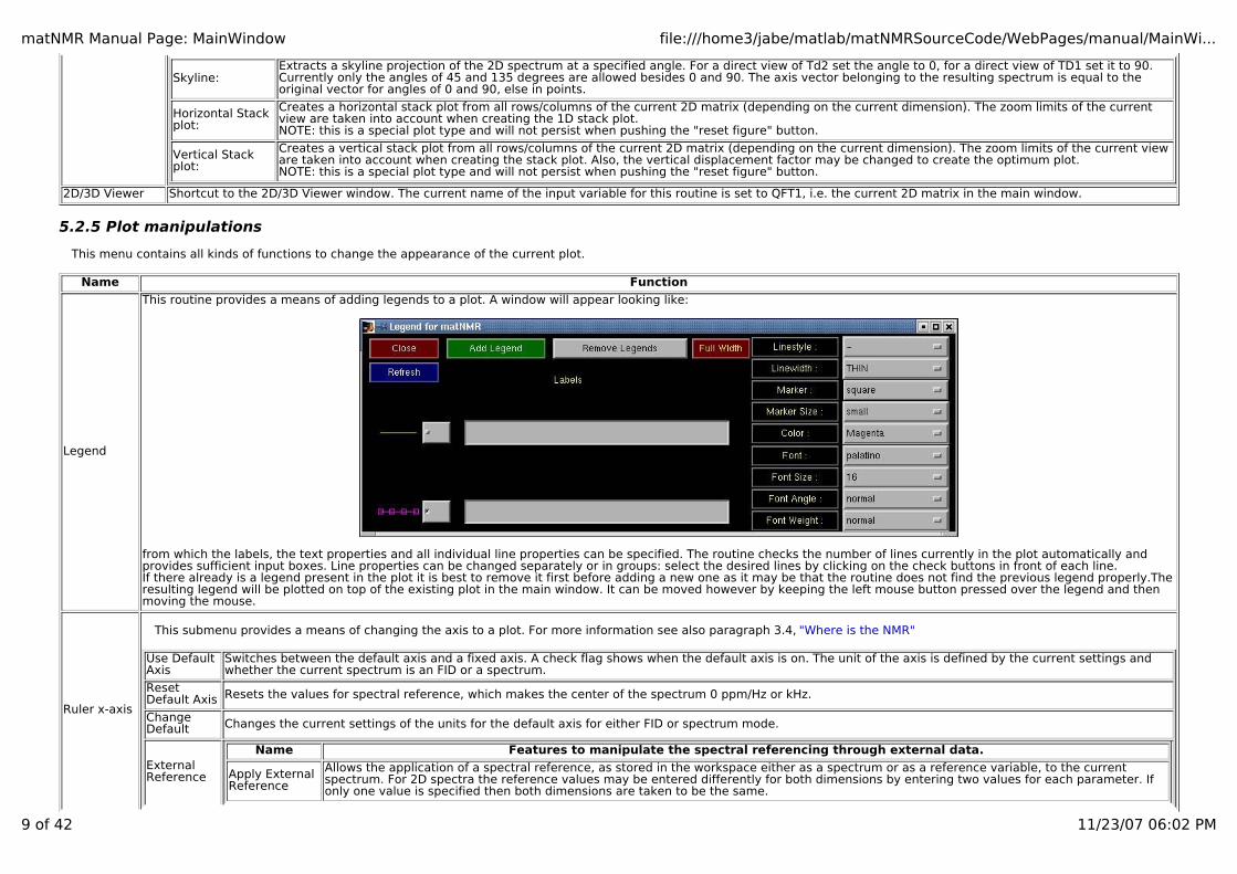
matNMR Manual Page: MainWindow file:///home3/jabe/matlab/matNMRSourceCode/WebPages/manual/MainWi...
9 of 42 11/23/07 06:02 PM
Skyline:Extracts a skyline projection of the 2D spectrum at a specified angle. For a direct view of Td2 set the angle to 0, for a direct view of TD1 set it to 90.Currently only the angles of 45 and 135 degrees are allowed besides 0 and 90. The axis vector belonging to the resulting spectrum is equal to theoriginal vector for angles of 0 and 90, else in points.
Horizontal Stack plot:
Creates a horizontal stack plot from all rows/columns of the current 2D matrix (depending on the current dimension). The zoom limits of the currentview are taken into account when creating the 1D stack plot. NOTE: this is a special plot type and will not persist when pushing the "reset figure" button.
Vertical Stack plot:
Creates a vertical stack plot from all rows/columns of the current 2D matrix (depending on the current dimension). The zoom limits of the current vieware taken into account when creating the stack plot. Also, the vertical displacement factor may be changed to create the optimum plot. NOTE: this is a special plot type and will not persist when pushing the "reset figure" button.
2D/3D Viewer Shortcut to the 2D/3D Viewer window. The current name of the input variable for this routine is set to QFT1, i.e. the current 2D matrix in the main window.
5.2.5 Plot manipulations
This menu contains all kinds of functions to change the appearance of the current plot.
Name Function
Legend
This routine provides a means of adding legends to a plot. A window will appear looking like:
from which the labels, the text properties and all individual line properties can be specified. The routine checks the number of lines currently in the plot automatically andprovides sufficient input boxes. Line properties can be changed separately or in groups: select the desired lines by clicking on the check buttons in front of each line.If there already is a legend present in the plot it is best to remove it first before adding a new one as it may be that the routine does not find the previous legend properly.Theresulting legend will be plotted on top of the existing plot in the main window. It can be moved however by keeping the left mouse button pressed over the legend and thenmoving the mouse.
Ruler x-axis
This submenu provides a means of changing the axis to a plot. For more information see also paragraph 3.4, "Where is the NMR"
Use Default Axis
Switches between the default axis and a fixed axis. A check flag shows when the default axis is on. The unit of the axis is defined by the current settings andwhether the current spectrum is an FID or a spectrum.
Reset Default Axis Resets the values for spectral reference, which makes the center of the spectrum 0 ppm/Hz or kHz.
Change Default Changes the current settings of the units for the default axis for either FID or spectrum mode.
External Reference
Name Features to manipulate the spectral referencing through external data.
Apply External Reference
Allows the application of a spectral reference, as stored in the workspace either as a spectrum or as a reference variable, to the currentspectrum. For 2D spectra the reference values may be entered differently for both dimensions by entering two values for each parameter. Ifonly one value is specified then both dimensions are taken to be the same.

matNMR Manual Page: MainWindow file:///home3/jabe/matlab/matNMRSourceCode/WebPages/manual/MainWi...
10 of 42 11/23/07 06:02 PM
Define External Reference
Allows manual definition of a spectral reference. For 2D spectra the reference values may be entered differently for both dimensions byentering two values for each parameter. If only one value is specified then both dimensions are taken to be the same.
Import External Reference
Allows importing of a spectral reference from an external dataset. This requires the default axis mode is on AND that all spectral parametersfor the current dataset have been set correctly. Especially the sign of gamma (magnetogyric ratio) is important as this will determine the signof a frequency axis. NOTE that both XWinNMR and Spinsight do not handle this correctly and that the sign may therefore be different.Currently this only works for the XWinNMR, VNMR and Spinsight formats but should be implemented for other formats as well at some point(kick me to speed up this process!)
Other
The rest of the menu allows direct access to axes in time, gradient, points or a user-defined vector, but also to the menu-based option "ruler X-axis". A windowwill appear looking like:
from which the type of axis vector (PPM, kHz, Hz, time, gradient, points, user-defined) can be chosen. The spectral width must be specified for PPM and Hz axesand for a PPM axis also the carrier frequency. For an axis in Hz also the sign of the gyromagnetic ratio of the nucleus that corresponds to the current spectrummust be specified. NOTE: Gradient axes are defined in T/m and NOT in G/cm. This means you may have to divide the gradient values from your software by 100to obtain the proper values!! Pressing the "Continue" button proceeds the routine and one is asked for a reference value. After that the reference peak can be specified by using thecrosshair mouse pounter and clicking on the desired reference peak (This may seem strange but is necessary because of a MATLAB bug. Specifying thereference peak before asking its value leads to a mess with the main and input window). If a name is given for the new axis vector then it will be saved in theworkspace after calculating it.
Title/axis labels
This routine provides a means of changing the title and axes labels of a plot. A window will appear looking like:
Pressing the "Apply" button will update all labels immediately. The "Refresh" is used for updating the text labels currently written in this window to the labels in the currentplot (useful when having this window opened continously). The "full width" button expands the window to the full width of the screen to give wider edit buttons. This is usefulfor long texts as they can become inaccessible because the scrolling doesn't work perfectly.
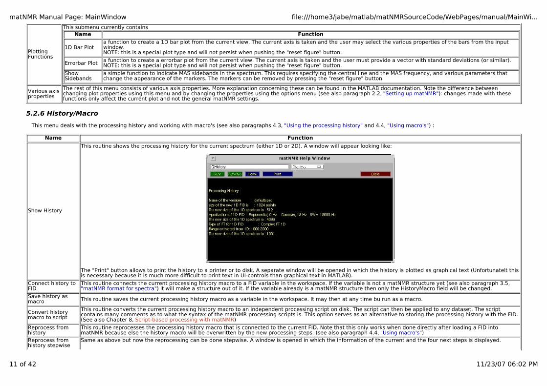
matNMR Manual Page: MainWindow file:///home3/jabe/matlab/matNMRSourceCode/WebPages/manual/MainWi...
11 of 42 11/23/07 06:02 PM
Plotting Functions
This submenu currently containsName Function
1D Bar Plota function to create a 1D bar plot from the current view. The current axis is taken and the user may select the various properties of the bars from the inputwindow. NOTE: this is a special plot type and will not persist when pushing the "reset figure" button.
Errorbar Plot a function to create a errorbar plot from the current view. The current axis is taken and the user must provide a vector with standard deviations (or similar). NOTE: this is a special plot type and will not persist when pushing the "reset figure" button.
Show Sidebands
a simple function to indicate MAS sidebands in the spectrum. This requires specifying the central line and the MAS frequency, and various parameters thatchange the appearance of the markers. The markers can be removed by pressing the "reset figure" button.
Various axis properties
The rest of this menu consists of various axis properties. More explanation concerning these can be found in the MATLAB documentation. Note the difference betweenchanging plot properties using this menu and by changing the properties using the options menu (see also paragraph 2.2, "Setting up matNMR"): changes made with thesefunctions only affect the current plot and not the general matNMR settings.
5.2.6 History/Macro
This menu deals with the processing history and working with macro's (see also paragraphs 4.3, "Using the processing history" and 4.4, "Using macro's") :
Name Function
Show History
This routine shows the processing history for the current spectrum (either 1D or 2D). A window will appear looking like:
The "Print" button allows to print the history to a printer or to disk. A separate window will be opened in which the history is plotted as graphical text (Unfortunatelt thisis necessary because it is much more difficult to print text in UI-controls than graphical text in MATLAB).
Connect history to FID
This routine connects the current processing history macro to a FID variable in the workspace. If the variable is not a matNMR structure yet (see also paragraph 3.5,"matNMR format for spectra") it will make a structure out of it. If the variable already is a matNMR structure then only the HistoryMacro field will be changed.
Save history as macro This routine saves the current processing history macro as a variable in the workspace. It may then at any time bu run as a macro.
Convert history macro to script
This routine converts the current processing history macro to an independent processing script on disk. The script can then be applied to any dataset. The scriptcontains many comments as to what the syntax of the matNMR processing scripts is. This option serves as an alternative to storing the processing history with the FID.(See also Chapter 8, Script-based processing with matNMR)
Reprocess from history
This routine reprocesses the processing history macro that is connected to the current FID. Note that this only works when done directly after loading a FID intomatNMR because else the history macro will be overwritten by the new processing steps. (see also paragraph 4.4, "Using macro's")
Reprocess from history stepwise
Same as above but now the reprocessing can be done stepwise. A window is opened in which the information of the current and the four next steps is displayed.
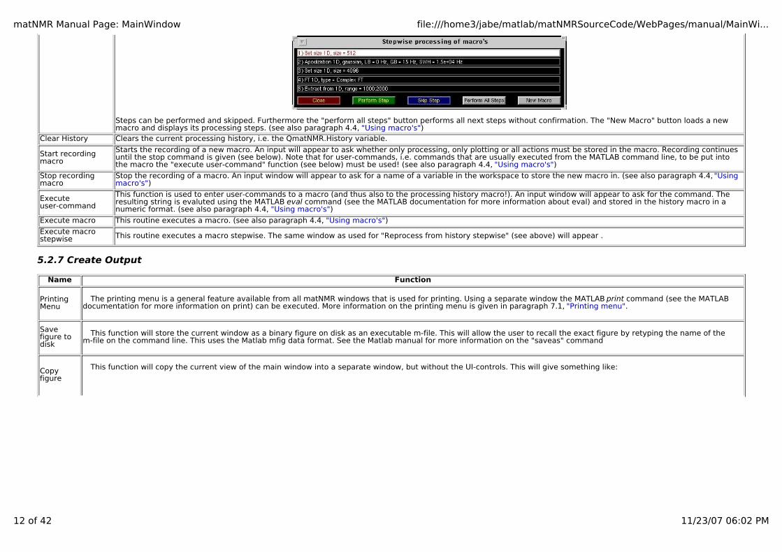
matNMR Manual Page: MainWindow file:///home3/jabe/matlab/matNMRSourceCode/WebPages/manual/MainWi...
12 of 42 11/23/07 06:02 PM
Steps can be performed and skipped. Furthermore the "perform all steps" button performs all next steps without confirmation. The "New Macro" button loads a newmacro and displays its processing steps. (see also paragraph 4.4, "Using macro's")
Clear History Clears the current processing history, i.e. the QmatNMR.History variable.
Start recording macro
Starts the recording of a new macro. An input will appear to ask whether only processing, only plotting or all actions must be stored in the macro. Recording continuesuntil the stop command is given (see below). Note that for user-commands, i.e. commands that are usually executed from the MATLAB command line, to be put intothe macro the "execute user-command" function (see below) must be used! (see also paragraph 4.4, "Using macro's")
Stop recording macro
Stop the recording of a macro. An input window will appear to ask for a name of a variable in the workspace to store the new macro in. (see also paragraph 4.4, "Using macro's")
Execute user-command
This function is used to enter user-commands to a macro (and thus also to the processing history macro!). An input window will appear to ask for the command. Theresulting string is evaluted using the MATLAB eval command (see the MATLAB documentation for more information about eval) and stored in the history macro in anumeric format. (see also paragraph 4.4, "Using macro's")
Execute macro This routine executes a macro. (see also paragraph 4.4, "Using macro's")
Execute macro stepwise This routine executes a macro stepwise. The same window as used for "Reprocess from history stepwise" (see above) will appear .
5.2.7 Create Output
Name Function
Printing Menu
The printing menu is a general feature available from all matNMR windows that is used for printing. Using a separate window the MATLAB print command (see the MATLAB documentation for more information on print) can be executed. More information on the printing menu is given in paragraph 7.1, "Printing menu".
Save figure to disk
This function will store the current window as a binary figure on disk as an executable m-file. This will allow the user to recall the exact figure by retyping the name of them-file on the command line. This uses the Matlab mfig data format. See the Matlab manual for more information on the "saveas" command
Copy figure
This function will copy the current view of the main window into a separate window, but without the UI-controls. This will give something like:
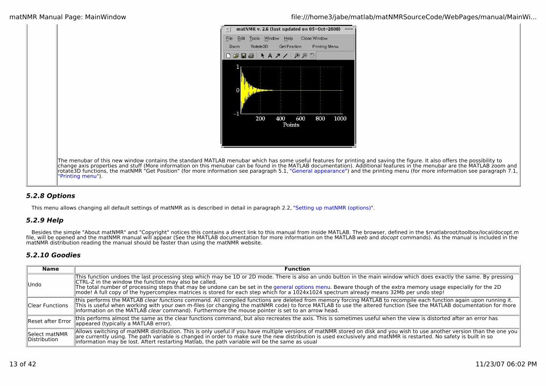
matNMR Manual Page: MainWindow file:///home3/jabe/matlab/matNMRSourceCode/WebPages/manual/MainWi...
13 of 42 11/23/07 06:02 PM
The menubar of this new window contains the standard MATLAB menubar which has some useful features for printing and saving the figure. It also offers the possibility tochange axis properties and stuff (More information on this menubar can be found in the MATLAB documentation). Additional features in the menubar are the MATLAB zoom androtate3D functions, the matNMR "Get Position" (for more information see paragraph 5.1, "General appearance") and the printing menu (for more information see paragraph 7.1,"Printing menu").
5.2.8 Options
This menu allows changing all default settings of matNMR as is described in detail in paragraph 2.2, "Setting up matNMR (options)".
5.2.9 Help
Besides the simple "About matNMR" and "Copyright" notices this contains a direct link to this manual from inside MATLAB. The browser, defined in the $matlabroot/toolbox/local/docopt.mfile, will be opened and the matNMR manual will appear (See the MATLAB documentation for more information on the MATLAB web and docopt commands). As the manual is included in the matNMR distribution reading the manual should be faster than using the matNMR website.
5.2.10 Goodies
Name Function
Undo
This function undoes the last processing step which may be 1D or 2D mode. There is also an undo button in the main window which does exactly the same. By pressingCTRL-Z in the window the function may also be called. The total number of processing steps that may be undone can be set in the general options menu. Beware though of the extra memory usage especially for the 2Dmode! A full copy of the hypercomplex matrices is stored for each step which for a 1024x1024 spectrum already means 32Mb per undo step!
Clear Functionsthis performs the MATLAB clear functions command. All compiled functions are deleted from memory forcing MATLAB to recompile each function again upon running it.This is useful when working with your own m-files (or changing the matNMR code) to force MATLAB to use the altered function (See the MATLAB documentation for moreinformation on the MATLAB clear command). Furthermore the mouse pointer is set to an arrow head.
Reset after Error this performs almost the same as the clear functions command, but also recreates the axis. This is sometimes useful when the view is distorted after an error hasappeared (typically a MATLAB error).
Select matNMR Distribution
Allows switching of matNMR distribution. This is only useful if you have multiple versions of matNMR stored on disk and you wish to use another version than the one youare currently using. The path variable is changed in order to make sure the new distribution is used exclusively and matNMR is restarted. No safety is built in soinformation may be lost. Aftert restarting Matlab, the path variable will be the same as usual

matNMR Manual Page: MainWindow file:///home3/jabe/matlab/matNMRSourceCode/WebPages/manual/MainWi...
14 of 42 11/23/07 06:02 PM
5.3 Fitting of CSA tensors from the MAS sideband manifold
5.3.1 General appearance
MatNMR offers a fitting routine for magic-angle spinning sideband intensities from the "1D Processing" entry in the menubar. The following figure window will appear:
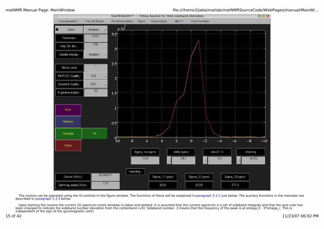
matNMR Manual Page: MainWindow file:///home3/jabe/matlab/matNMRSourceCode/WebPages/manual/MainWi...
15 of 42 11/23/07 06:02 PM
The routine can be operated using the UI-controls in the figure window. The functions of these will be explained in paragraph 5.3.2 just below. The auxilary functions in the menubar aredescribed in paragraph 5.3.3 below.
Upon starting the routine the current 1D spectrum (main window) is taken and plotted. It is assumed that the current spectrum is a set of sideband integrals and that the axis ruler hasbeen changed to indicate the sideband number deviation from the centerband (=0). Sideband number -3 means that the frequency of the peak is at omega_0 - 3*omega_r. This isindependent of the sign of the gyromagnetic ratio!

matNMR Manual Page: MainWindow file:///home3/jabe/matlab/matNMRSourceCode/WebPages/manual/MainWi...
16 of 42 11/23/07 06:02 PM
To best way to obtain the sideband amplitudes is to use the deconvolution routine, paragraph 5.6 to fit the lineshapes of the individual sidebands, and take the values for the integrals anduse them for the fit of the sideband amplitudes. This is more accurate than taking only the intensity of the line at a multiple of the spinning speed, since spinning speed instabilities willhardly affect the centerband but the increasingly affect the line for higher sideband numbers. The integral of the line should not be affected. After fitting the 1D spectrum, the results arestored in a structure and one of the fields is called "Integrals". These contain the values for the peaks. Add the correct axis for the sideband numbers, taking care that the sign of thegyromagnetic ratio is correct. Otherwise the sign of the anisotropy delta will invert.
To fit the sideband manifold, the Larmor frequency must be entered in MHz and the magic-angle spinning frequency in kHz. The isotropic shift in ppm may also be entered if tensor valuessigma_11, sigma_22 and sigma_33 are required. The routine itself only fits the anisotropy "delta" and the asymmetry "eta", and an intensity. The sideband manifold is calculated using agammaCOMPUTE-based algorithm which uses an analytical expression for the frequency of a crystallite. Through powder averaging the complete sideband manifold can be calculated.
As holds for all non-linear fits a good initial estimate of the parameters is required for an efficient fit convergence. To facilitate finding such an estimate the "Simulate" button may beused. After having defined the initial guesses the fit can be started with the "Fit" button. Should a parameter not be fitted but kept constant at its current value, then this can be done byselecting the check button (with the square block in it) belonging to the parameter.
Two algorithms may be used for fitting: SIMPLEX and a gradient algorithm. Typically the SIMPLEX algorithm is used for coarse optimization and is followed by a gradient minimization tofinish off the analysis. The quality of the simulation of the sideband manifold can be determined for both algorithms separately. The simulation uses a gammaCOMPUTE-based calculationwith a two-angle ZCW scheme for angles alpha and beta, and a separate number of angles gamma, which can be selected in the appropriate UIcontrol. By choosing a higher number ofpowder-averaging angles the quality of the simulation will improve. By default 610 powder-averaging angles are selected for SIMPLEX and none for the gradient algorithm. The value of 610angles, combined with 50 values for angle gamma seems to provide a stable and fast result for a wide number of conditions (say up to 10 sidebands at least). When more sidebands arerequired it is important to test the stability of the fit by increasing the number of averaging points.
When the fit has finished by default the results are written into the variable QSSAFitResults which can be read out by hand by the user (Note that this variable will be deleted whenmatNMR is stopped! This means it must be renamed, if it has to be kept in the workspace for later use, before stopping matNMR). Alternatively, from the "View Fit Results" entry in themenubar a new name for putting the results in can be defined. To be able to access this variable the user must make the variable global by typing "global VariableName" at the MATLABprompt. A message is written to make sure the user doesn't forget this.The format of the parameters is as follows:
- delta- eta- intensity- Error- Carrier- Spinning Speed- isotropic shiftAll these numbers are put in a single row. This variable is combined with the original data, the axis to the data, the fitted spectrum and the error value into a structure variable. The fields inthis variable are "Parameters", "Fit", "Data", "Axis" and "Error".
5.3.2 Buttons
Name Function
Zoom Switches the zoom function on or off.
Verbose Determines the level of output generated by the fitting algorithms. This can either be never, after every iteration or only after finishing the fit.
Tolerance Termination tolerance for the fit.
Max. Nr. Iter. Maximum number of iterations for each fit.
Update display Defines whether the plot should be updated after each iteration or only after the fit has finished.
Noise level In order for the calculated error to be a chi^2 the standard deviation of the noise must be entered here. This can be taken from the 1D spectrum. A proper value for thenoise level should ideally result in an error of 1 for a perfect fit, i.e. the residual is nothing more than the standard deviation of the noise then.
SIMPLEX quality
Number of powder-averaging points for the SIMPLEX algorithm. A two-angle ZCW grid is used during the simulation. Selecting "OFF" will result in the algorithm not beingused. Increase this value for a more accurate result.
Gradient quality
Number of powder-averaging points for the gradient algorithm. A two-angle ZCW grid is used during the simulation. Selecting "OFF" will result in the algorithm not beingused. Increase this value for a more accurate result.
# gamma angles
Defines the number of angles gamma for the powder averaging. This should be larger than the maximum sideband number that needs to be extracted. 50 seems to be agood value for most practical cases (up to +- 10 sidebands) as it results in a stable simulation. Increase this value for a more accurate result.
Print Prints the current figure window to the the default printer as defined in the $matlabroot/toolbox/local/printopt.m file. No UI-controls are printed as the parameter values areput into the plot as white text. The resulting plot can be rather ugly as sometimes the text is right on top of the fitted spectrum.
Refresh Uploads the current 1D spectrum from the main window into the fitting routine.
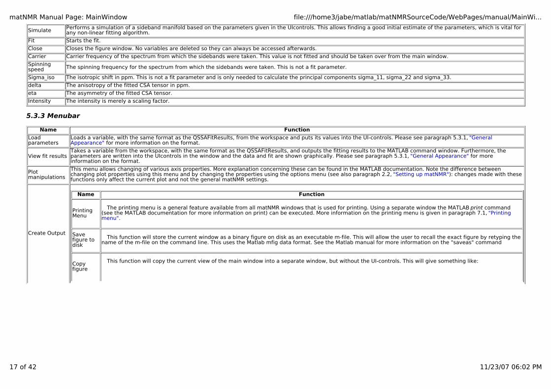
matNMR Manual Page: MainWindow file:///home3/jabe/matlab/matNMRSourceCode/WebPages/manual/MainWi...
17 of 42 11/23/07 06:02 PM
Simulate Performs a simulation of a sideband manifold based on the parameters given in the UIcontrols. This allows finding a good initial estimate of the parameters, which is vital forany non-linear fitting algorithm.
Fit Starts the fit.
Close Closes the figure window. No variables are deleted so they can always be accessed afterwards.
Carrier Carrier frequency of the spectrum from which the sidebands were taken. This value is not fitted and should be taken over from the main window.
Spinning speed The spinning frequency for the spectrum from which the sidebands were taken. This is not a fit parameter.
Sigma_iso The isotropic shift in ppm. This is not a fit parameter and is only needed to calculate the principal components sigma_11, sigma_22 and sigma_33.
delta The anisotropy of the fitted CSA tensor in ppm.
eta The asymmetry of the fitted CSA tensor.
Intensity The intensity is merely a scaling factor.
5.3.3 Menubar
Name Function
Load parameters
Loads a variable, with the same format as the QSSAFitResults, from the workspace and puts its values into the UI-controls. Please see paragraph 5.3.1, "General Appearance" for more information on the format.
View fit resultsTakes a variable from the workspace, with the same format as the QSSAFitResults, and outputs the fitting results to the MATLAB command window. Furthermore, theparameters are written into the UIcontrols in the window and the data and fit are shown graphically. Please see paragraph 5.3.1, "General Appearance" for more information on the format.
Plot manipulations
This menu allows changing of various axis properties. More explanation concerning these can be found in the MATLAB documentation. Note the difference betweenchanging plot properties using this menu and by changing the properties using the options menu (see also paragraph 2.2, "Setting up matNMR"): changes made with thesefunctions only affect the current plot and not the general matNMR settings.
Create Output
Name Function
Printing Menu
The printing menu is a general feature available from all matNMR windows that is used for printing. Using a separate window the MATLAB print command (see the MATLAB documentation for more information on print) can be executed. More information on the printing menu is given in paragraph 7.1, "Printing menu".
Save figure to disk
This function will store the current window as a binary figure on disk as an executable m-file. This will allow the user to recall the exact figure by retyping thename of the m-file on the command line. This uses the Matlab mfig data format. See the Matlab manual for more information on the "saveas" command
Copy figure
This function will copy the current view of the main window into a separate window, but without the UI-controls. This will give something like:

matNMR Manual Page: MainWindow file:///home3/jabe/matlab/matNMRSourceCode/WebPages/manual/MainWi...
18 of 42 11/23/07 06:02 PM
The menubar of this new window contains the standard MATLAB menubar which has some useful features for printing and saving the figure. It also offers thepossibility to change axis properties and stuff (More information on this menubar can be found in the MATLAB documentation). Additional features in themenubar are the MATLAB zoom and rotate3D functions, the matNMR "Get Position" (for more information see paragraph 5.1, "General appearance") and theprinting menu (for more information see paragraph 7.1, "Printing menu").
Macro
Name Function
Start recording macro
Starts the recording of a new macro. An input will appear to ask whether only processing, only plotting or all actions must be stored in the macro.Recording continues until the stop command is given (see below). Note that for user-commands, i.e. commands that are usually executed from theMATLAB command line, to be put into the macro the "execute user-command" function (see below) must be used! (see also paragraph 4.4, "Using macro's")
Stop recording macro
Stop the recording of a macro. An input window will appear to ask for a name of a variable in the workspace to store the new macro in. (see also paragraph4.4, "Using macro's")
Execute macro This routine executes a macro. (see also paragraph 4.4, "Using macro's")
Execute macro stepwise
This routine executes a macro stepwise. The same window as used for "Reprocess from history stepwise" (see above) will appear .
Help?Besides the simple "About matNMR" and "Copyright" notices this contains a direct link to this manual from inside MATLAB. The browser, defined in the$matlabroot/toolbox/local/docopt.m file, will be opened and the matNMR manual will appear (See the MATLAB documentation for more information on the MATLAB web anddocopt commands). As the manual is included in the matNMR distribution reading the manual should be faster than using the matNMR website.
Clear functionsThis performs the MATLAB "clear functions" command. All compiled functions are deleted from memory forcing MATLAB to recompile each function again upon running it.This is useful when working with your own m-files (or changing the matNMR code) to force MATLAB to use the altered function (See the MATLAB documentation for moreinformation on the MATLAB clear command). Furthermore the mouse pointer is set to an arrow head.
matNMR Manual Page: MainWindow file:///home3/jabe/matlab/matNMRSourceCode/WebPages/manual/MainWi...
19 of 42 11/23/07 06:02 PM
5.4 Fitting of CSA tensors from static powder patterns
5.4.1 General appearance
MatNMR offers a fitting routine for CSA tensors from static powder spectra which can be accessed from the "1D Processing" entry in the menubar. The following figure window will appear:
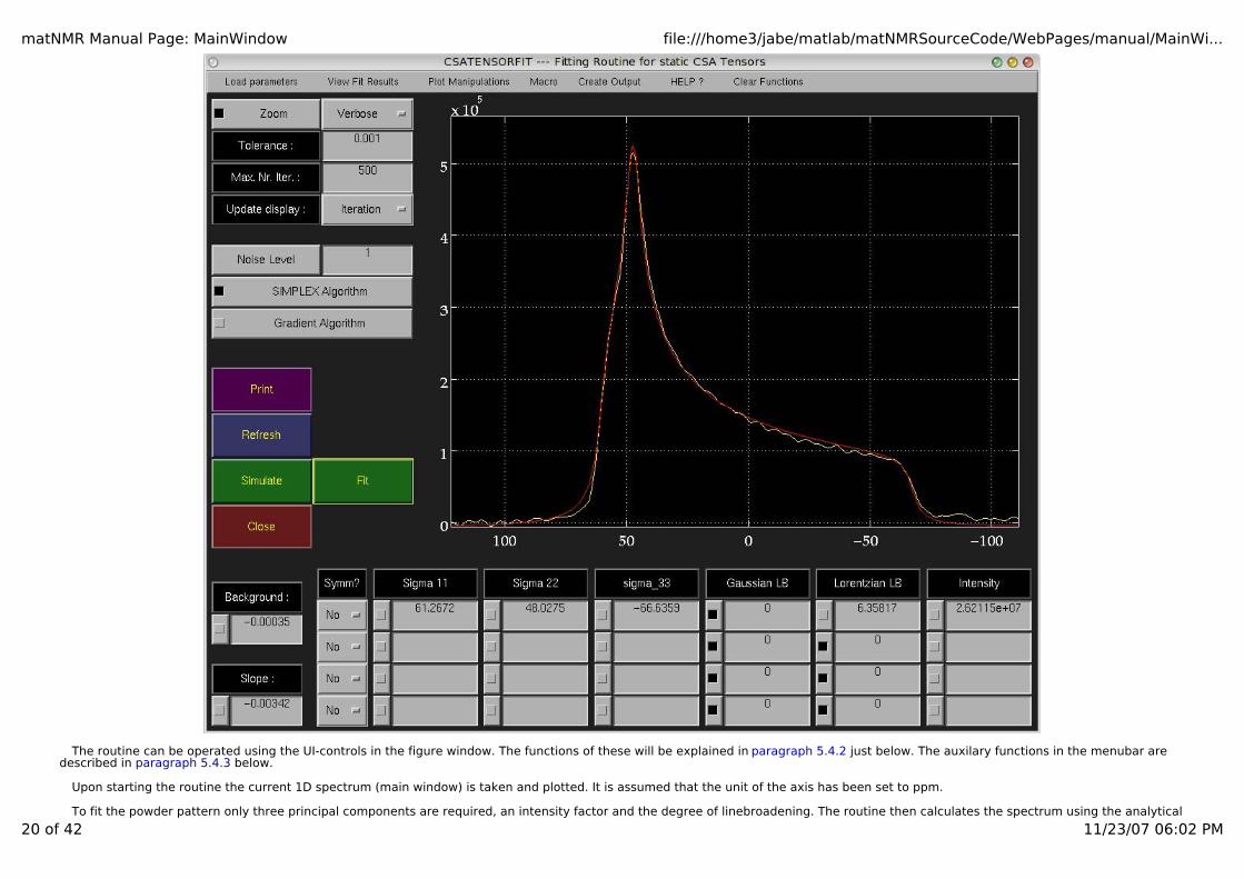
matNMR Manual Page: MainWindow file:///home3/jabe/matlab/matNMRSourceCode/WebPages/manual/MainWi...
20 of 42 11/23/07 06:02 PM
The routine can be operated using the UI-controls in the figure window. The functions of these will be explained in paragraph 5.4.2 just below. The auxilary functions in the menubar aredescribed in paragraph 5.4.3 below.
Upon starting the routine the current 1D spectrum (main window) is taken and plotted. It is assumed that the unit of the axis has been set to ppm.
To fit the powder pattern only three principal components are required, an intensity factor and the degree of linebroadening. The routine then calculates the spectrum using the analytical
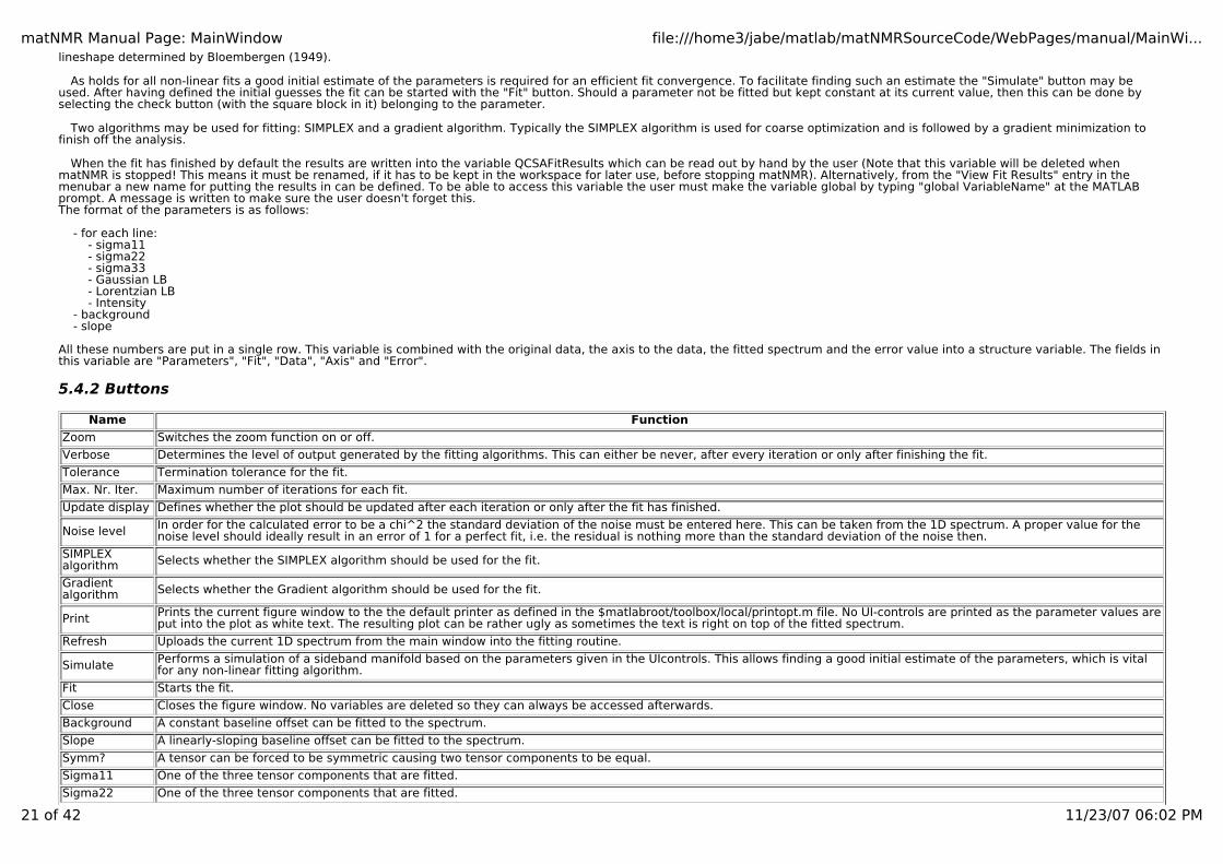
matNMR Manual Page: MainWindow file:///home3/jabe/matlab/matNMRSourceCode/WebPages/manual/MainWi...
21 of 42 11/23/07 06:02 PM
lineshape determined by Bloembergen (1949).
As holds for all non-linear fits a good initial estimate of the parameters is required for an efficient fit convergence. To facilitate finding such an estimate the "Simulate" button may beused. After having defined the initial guesses the fit can be started with the "Fit" button. Should a parameter not be fitted but kept constant at its current value, then this can be done byselecting the check button (with the square block in it) belonging to the parameter.
Two algorithms may be used for fitting: SIMPLEX and a gradient algorithm. Typically the SIMPLEX algorithm is used for coarse optimization and is followed by a gradient minimization tofinish off the analysis.
When the fit has finished by default the results are written into the variable QCSAFitResults which can be read out by hand by the user (Note that this variable will be deleted whenmatNMR is stopped! This means it must be renamed, if it has to be kept in the workspace for later use, before stopping matNMR). Alternatively, from the "View Fit Results" entry in themenubar a new name for putting the results in can be defined. To be able to access this variable the user must make the variable global by typing "global VariableName" at the MATLABprompt. A message is written to make sure the user doesn't forget this.The format of the parameters is as follows:
- for each line: - sigma11 - sigma22 - sigma33 - Gaussian LB - Lorentzian LB - Intensity - background - slope
All these numbers are put in a single row. This variable is combined with the original data, the axis to the data, the fitted spectrum and the error value into a structure variable. The fields inthis variable are "Parameters", "Fit", "Data", "Axis" and "Error".
5.4.2 Buttons
Name Function
Zoom Switches the zoom function on or off.
Verbose Determines the level of output generated by the fitting algorithms. This can either be never, after every iteration or only after finishing the fit.
Tolerance Termination tolerance for the fit.
Max. Nr. Iter. Maximum number of iterations for each fit.
Update display Defines whether the plot should be updated after each iteration or only after the fit has finished.
Noise level In order for the calculated error to be a chi^2 the standard deviation of the noise must be entered here. This can be taken from the 1D spectrum. A proper value for thenoise level should ideally result in an error of 1 for a perfect fit, i.e. the residual is nothing more than the standard deviation of the noise then.
SIMPLEX algorithm Selects whether the SIMPLEX algorithm should be used for the fit.
Gradient algorithm Selects whether the Gradient algorithm should be used for the fit.
Print Prints the current figure window to the the default printer as defined in the $matlabroot/toolbox/local/printopt.m file. No UI-controls are printed as the parameter values areput into the plot as white text. The resulting plot can be rather ugly as sometimes the text is right on top of the fitted spectrum.
Refresh Uploads the current 1D spectrum from the main window into the fitting routine.
Simulate Performs a simulation of a sideband manifold based on the parameters given in the UIcontrols. This allows finding a good initial estimate of the parameters, which is vitalfor any non-linear fitting algorithm.
Fit Starts the fit.
Close Closes the figure window. No variables are deleted so they can always be accessed afterwards.
Background A constant baseline offset can be fitted to the spectrum.
Slope A linearly-sloping baseline offset can be fitted to the spectrum.
Symm? A tensor can be forced to be symmetric causing two tensor components to be equal.
Sigma11 One of the three tensor components that are fitted.
Sigma22 One of the three tensor components that are fitted.
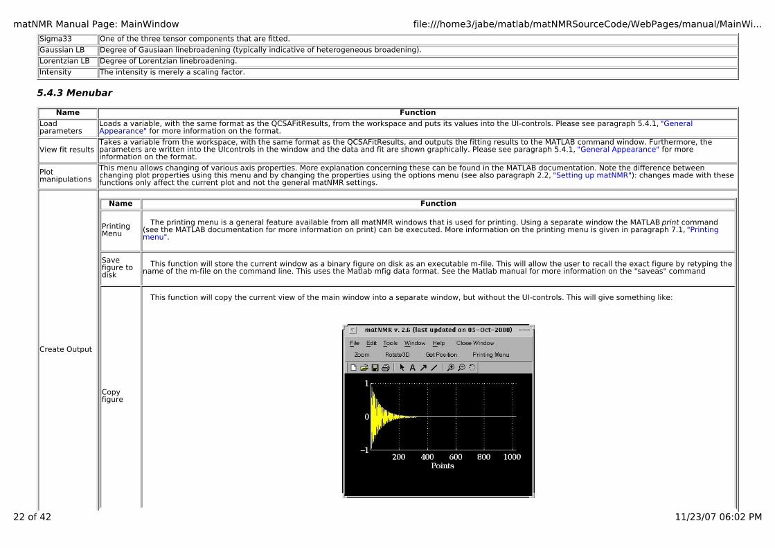
matNMR Manual Page: MainWindow file:///home3/jabe/matlab/matNMRSourceCode/WebPages/manual/MainWi...
22 of 42 11/23/07 06:02 PM
Sigma33 One of the three tensor components that are fitted.
Gaussian LB Degree of Gausiaan linebroadening (typically indicative of heterogeneous broadening).
Lorentzian LB Degree of Lorentzian linebroadening.
Intensity The intensity is merely a scaling factor.
5.4.3 Menubar
Name Function
Load parameters
Loads a variable, with the same format as the QCSAFitResults, from the workspace and puts its values into the UI-controls. Please see paragraph 5.4.1, "General Appearance" for more information on the format.
View fit resultsTakes a variable from the workspace, with the same format as the QCSAFitResults, and outputs the fitting results to the MATLAB command window. Furthermore, theparameters are written into the UIcontrols in the window and the data and fit are shown graphically. Please see paragraph 5.4.1, "General Appearance" for more information on the format.
Plot manipulations
This menu allows changing of various axis properties. More explanation concerning these can be found in the MATLAB documentation. Note the difference betweenchanging plot properties using this menu and by changing the properties using the options menu (see also paragraph 2.2, "Setting up matNMR"): changes made with thesefunctions only affect the current plot and not the general matNMR settings.
Create Output
Name Function
Printing Menu
The printing menu is a general feature available from all matNMR windows that is used for printing. Using a separate window the MATLAB print command (see the MATLAB documentation for more information on print) can be executed. More information on the printing menu is given in paragraph 7.1, "Printing menu".
Save figure to disk
This function will store the current window as a binary figure on disk as an executable m-file. This will allow the user to recall the exact figure by retyping thename of the m-file on the command line. This uses the Matlab mfig data format. See the Matlab manual for more information on the "saveas" command
Copy figure
This function will copy the current view of the main window into a separate window, but without the UI-controls. This will give something like:
matNMR Manual Page: MainWindow file:///home3/jabe/matlab/matNMRSourceCode/WebPages/manual/MainWi...
23 of 42 11/23/07 06:02 PM
The menubar of this new window contains the standard MATLAB menubar which has some useful features for printing and saving the figure. It also offers thepossibility to change axis properties and stuff (More information on this menubar can be found in the MATLAB documentation). Additional features in themenubar are the MATLAB zoom and rotate3D functions, the matNMR "Get Position" (for more information see paragraph 5.1, "General appearance") and theprinting menu (for more information see paragraph 7.1, "Printing menu").
Macro
Name Function
Start recording macro
Starts the recording of a new macro. An input will appear to ask whether only processing, only plotting or all actions must be stored in the macro.Recording continues until the stop command is given (see below). Note that for user-commands, i.e. commands that are usually executed from theMATLAB command line, to be put into the macro the "execute user-command" function (see below) must be used! (see also paragraph 4.4, "Using macro's")
Stop recording macro
Stop the recording of a macro. An input window will appear to ask for a name of a variable in the workspace to store the new macro in. (see also paragraph4.4, "Using macro's")
Execute macro This routine executes a macro. (see also paragraph 4.4, "Using macro's")
Execute macro stepwise
This routine executes a macro stepwise. The same window as used for "Reprocess from history stepwise" (see above) will appear .
Help?Besides the simple "About matNMR" and "Copyright" notices this contains a direct link to this manual from inside MATLAB. The browser, defined in the$matlabroot/toolbox/local/docopt.m file, will be opened and the matNMR manual will appear (See the MATLAB documentation for more information on the MATLAB web anddocopt commands). As the manual is included in the matNMR distribution reading the manual should be faster than using the matNMR website.
Clear functionsThis performs the MATLAB "clear functions" command. All compiled functions are deleted from memory forcing MATLAB to recompile each function again upon running it.This is useful when working with your own m-files (or changing the matNMR code) to force MATLAB to use the altered function (See the MATLAB documentation for moreinformation on the MATLAB clear command). Furthermore the mouse pointer is set to an arrow head.
5.5 Diffusion curve fitting
5.5.1 General appearance
MatNMR offers a basic isotropic pulsed-field gradient (PFG) curve fitting routine from the "1D Processing" entry in the menubar. The following figure window will appear:

matNMR Manual Page: MainWindow file:///home3/jabe/matlab/matNMRSourceCode/WebPages/manual/MainWi...
24 of 42 11/23/07 06:02 PM
The routine can be operated using the UI-controls in the figure window. The functions of these will be explained in paragraph 5.5.2 just below. The auxilary functions in the menubar aredescribed in paragraph 5.5.3 below.
Upon starting the routine the current 1D spectrum (main window) is taken and plotted. It is assumed that the axis ruler has been changed to a gradient axis, see paragraph 5.2.5. NOTE: Gradient axes are defined in T/m and NOT in G/cm. This means you may have to divide the gradient values from your software by 100 to obtain the propervalues!!

matNMR Manual Page: MainWindow file:///home3/jabe/matlab/matNMRSourceCode/WebPages/manual/MainWi...
25 of 42 11/23/07 06:02 PM
For a more convenient view on exponentials the vertical axis is plotted on a logarithmic scale. This can easily be changed using the "scaling types" item in the "plot manipulations" menu onthe menubar.
To fit a (multi-)exponential diffusion curve one first has to provide proper values for the three constants: the gyromagnetic ratio, the gradient spacing and the gradient duration. Bypushing the "Def. Pars." button an input window will be shown where the values can be given.
The next step is to make an initial guess for all exponential functions that need to be fitted to it. This can be done by typing the coefficient and the diffusion constant (D) for each fractionby hand into the corresponding UI-controls in the window. Also the overall amplitude and a constant may be defined. The routine will include a fraction into the fit if a coefficient value isspecified. Note that all parameters are given in the unit of the axis vector belonging to the current 1D spectrum. This means that the axis vector has to be defined before starting thepeak-fitting routine! A total of 4 exponentials can be fitted simultaneously.
After having defined the initial guesses the fit can be started with the "Fit" button. Should a parameter not be fitted but kept constant at its current value, then this can be done byselecting the check button (with the square block in it) belonging to the parameter.
When the fit has finished by default the results are written into the variable QDiffFitResults which can be read out by hand by the user (Note that this variable will be deleted whenmatNMR is stopped! This means it must be renamed, if it has to be kept in the workspace for later use, before stopping matNMR). Alternatively, from the "View Fit Results" entry in themenubar a new name for putting the results in can be defined. To be able to access this variable the user must make the variable global by typing "global VariableName" at the MATLABprompt. A message is written to make sure the user doesn't forget this.The format of the parameters is as follows:
- nr of iterations- chi2 for this column- fit parameters : - for each exponential: - Coefficient - Diffusion constant (D) - constant - amplitude
All these numbers are put in a single row. This variable is combined with the original data, the axis to the data, the fitted spectrum and the error value into a structure variable. The fields inthis variable are "Parameters", "Fit", "Data", "Axis" and "Error".
Last, in case the initial parameters are very far off the "Simplex prefit" check button may be activated. This makes matNMR use a SIMPLEX algorithm first before the gradient algorithm. Bydefault this option is active.
5.5.2 Buttons
Name Function
log plot Switches between a linear and a logarithmic y-axis.
Def. Pars.
Allows entering the gyromagnetic ratio, the gradient spacing and the gradient duration and optionally the length of the delay used in a bipolar gradient experiment to allowfor the switching of the gradients, all of which are needed for the fit. An input window will appear in which these parameters can be entered.Alternatively, if the data have been recorded on a Bruker spectrometer using the diff script provided for setting up diffusion experiments, instead of typing the values for thegradient spacing and the gradient duration one may select "READ Bruker" in the input window. Gamma still needs to be entered by hand though! NOTE that this only works from XWinNMR 3.0 since before 3.0 the diff script was different. Also, it may mean that this will change at some point.MatNMR will then ask for the corresponding "acqus" file for the data, from which the parameters d20, p17 and p18 are read. d20 corresponds to big DELTA. p17 is thegradient rise time and p18 the length of time at which the gradient is constant.
Fit Starts the fit.
Refresh Uploads the current 1D spectrum from the main window into the fitting routine.
Close Closes the figure window. No variables are deleted so they can always be accessed afterwards.
Print Prints the current figure window to the the default printer as defined in the $matlabroot/toolbox/local/printopt.m file. No UI-controls are printed as the parameter values areput into the plot as white text. The resulting plot can be rather ugly as sometimes the text is right on top of the fitted spectrum.
Redisplay no. Defines after how many iterations the plot must be redrawn. Set this to a high value to save time.
Max. Nr. Iter. Maximum number of iterations for each fit.
Tolerance Termination tolerance for the fit.
Sigma Measure for the noise in the data. When properly defined the error should become a true chi^2.
matNMR Manual Page: MainWindow file:///home3/jabe/matlab/matNMRSourceCode/WebPages/manual/MainWi...
26 of 42 11/23/07 06:02 PM
Ext. Output Flag for whether an extended output should be given. A detailed error analysis is presented. NOTE: the basic fitting routine has not been programmed by me and Ihave never checked the accuracy of the error analysis!
SIMPLEX prefit
Flag for whether the fit should use a SIMPLEX algorithm before the gradient algorithm. This reduces the common problem that the gradient algorithm doesn't find a properminimum when the parameters are too far off.
Amplitude Overall amplitude that scales the fit.
Constant A constant.
Coefficient Amplitude factor for the exponential fraction.
D Diffusion constant for the exponential fraction.
5.5.3 Menubar
Name Function
Load parameters
Loads a variable, with the same format as the QDiffFitResults, from the workspace and puts its values into the UI-controls. Please see paragraph 5.5.1, "General Appearance" for more information on the format.
View fit resultsTakes a variable from the workspace, with the same format as the QDiffFitResults, and outputs the fitting results to the MATLAB command window. Furthermore, theparameters are written into the UIcontrols in the window and the data and fit are shown graphically. Please see paragraph 5.5.1, "General Appearance" for more information on the format.
Plot manipulations
This menu allows changing of various axis properties. More explanation concerning these can be found in the MATLAB documentation. Note the difference betweenchanging plot properties using this menu and by changing the properties using the options menu (see also paragraph 2.2, "Setting up matNMR"): changes made with thesefunctions only affect the current plot and not the general matNMR settings.
Create Output
Name Function
Printing Menu
The printing menu is a general feature available from all matNMR windows that is used for printing. Using a separate window the MATLAB print command (see the MATLAB documentation for more information on print) can be executed. More information on the printing menu is given in paragraph 7.1, "Printing menu".
Save figure to disk
This function will store the current window as a binary figure on disk as an executable m-file. This will allow the user to recall the exact figure by retyping thename of the m-file on the command line. This uses the Matlab mfig data format. See the Matlab manual for more information on the "saveas" command
Copy figure
This function will copy the current view of the main window into a separate window, but without the UI-controls. This will give something like:

matNMR Manual Page: MainWindow file:///home3/jabe/matlab/matNMRSourceCode/WebPages/manual/MainWi...
27 of 42 11/23/07 06:02 PM
The menubar of this new window contains the standard MATLAB menubar which has some useful features for printing and saving the figure. It also offers thepossibility to change axis properties and stuff (More information on this menubar can be found in the MATLAB documentation). Additional features in themenubar are the MATLAB zoom and rotate3D functions, the matNMR "Get Position" (for more information see paragraph 5.1, "General appearance") and theprinting menu (for more information see paragraph 7.1, "Printing menu").
Macro
Name Function
Start recording macro
Starts the recording of a new macro. An input will appear to ask whether only processing, only plotting or all actions must be stored in the macro.Recording continues until the stop command is given (see below). Note that for user-commands, i.e. commands that are usually executed from theMATLAB command line, to be put into the macro the "execute user-command" function (see below) must be used! (see also paragraph 4.4, "Using macro's")
Stop recording macro
Stop the recording of a macro. An input window will appear to ask for a name of a variable in the workspace to store the new macro in. (see also paragraph4.4, "Using macro's")
Execute macro This routine executes a macro. (see also paragraph 4.4, "Using macro's")
Execute macro stepwise
This routine executes a macro stepwise. The same window as used for "Reprocess from history stepwise" (see above) will appear .
Help?Besides the simple "About matNMR" and "Copyright" notices this contains a direct link to this manual from inside MATLAB. The browser, defined in the$matlabroot/toolbox/local/docopt.m file, will be opened and the matNMR manual will appear (See the MATLAB documentation for more information on the MATLAB web anddocopt commands). As the manual is included in the matNMR distribution reading the manual should be faster than using the matNMR website.
Clear functionsThis performs the MATLAB "clear functions" command. All compiled functions are deleted from memory forcing MATLAB to recompile each function again upon running it.This is useful when working with your own m-files (or changing the matNMR code) to force MATLAB to use the altered function (See the MATLAB documentation for moreinformation on the MATLAB clear command). Furthermore the mouse pointer is set to an arrow head.

matNMR Manual Page: MainWindow file:///home3/jabe/matlab/matNMRSourceCode/WebPages/manual/MainWi...
28 of 42 11/23/07 06:02 PM
5.6 Peak Deconvolution (mixed Gaussian/Lorentzian lineshapes)
5.6.1 General appearance
MatNMR offers a basic peak-fitting routine from both "1D Processing" and "2D Processing" entries in the menubar. The following figure window will appear:
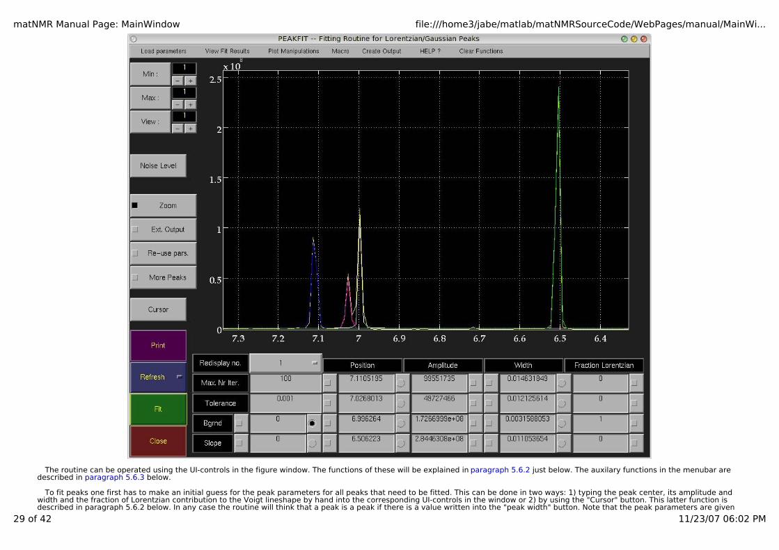
matNMR Manual Page: MainWindow file:///home3/jabe/matlab/matNMRSourceCode/WebPages/manual/MainWi...
29 of 42 11/23/07 06:02 PM
The routine can be operated using the UI-controls in the figure window. The functions of these will be explained in paragraph 5.6.2 just below. The auxilary functions in the menubar aredescribed in paragraph 5.6.3 below.
To fit peaks one first has to make an initial guess for the peak parameters for all peaks that need to be fitted. This can be done in two ways: 1) typing the peak center, its amplitude andwidth and the fraction of Lorentzian contribution to the Voigt lineshape by hand into the corresponding UI-controls in the window or 2) by using the "Cursor" button. This latter function isdescribed in paragraph 5.6.2 below. In any case the routine will think that a peak is a peak if there is a value written into the "peak width" button. Note that the peak parameters are given
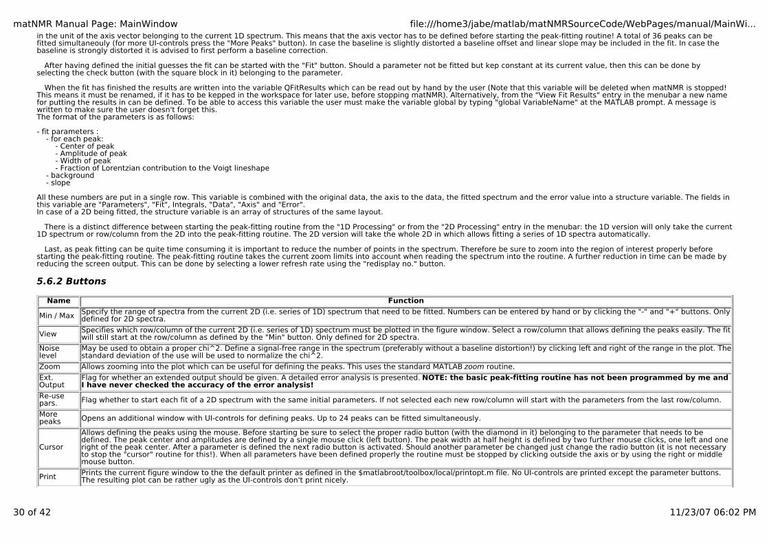
matNMR Manual Page: MainWindow file:///home3/jabe/matlab/matNMRSourceCode/WebPages/manual/MainWi...
30 of 42 11/23/07 06:02 PM
in the unit of the axis vector belonging to the current 1D spectrum. This means that the axis vector has to be defined before starting the peak-fitting routine! A total of 36 peaks can befitted simultaneouly (for more UI-controls press the "More Peaks" button). In case the baseline is slightly distorted a baseline offset and linear slope may be included in the fit. In case thebaseline is strongly distorted it is advised to first perform a baseline correction.
After having defined the initial guesses the fit can be started with the "Fit" button. Should a parameter not be fitted but kep constant at its current value, then this can be done byselecting the check button (with the square block in it) belonging to the parameter.
When the fit has finished the results are written into the variable QFitResults which can be read out by hand by the user (Note that this variable will be deleted when matNMR is stopped!This means it must be renamed, if it has to be kepped in the workspace for later use, before stopping matNMR). Alternatively, from the "View Fit Results" entry in the menubar a new namefor putting the results in can be defined. To be able to access this variable the user must make the variable global by typing "global VariableName" at the MATLAB prompt. A message iswritten to make sure the user doesn't forget this.The format of the parameters is as follows:
- fit parameters : - for each peak: - Center of peak - Amplitude of peak - Width of peak - Fraction of Lorentzian contribution to the Voigt lineshape - background - slope
All these numbers are put in a single row. This variable is combined with the original data, the axis to the data, the fitted spectrum and the error value into a structure variable. The fields inthis variable are "Parameters", "Fit", Integrals, "Data", "Axis" and "Error".In case of a 2D being fitted, the structure variable is an array of structures of the same layout.
There is a distinct difference between starting the peak-fitting routine from the "1D Processing" or from the "2D Processing" entry in the menubar: the 1D version will only take the current1D spectrum or row/column from the 2D into the peak-fitting routine. The 2D version will take the whole 2D in which allows fitting a series of 1D spectra automatically.
Last, as peak fitting can be quite time consuming it is important to reduce the number of points in the spectrum. Therefore be sure to zoom into the region of interest properly beforestarting the peak-fitting routine. The peak-fitting routine takes the current zoom limits into account when reading the spectrum into the routine. A further reduction in time can be made byreducing the screen output. This can be done by selecting a lower refresh rate using the "redisplay no." button.
5.6.2 Buttons
Name Function
Min / Max Specify the range of spectra from the current 2D (i.e. series of 1D) spectrum that need to be fitted. Numbers can be entered by hand or by clicking the "-" and "+" buttons. Onlydefined for 2D spectra.
View Specifies which row/column of the current 2D (i.e. series of 1D) spectrum must be plotted in the figure window. Select a row/column that allows defining the peaks easily. The fitwill still start at the row/column as defined by the "Min" button. Only defined for 2D spectra.
Noise level
May be used to obtain a proper chi^2. Define a signal-free range in the spectrum (preferably without a baseline distortion!) by clicking left and right of the range in the plot. Thestandard deviation of the use will be used to normalize the chi^2.
Zoom Allows zooming into the plot which can be useful for defining the peaks. This uses the standard MATLAB zoom routine.
Ext. Output
Flag for whether an extended output should be given. A detailed error analysis is presented. NOTE: the basic peak-fitting routine has not been programmed by me andI have never checked the accuracy of the error analysis!
Re-use pars. Flag whether to start each fit of a 2D spectrum with the same initial parameters. If not selected each new row/column will start with the parameters from the last row/column.
More peaks Opens an additional window with UI-controls for defining peaks. Up to 24 peaks can be fitted simultaneously.
Cursor
Allows defining the peaks using the mouse. Before starting be sure to select the proper radio button (with the diamond in it) belonging to the parameter that needs to bedefined. The peak center and amplitudes are defined by a single mouse click (left button). The peak width at half height is defined by two further mouse clicks, one left and oneright of the peak center. After a parameter is defined the next radio button is activated. Should another parameter be changed just change the radio button (it is not necessaryto stop the "cursor" routine for this!). When all parameters have been defined properly the routine must be stopped by clicking outside the axis or by using the right or middlemouse button.
Print Prints the current figure window to the the default printer as defined in the $matlabroot/toolbox/local/printopt.m file. No UI-controls are printed except the parameter buttons.The resulting plot can be rather ugly as the UI-controls don't print nicely.

matNMR Manual Page: MainWindow file:///home3/jabe/matlab/matNMRSourceCode/WebPages/manual/MainWi...
31 of 42 11/23/07 06:02 PM
RefreshUploads the current 1D or 2D spectrum from the main window into the peak-fitting routine. Note that this function only checks the current dimension QmatNMR.Dim fordetermining whether to upload a 1D or 2D spectrum. It does not check whether the previous fitting mode was 1D or 2D. In case only the current row/column of the current 2Dspectrum in the main window must be uploaded, use the "Peak fitting" entry from the "1D Processing" menu in the main window.
Fit Starts the fit.
Close Closes the figure window. No variables are deleted so they can always be accessed afterwards.
Redisplay no. Defines after how many iterations the plot must be redrawn. Set this to a high value to save time.
Max. Nr. Iter. Maximum number of iterations for each fit.
Tolerance Termination tolerance for the fit.
Backgrnd Background offset level that is included in the fit.
Slope Linear slope in the background that is included in the fit.
Xpos Center of a peak in the unit of the axis vector.
Ampl Amplitude of a peak.
Width Full width at half height (FWHH) of a peak in the unit of the axis vector.
Frac. Lor. Amount of Lorentzian contribution to the Voigt lineshape ranging from 0 to 1.
5.6.3 Menubar
Name Function
Load parameters
Loads a variable, with the same format as the QFitResults, from the workspace and puts its values into the UI-controls. Please see paragraph 5.6.1, "General Appearance"for more information on the format.
View fit resultsTakes a variable from the workspace, with the same format as the QFitResults, and outputs the fitting results to the MATLAB command window. Furthermore, theparameters are written into the UIcontrols in the window and the data and fit are shown graphically. Please see paragraph 5.6.1, "General Appearance" for more information on the format.
Plot manipulations
This menu allows changing of various axis properties. More explanation concerning these can be found in the MATLAB documentation. Note the difference betweenchanging plot properties using this menu and by changing the properties using the options menu (see also paragraph 2.2, "Setting up matNMR"): changes made with thesefunctions only affect the current plot and not the general matNMR settings.
Create Output
Name Function
Printing Menu
The printing menu is a general feature available from all matNMR windows that is used for printing. Using a separate window the MATLAB print command (see the MATLAB documentation for more information on print) can be executed. More information on the printing menu is given in paragraph 7.1, "Printing menu".
Save figure to disk
This function will store the current window as a binary figure on disk as an executable m-file. This will allow the user to recall the exact figure by retyping thename of the m-file on the command line. This uses the Matlab mfig data format. See the Matlab manual for more information on the "saveas" command
Copy figure
This function will copy the current view of the main window into a separate window, but without the UI-controls. This will give something like:
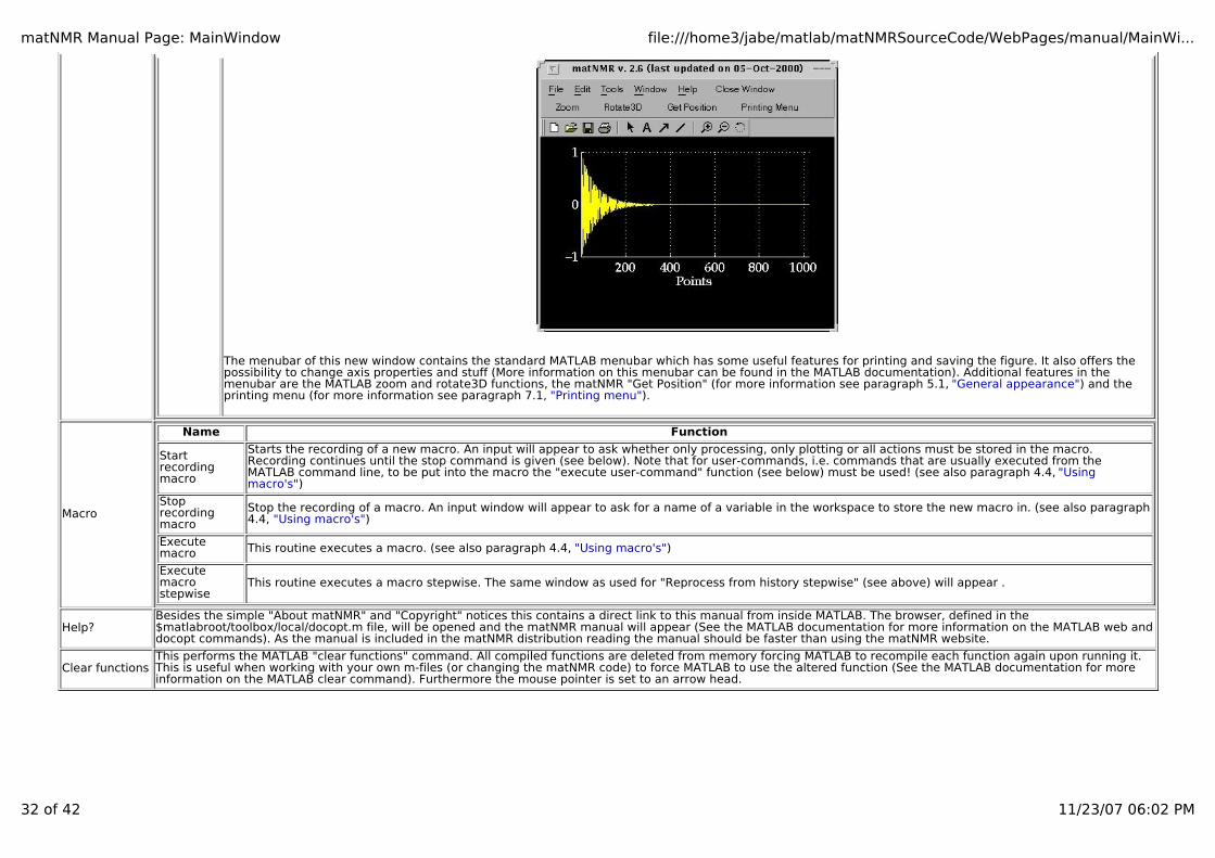
matNMR Manual Page: MainWindow file:///home3/jabe/matlab/matNMRSourceCode/WebPages/manual/MainWi...
32 of 42 11/23/07 06:02 PM
The menubar of this new window contains the standard MATLAB menubar which has some useful features for printing and saving the figure. It also offers thepossibility to change axis properties and stuff (More information on this menubar can be found in the MATLAB documentation). Additional features in themenubar are the MATLAB zoom and rotate3D functions, the matNMR "Get Position" (for more information see paragraph 5.1, "General appearance") and theprinting menu (for more information see paragraph 7.1, "Printing menu").
Macro
Name Function
Start recording macro
Starts the recording of a new macro. An input will appear to ask whether only processing, only plotting or all actions must be stored in the macro.Recording continues until the stop command is given (see below). Note that for user-commands, i.e. commands that are usually executed from theMATLAB command line, to be put into the macro the "execute user-command" function (see below) must be used! (see also paragraph 4.4, "Using macro's")
Stop recording macro
Stop the recording of a macro. An input window will appear to ask for a name of a variable in the workspace to store the new macro in. (see also paragraph4.4, "Using macro's")
Execute macro This routine executes a macro. (see also paragraph 4.4, "Using macro's")
Execute macro stepwise
This routine executes a macro stepwise. The same window as used for "Reprocess from history stepwise" (see above) will appear .
Help?Besides the simple "About matNMR" and "Copyright" notices this contains a direct link to this manual from inside MATLAB. The browser, defined in the$matlabroot/toolbox/local/docopt.m file, will be opened and the matNMR manual will appear (See the MATLAB documentation for more information on the MATLAB web anddocopt commands). As the manual is included in the matNMR distribution reading the manual should be faster than using the matNMR website.
Clear functionsThis performs the MATLAB "clear functions" command. All compiled functions are deleted from memory forcing MATLAB to recompile each function again upon running it.This is useful when working with your own m-files (or changing the matNMR code) to force MATLAB to use the altered function (See the MATLAB documentation for moreinformation on the MATLAB clear command). Furthermore the mouse pointer is set to an arrow head.
matNMR Manual Page: MainWindow file:///home3/jabe/matlab/matNMRSourceCode/WebPages/manual/MainWi...
33 of 42 11/23/07 06:02 PM
5.7 Fitting of half-integer quadrupolar tensors from MAS spectra
5.7.1 General appearance
MatNMR offers a fitting routine for quadrupolar tensors from MAS spectra which can be accessed from the "1D Processing" entry in the menubar. The following figure window will appear:
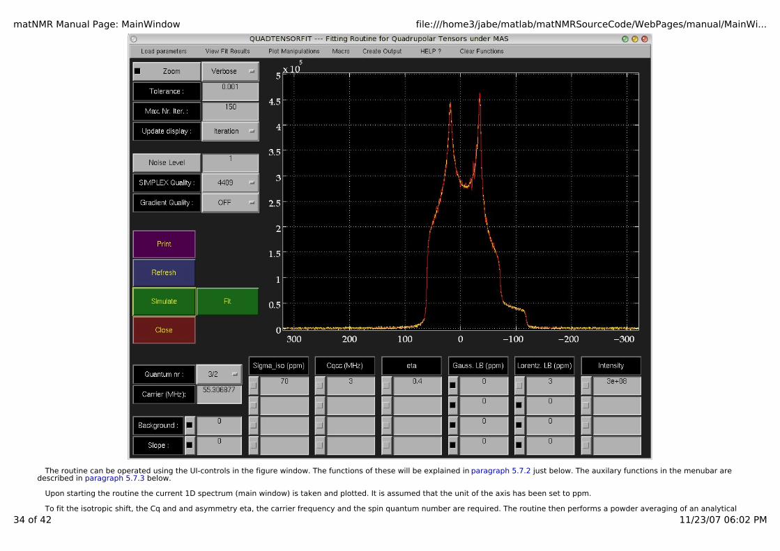
matNMR Manual Page: MainWindow file:///home3/jabe/matlab/matNMRSourceCode/WebPages/manual/MainWi...
34 of 42 11/23/07 06:02 PM
The routine can be operated using the UI-controls in the figure window. The functions of these will be explained in paragraph 5.7.2 just below. The auxilary functions in the menubar aredescribed in paragraph 5.7.3 below.
Upon starting the routine the current 1D spectrum (main window) is taken and plotted. It is assumed that the unit of the axis has been set to ppm.
To fit the isotropic shift, the Cq and and asymmetry eta, the carrier frequency and the spin quantum number are required. The routine then performs a powder averaging of an analytical
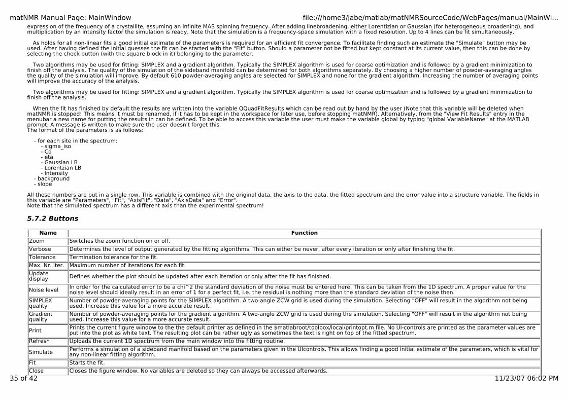
matNMR Manual Page: MainWindow file:///home3/jabe/matlab/matNMRSourceCode/WebPages/manual/MainWi...
35 of 42 11/23/07 06:02 PM
expression of the frequency of a crystallite, assuming an infinite MAS spinning frequency. After adding linebroadening, either Lorentizian or Gaussian (for heterogeneous broadening), andmultiplication by an intensity factor the simulation is ready. Note that the simulation is a frequency-space simulation with a fixed resolution. Up to 4 lines can be fit simultaneously.
As holds for all non-linear fits a good initial estimate of the parameters is required for an efficient fit convergence. To facilitate finding such an estimate the "Simulate" button may beused. After having defined the initial guesses the fit can be started with the "Fit" button. Should a parameter not be fitted but kept constant at its current value, then this can be done byselecting the check button (with the square block in it) belonging to the parameter.
Two algorithms may be used for fitting: SIMPLEX and a gradient algorithm. Typically the SIMPLEX algorithm is used for coarse optimization and is followed by a gradient minimization tofinish off the analysis. The quality of the simulation of the sideband manifold can be determined for both algorithms separately. By choosing a higher number of powder-averaging anglesthe quality of the simulation will improve. By default 610 powder-averaging angles are selected for SIMPLEX and none for the gradient algorithm. Increasing the number of averaging pointswill improve the accuracy of the analysis.
Two algorithms may be used for fitting: SIMPLEX and a gradient algorithm. Typically the SIMPLEX algorithm is used for coarse optimization and is followed by a gradient minimization tofinish off the analysis.
When the fit has finished by default the results are written into the variable QQuadFitResults which can be read out by hand by the user (Note that this variable will be deleted whenmatNMR is stopped! This means it must be renamed, if it has to be kept in the workspace for later use, before stopping matNMR). Alternatively, from the "View Fit Results" entry in themenubar a new name for putting the results in can be defined. To be able to access this variable the user must make the variable global by typing "global VariableName" at the MATLABprompt. A message is written to make sure the user doesn't forget this.The format of the parameters is as follows:
- for each site in the spectrum: - sigma_iso - Cq - eta - Gaussian LB - Lorentzian LB - Intensity - background - slope
All these numbers are put in a single row. This variable is combined with the original data, the axis to the data, the fitted spectrum and the error value into a structure variable. The fields inthis variable are "Parameters", "Fit", "AxisFit", "Data", "AxisData" and "Error".Note that the simulated spectrum has a different axis than the experimental spectrum!
5.7.2 Buttons
Name Function
Zoom Switches the zoom function on or off.
Verbose Determines the level of output generated by the fitting algorithms. This can either be never, after every iteration or only after finishing the fit.
Tolerance Termination tolerance for the fit.
Max. Nr. Iter. Maximum number of iterations for each fit.
Update display Defines whether the plot should be updated after each iteration or only after the fit has finished.
Noise level In order for the calculated error to be a chi^2 the standard deviation of the noise must be entered here. This can be taken from the 1D spectrum. A proper value for thenoise level should ideally result in an error of 1 for a perfect fit, i.e. the residual is nothing more than the standard deviation of the noise then.
SIMPLEX quality
Number of powder-averaging points for the SIMPLEX algorithm. A two-angle ZCW grid is used during the simulation. Selecting "OFF" will result in the algorithm not beingused. Increase this value for a more accurate result.
Gradient quality
Number of powder-averaging points for the gradient algorithm. A two-angle ZCW grid is used during the simulation. Selecting "OFF" will result in the algorithm not beingused. Increase this value for a more accurate result.
Print Prints the current figure window to the the default printer as defined in the $matlabroot/toolbox/local/printopt.m file. No UI-controls are printed as the parameter values areput into the plot as white text. The resulting plot can be rather ugly as sometimes the text is right on top of the fitted spectrum.
Refresh Uploads the current 1D spectrum from the main window into the fitting routine.
Simulate Performs a simulation of a sideband manifold based on the parameters given in the UIcontrols. This allows finding a good initial estimate of the parameters, which is vital forany non-linear fitting algorithm.
Fit Starts the fit.
Close Closes the figure window. No variables are deleted so they can always be accessed afterwards.
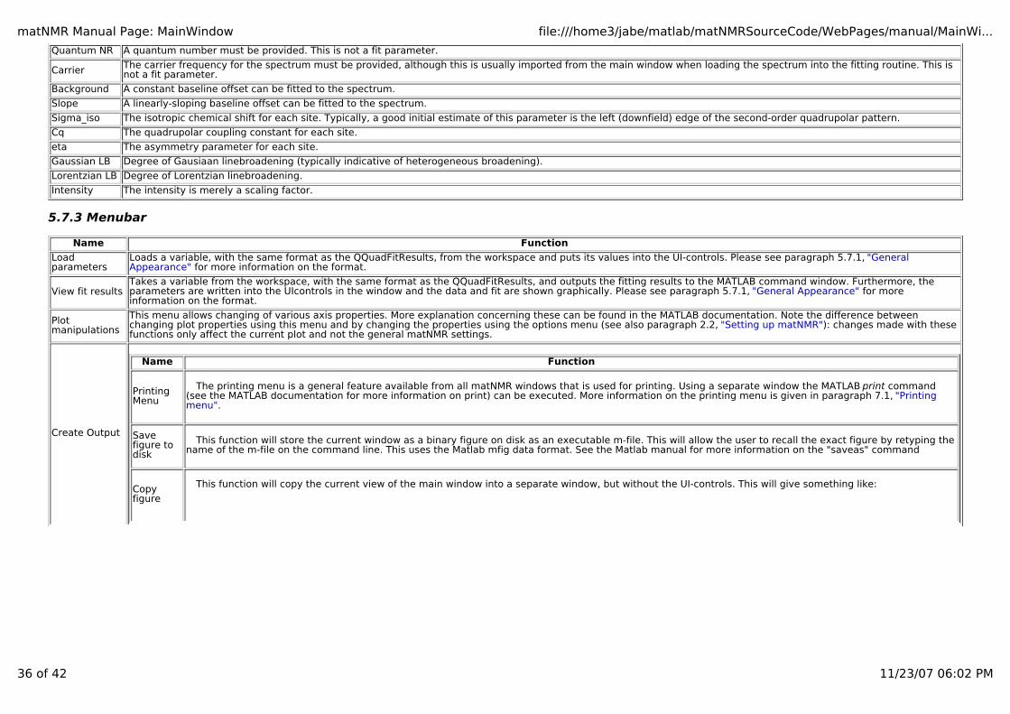
matNMR Manual Page: MainWindow file:///home3/jabe/matlab/matNMRSourceCode/WebPages/manual/MainWi...
36 of 42 11/23/07 06:02 PM
Quantum NR A quantum number must be provided. This is not a fit parameter.
Carrier The carrier frequency for the spectrum must be provided, although this is usually imported from the main window when loading the spectrum into the fitting routine. This isnot a fit parameter.
Background A constant baseline offset can be fitted to the spectrum.
Slope A linearly-sloping baseline offset can be fitted to the spectrum.
Sigma_iso The isotropic chemical shift for each site. Typically, a good initial estimate of this parameter is the left (downfield) edge of the second-order quadrupolar pattern.
Cq The quadrupolar coupling constant for each site.
eta The asymmetry parameter for each site.
Gaussian LB Degree of Gausiaan linebroadening (typically indicative of heterogeneous broadening).
Lorentzian LB Degree of Lorentzian linebroadening.
Intensity The intensity is merely a scaling factor.
5.7.3 Menubar
Name Function
Load parameters
Loads a variable, with the same format as the QQuadFitResults, from the workspace and puts its values into the UI-controls. Please see paragraph 5.7.1, "General Appearance" for more information on the format.
View fit resultsTakes a variable from the workspace, with the same format as the QQuadFitResults, and outputs the fitting results to the MATLAB command window. Furthermore, theparameters are written into the UIcontrols in the window and the data and fit are shown graphically. Please see paragraph 5.7.1, "General Appearance" for more information on the format.
Plot manipulations
This menu allows changing of various axis properties. More explanation concerning these can be found in the MATLAB documentation. Note the difference betweenchanging plot properties using this menu and by changing the properties using the options menu (see also paragraph 2.2, "Setting up matNMR"): changes made with thesefunctions only affect the current plot and not the general matNMR settings.
Create Output
Name Function
Printing Menu
The printing menu is a general feature available from all matNMR windows that is used for printing. Using a separate window the MATLAB print command (see the MATLAB documentation for more information on print) can be executed. More information on the printing menu is given in paragraph 7.1, "Printing menu".
Save figure to disk
This function will store the current window as a binary figure on disk as an executable m-file. This will allow the user to recall the exact figure by retyping thename of the m-file on the command line. This uses the Matlab mfig data format. See the Matlab manual for more information on the "saveas" command
Copy figure
This function will copy the current view of the main window into a separate window, but without the UI-controls. This will give something like:

matNMR Manual Page: MainWindow file:///home3/jabe/matlab/matNMRSourceCode/WebPages/manual/MainWi...
37 of 42 11/23/07 06:02 PM
The menubar of this new window contains the standard MATLAB menubar which has some useful features for printing and saving the figure. It also offers thepossibility to change axis properties and stuff (More information on this menubar can be found in the MATLAB documentation). Additional features in themenubar are the MATLAB zoom and rotate3D functions, the matNMR "Get Position" (for more information see paragraph 5.1, "General appearance") and theprinting menu (for more information see paragraph 7.1, "Printing menu").
Macro
Name Function
Start recording macro
Starts the recording of a new macro. An input will appear to ask whether only processing, only plotting or all actions must be stored in the macro.Recording continues until the stop command is given (see below). Note that for user-commands, i.e. commands that are usually executed from theMATLAB command line, to be put into the macro the "execute user-command" function (see below) must be used! (see also paragraph 4.4, "Using macro's")
Stop recording macro
Stop the recording of a macro. An input window will appear to ask for a name of a variable in the workspace to store the new macro in. (see also paragraph4.4, "Using macro's")
Execute macro This routine executes a macro. (see also paragraph 4.4, "Using macro's")
Execute macro stepwise
This routine executes a macro stepwise. The same window as used for "Reprocess from history stepwise" (see above) will appear .
Help?Besides the simple "About matNMR" and "Copyright" notices this contains a direct link to this manual from inside MATLAB. The browser, defined in the$matlabroot/toolbox/local/docopt.m file, will be opened and the matNMR manual will appear (See the MATLAB documentation for more information on the MATLAB web anddocopt commands). As the manual is included in the matNMR distribution reading the manual should be faster than using the matNMR website.
Clear functionsThis performs the MATLAB "clear functions" command. All compiled functions are deleted from memory forcing MATLAB to recompile each function again upon running it.This is useful when working with your own m-files (or changing the matNMR code) to force MATLAB to use the altered function (See the MATLAB documentation for moreinformation on the MATLAB clear command). Furthermore the mouse pointer is set to an arrow head.

matNMR Manual Page: MainWindow file:///home3/jabe/matlab/matNMRSourceCode/WebPages/manual/MainWi...
38 of 42 11/23/07 06:02 PM
5.8 Relaxation curve fitting
5.8.1 General appearance
MatNMR offers a basic multi-exponential fitting routine from the "1D Processing" entry in the menubar. The following figure window will appear:
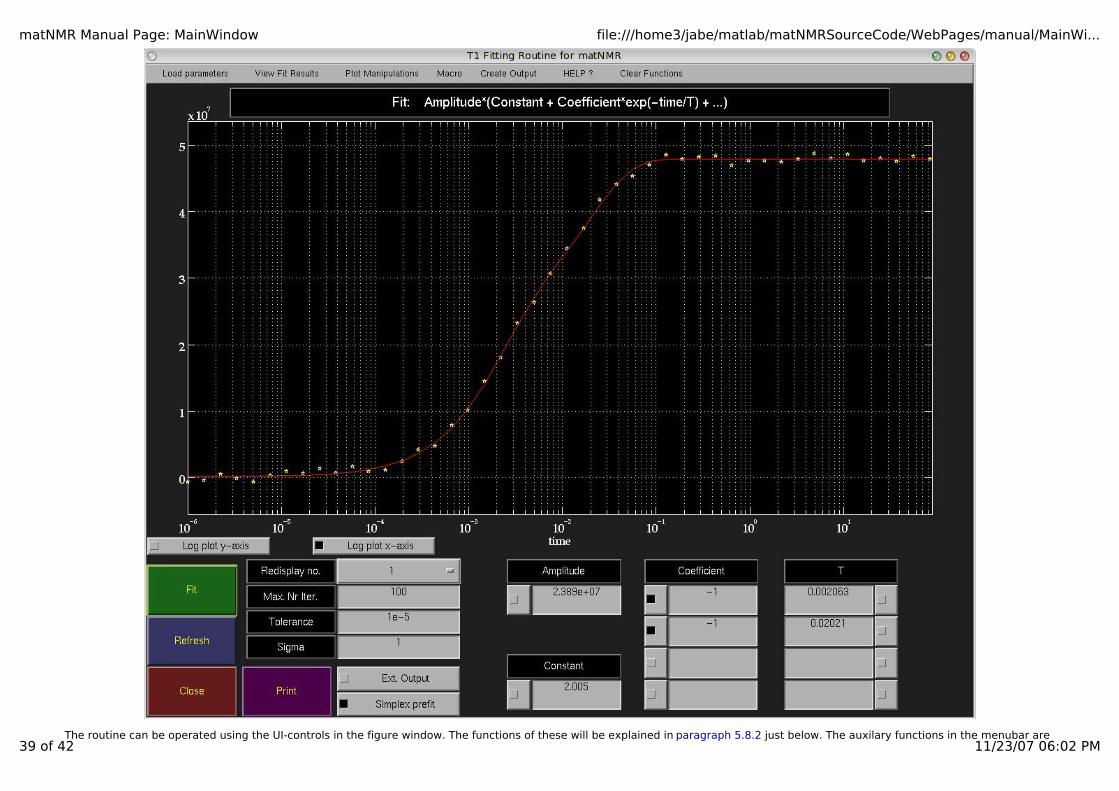
matNMR Manual Page: MainWindow file:///home3/jabe/matlab/matNMRSourceCode/WebPages/manual/MainWi...
39 of 42 11/23/07 06:02 PMThe routine can be operated using the UI-controls in the figure window. The functions of these will be explained in paragraph 5.8.2 just below. The auxilary functions in the menubar are
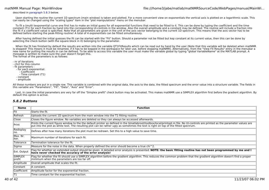
matNMR Manual Page: MainWindow file:///home3/jabe/matlab/matNMRSourceCode/WebPages/manual/MainWi...
40 of 42 11/23/07 06:02 PM
described in paragraph 5.8.3 below.
Upon starting the routine the current 1D spectrum (main window) is taken and plotted. For a more convenient view on exponentials the vertical axis is plotted on a logarithmic scale. Thiscan easily be changed using the "scaling types" item in the "plot manipulations" menu on the menubar.
To fit a (multi-)exponential curve one first has to make an initial guess for all exponential functions that need to be fitted to it. This can be done by typing the coefficient and the timeconstant (T1) for each fraction by hand into the corresponding UI-controls in the window. Also the overall amplitude and a constant may be defined. The routine will include a fraction intothe fit if a coefficient value is specified. Note that all parameters are given in the unit of the axis vector belonging to the current 1D spectrum. This means that the axis vector has to bedefined before starting the peak-fitting routine! A total of 4 exponentials can be fitted simultaneouly.
After having defined the initial guesses the fit can be started with the "Fit" button. Should a parameter not be fitted but kep constant at its current value, then this can be done byselecting the check button (with the square block in it) belonging to the parameter.
When the fit has finished by default the results are written into the variable QT1FitResults which can be read out by hand by the user (Note that this variable will be deleted when matNMRis stopped! This means it must be renamed, if it has to be kepped in the workspace for later use, before stopping matNMR). Alternatively, from the "View Fit Results" entry in the menubar anew name for putting the results in can be defined. To be able to access this variable the user must make the variable global by typing "global VariableName" at the MATLAB prompt. Amessage is written to make sure the user doesn't forget this.The format of the parameters is as follows:
- nr of iterations- chi2 for this column- fit parameters : - for each exponential: - Coefficient - Time constant (T1) - constant - amplitude
All these numbers are put in a single row. This variable is combined with the original data, the axis to the data, the fitted spectrum and the error value into a structure variable. The fields inthis variable are "Parameters", "Fit", "Data", "Axis" and "Error".
Last, in case the initial parameters are very far off the "Simplex prefit" check button may be activated. This makes matNMR use a SIMPLEX algorithm first before the gradient algorithm. Bydefault this option is active.
5.8.2 Buttons
Name Function
Fit Starts the fit.
Refresh Uploads the current 1D spectrum from the main window into the T1-fitting routine.
Close Closes the figure window. No variables are deleted so they can always be accessed afterwards.
Print Prints the current figure window to the the default printer as defined in the $matlabroot/toolbox/local/printopt.m file. No UI-controls are printed as the parameter values areput into the plot as white text. The resulting plot can be rather ugly as sometimes the text is right on top of the fitted spectrum.
Redisplay no. Defines after how many iterations the plot must be redrawn. Set this to a high value to save time.
Max. Nr. Iter. Maximum number of iterations for each fit.
Tolerance Termination tolerance for the fit.
Sigma Measure for the noise in the data. When properly defined the error should become a true chi^2.
Ext. Output Flag for whether an extended output should be given. A detailed error analysis is presented. NOTE: the basic fitting routine has not been programmed by me and Ihave never checked the accuracy of the error analysis!
SIMPLEX prefit
Flag for whether the fit should use a SIMPLEX algorithm before the gradient algorithm. This reduces the common problem that the gradient algorithm doesn't find a properminimum when the parameters are too far off.
Amplitude Overall amplitude that scales the fit.
Constant A constant.
Coefficient Amplitude factor for the exponential fraction.
T1 Time constant for the exponential fraction.
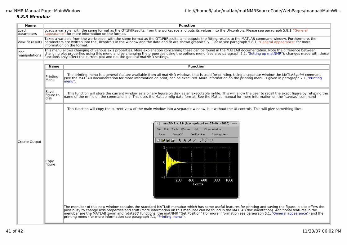
matNMR Manual Page: MainWindow file:///home3/jabe/matlab/matNMRSourceCode/WebPages/manual/MainWi...
41 of 42 11/23/07 06:02 PM
5.8.3 Menubar
Name Function
Load parameters
Loads a variable, with the same format as the QT1FitResults, from the workspace and puts its values into the UI-controls. Please see paragraph 5.8.1, "General Appearance" for more information on the format.
View fit resultsTakes a variable from the workspace, with the same format as the QT1FitResults, and outputs the fitting results to the MATLAB command window. Furthermore, theparameters are written into the UIcontrols in the window and the data and fit are shown graphically. Please see paragraph 5.8.1, "General Appearance" for more information on the format.
Plot manipulations
This menu allows changing of various axis properties. More explanation concerning these can be found in the MATLAB documentation. Note the difference betweenchanging plot properties using this menu and by changing the properties using the options menu (see also paragraph 2.2, "Setting up matNMR"): changes made with thesefunctions only affect the current plot and not the general matNMR settings.
Create Output
Name Function
Printing Menu
The printing menu is a general feature available from all matNMR windows that is used for printing. Using a separate window the MATLAB print command (see the MATLAB documentation for more information on print) can be executed. More information on the printing menu is given in paragraph 7.1, "Printing menu".
Save figure to disk
This function will store the current window as a binary figure on disk as an executable m-file. This will allow the user to recall the exact figure by retyping thename of the m-file on the command line. This uses the Matlab mfig data format. See the Matlab manual for more information on the "saveas" command
Copy figure
This function will copy the current view of the main window into a separate window, but without the UI-controls. This will give something like:
The menubar of this new window contains the standard MATLAB menubar which has some useful features for printing and saving the figure. It also offers thepossibility to change axis properties and stuff (More information on this menubar can be found in the MATLAB documentation). Additional features in themenubar are the MATLAB zoom and rotate3D functions, the matNMR "Get Position" (for more information see paragraph 5.1, "General appearance") and theprinting menu (for more information see paragraph 7.1, "Printing menu").
matNMR Manual Page: MainWindow file:///home3/jabe/matlab/matNMRSourceCode/WebPages/manual/MainWi...
42 of 42 11/23/07 06:02 PM
Macro
Name Function
Start recording macro
Starts the recording of a new macro. An input will appear to ask whether only processing, only plotting or all actions must be stored in the macro.Recording continues until the stop command is given (see below). Note that for user-commands, i.e. commands that are usually executed from theMATLAB command line, to be put into the macro the "execute user-command" function (see below) must be used! (see also paragraph 4.4, "Using macro's")
Stop recording macro
Stop the recording of a macro. An input window will appear to ask for a name of a variable in the workspace to store the new macro in. (see also paragraph4.4, "Using macro's")
Execute macro This routine executes a macro. (see also paragraph 4.4, "Using macro's")
Execute macro stepwise
This routine executes a macro stepwise. The same window as used for "Reprocess from history stepwise" (see above) will appear .
Help?Besides the simple "About matNMR" and "Copyright" notices this contains a direct link to this manual from inside MATLAB. The browser, defined in the$matlabroot/toolbox/local/docopt.m file, will be opened and the matNMR manual will appear (See the MATLAB documentation for more information on the MATLAB web anddocopt commands). As the manual is included in the matNMR distribution reading the manual should be faster than using the matNMR website.
Clear functionsThis performs the MATLAB "clear functions" command. All compiled functions are deleted from memory forcing MATLAB to recompile each function again upon running it.This is useful when working with your own m-files (or changing the matNMR code) to force MATLAB to use the altered function (See the MATLAB documentation for moreinformation on the MATLAB clear command). Furthermore the mouse pointer is set to an arrow head.

matNMR Manual Page: 2D/3D viewer file:///home3/jabe/matlab/matNMRSourceCode/WebPages/manual/2D3DVi...
1 of 20 11/23/07 06:03 PM
Chapter 6 - The 2D/3D ViewerThe 2D/3D Viewer is started using the nmr2d.m script, i.e. type 'nmr2d' at the Matlab prompt to start it.
6.1 General Appearance
The general appearance of the 2D/3D Viewer window consists of two parts and is shown in the figures below:
A typical data window:
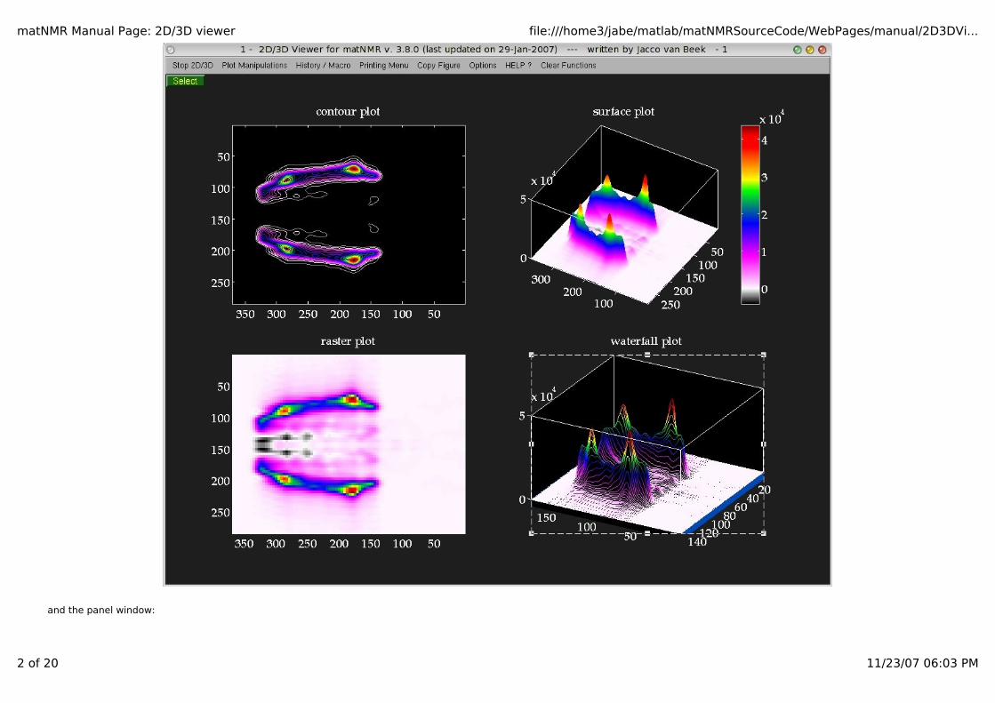
matNMR Manual Page: 2D/3D viewer file:///home3/jabe/matlab/matNMRSourceCode/WebPages/manual/2D3DVi...
2 of 20 11/23/07 06:03 PM
and the panel window:

matNMR Manual Page: 2D/3D viewer file:///home3/jabe/matlab/matNMRSourceCode/WebPages/manual/2D3DVi...
3 of 20 11/23/07 06:03 PM
The 2D/3D Viewer is a multi-window multi-plot routine: an arbitrary number of windows can be opened (simultaneously) and they can all have an arbitrary number of subplots (only limitedby the number of pre-defined subplot configurations matNMR allows). All data windows are controlled from the panel window. Any function executed from here will apply to the current axisin the current 2D/3D Viewer window. The current axis is always marked by a box around it. The current figure though is not always so clearly recognizable. In general the current figure willbe pulled in front before executing a plotting command, making it clear what the current figure window is. In general it is NOT sufficient to pull the window in front if one wants to make a figure the current figure! The preferred way of selecting a window therefore is to click on the "Select" button in the top left corner of the window, or alternatively inside the window (Not onthe menubar!).
Although this routine is multi-window multi-plot only one set of variables is kept in memory (for more information on memory usage see also paragraph 3.7, "Memory usage"). This means that only the matrix (and axis vectors etc.) belonging to the last plotted spectrum is stored. This is important to realize because it affects certain routines that use the matrix forextracting spectral intensities like Integrate, peak picking, get position, etc. These only function properly for the last plotted spectrum. And although they may not produce any errors, theresult may still be wrong! Some plot parameters are stored into the figure window and they contain some information on each specific plot in the figure:-name-axis vectors: extracting axis coordinates will work properly even when the plot does not belong to the last plotted spectrum!-processing history
Furthermore certain properties of the current figure are saved:-number of subplots-axis handles-colorbar flags for each axis-colorbar handles-zoom flag-rotate3D flag
All these parameters are stored into the userdata property of the figure (for more information on properties of graphics objects see the MATLAB documentation). Extracting this property(e.g. QTEMP= get(gcf, 'userdata')) will result in a structure variable. Users can add fields to it (in principle the userdata property is free to be manipulated in any way and can therefore beuseful for various things) but shouldn't removed the fields that matNMR has created sofar as this will produce errors. .
The functions panel window will be explained in paragraph 6.2, just below and the menubar in the data windows in paragraph 6.3, "The menubar".
6.2 The panel window
The panel window has been subdivided into the four major plot types currently supported by matNMR, contours, mesh, Stack 3D and raster plot and a tools menu. They will be explainedseparately below. Note that although the functions explained below are separated into discrete categories they can be used as general functions.
Note that all the items in the "Tools" menu can be started also from the Plotmanipulations menu in the menubar.
6.2.1 Contours

matNMR Manual Page: 2D/3D viewer file:///home3/jabe/matlab/matNMRSourceCode/WebPages/manual/2D3DVi...
4 of 20 11/23/07 06:03 PM
Button Function
Contour Popup button for selecting the type of contour plot. Currently supported are the three MATLAB contour routines contour (normal contours), contourf (filled contours) andcontour3 (contours plotted at their corresponding z-level). See the MATLAB documentation for more information on these routines.
Real Popup button for selecting whether to plot the real, the imaginary or the absolute value of a matrix.
Relative Contours
This function allows plotting relative contours, i.e. the contour levels are specified as a percentage of the maximum intensity of a matrix. The following input window willappear:
The following fields must be specified:Field Function
Name Spectrum
This must be either a name of a matrix variable in the workspace or a function generating a matrix as output. In case the variable is a matNMR structure (see alsoparagraph 3.5, "matNMR format for spectra") then the routine will extract the corresponding axis vectors (and history etc) that were saved into it. If axis vectorsare specified in this input window (see below) for Td2 and/or TD1 then these are used and not the axis vectors as saved in the structure.
Lower contour limit
Defines the lower contour limit as a percentage of the maximum intensity of the matrix.

matNMR Manual Page: 2D/3D viewer file:///home3/jabe/matlab/matNMRSourceCode/WebPages/manual/2D3DVi...
5 of 20 11/23/07 06:03 PM
Upper contour limit
Defines the upper contour limit as a percentage of the maximum intensity of the matrix.
MultiplierA number that specifies the non-linearity of the increment between contour levels. If (Multiplier = 1) then the increment between contour levels is the same for allcontour levels. If (0 < Multiplier < 1) then more contours are drawn towards the high end of the range as defined by the lower and upper limits. If (Multiplier > 1)then more contour levels are drawn towards the lower end of the range.
Number of contours
The total number of contour levels in the plot. When both positive and negative contours are asked for then a vector of two numbers may be given to denotedifferent numbers of contours for positive and negative intensities. If only one number is specified then both positive and negative intensities have the samenumber of contours.
Type of contours
This determines how the contour levels will be calculated. This can either be a) positive contours (i.e. relative to the positive maximum), (b) negative contours(i.e. relative to the negative maximum), c) both positive and negative contours (relative to the respective positive and negative maxima), d) both positive andnegative contours but relative to the positive maximum or e) both positive and negative contours but relative to the negative maximum of the spectrum. Notethat for the last three options the number of contours is doubled (if a contour level is set at 0, the number of contours is doubled minus 1). A special colormap willbe generated when printing both positive and negative contours.
Vector for TD2-axis
A variable in the workspace corresponding to the axis vector for this dimension. Leaving this empty will give an axis in points unless the "Name Spectrum" is amatNMR structure (see "Name Spectrum"). Specifying an axis vector will overrule any axis vector saved in the variable structure.
Vector for TD1-axis
A variable in the workspace corresponding to the axis vector for this dimension. Leaving this empty will give an axis in points unless the "Name Spectrum" is amatNMR structure (see "Name Spectrum"). Specifying an axis vector will overrule any axis vector saved in the variable structure.
LinespecLeaving this empty will plot the contours as a MATLAB patch (for more information on this see the MATLAB documentation), meaning it will use a colormap.Specifying the linespec causes MATLAB to plot the contours as line plots. See the MATLAB documentation for more information on colormaps and linespecproperties.
Plotting Macro Allows for a plotting macro to be executed immediately after the plot is made, in order to reduce rendering time. See also paragraph 4.4, "Using macro's".
Absolute Contours
This function allows plotting absolute contours, i.e. the contour levels are specified directly by the user. The following input window will appear:
The following fields must be specified:Field Function
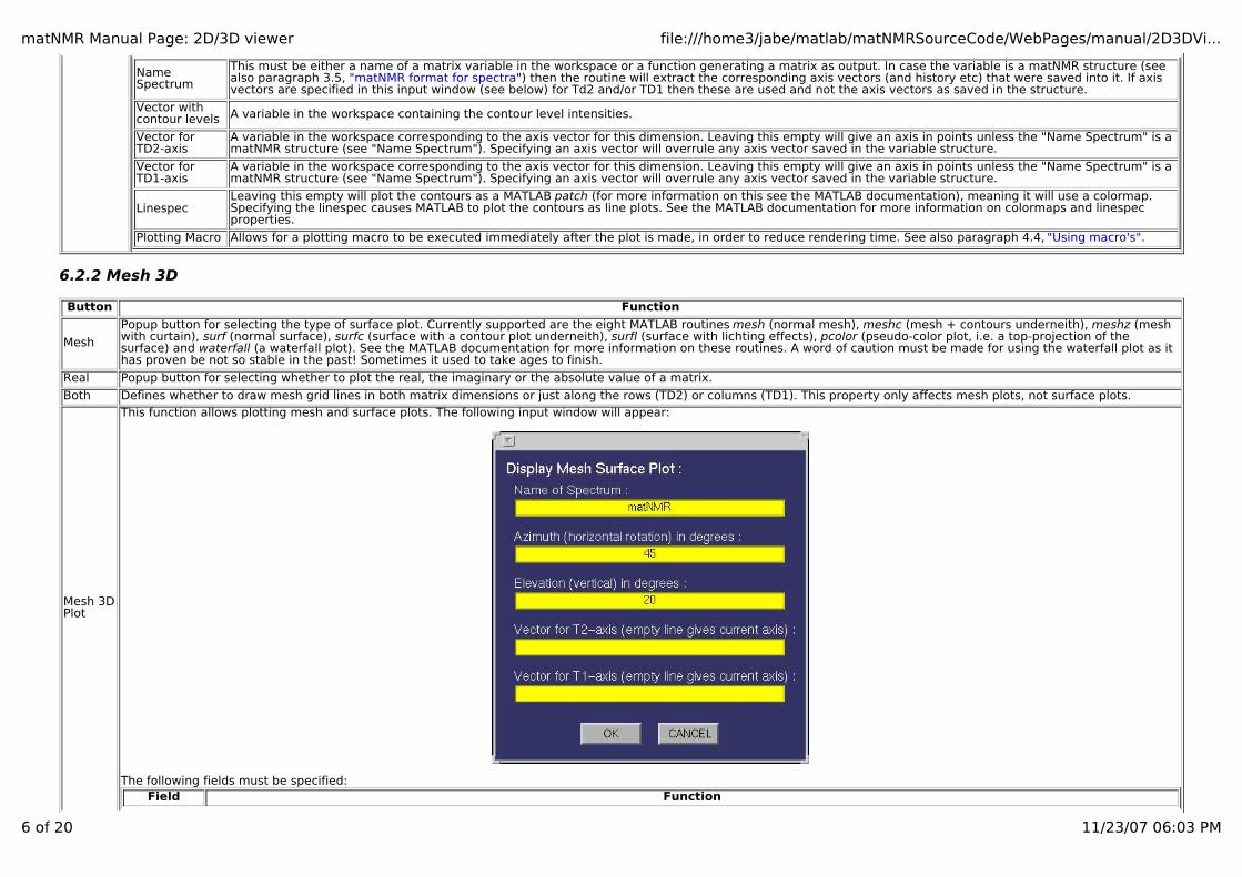
matNMR Manual Page: 2D/3D viewer file:///home3/jabe/matlab/matNMRSourceCode/WebPages/manual/2D3DVi...
6 of 20 11/23/07 06:03 PM
Name Spectrum
This must be either a name of a matrix variable in the workspace or a function generating a matrix as output. In case the variable is a matNMR structure (seealso paragraph 3.5, "matNMR format for spectra") then the routine will extract the corresponding axis vectors (and history etc) that were saved into it. If axisvectors are specified in this input window (see below) for Td2 and/or TD1 then these are used and not the axis vectors as saved in the structure.
Vector with contour levels A variable in the workspace containing the contour level intensities.
Vector for TD2-axis
A variable in the workspace corresponding to the axis vector for this dimension. Leaving this empty will give an axis in points unless the "Name Spectrum" is amatNMR structure (see "Name Spectrum"). Specifying an axis vector will overrule any axis vector saved in the variable structure.
Vector for TD1-axis
A variable in the workspace corresponding to the axis vector for this dimension. Leaving this empty will give an axis in points unless the "Name Spectrum" is amatNMR structure (see "Name Spectrum"). Specifying an axis vector will overrule any axis vector saved in the variable structure.
LinespecLeaving this empty will plot the contours as a MATLAB patch (for more information on this see the MATLAB documentation), meaning it will use a colormap.Specifying the linespec causes MATLAB to plot the contours as line plots. See the MATLAB documentation for more information on colormaps and linespecproperties.
Plotting Macro Allows for a plotting macro to be executed immediately after the plot is made, in order to reduce rendering time. See also paragraph 4.4, "Using macro's".
6.2.2 Mesh 3D
Button Function
Mesh
Popup button for selecting the type of surface plot. Currently supported are the eight MATLAB routines mesh (normal mesh), meshc (mesh + contours underneith), meshz (mesh with curtain), surf (normal surface), surfc (surface with a contour plot underneith), surfl (surface with lichting effects), pcolor (pseudo-color plot, i.e. a top-projection of thesurface) and waterfall (a waterfall plot). See the MATLAB documentation for more information on these routines. A word of caution must be made for using the waterfall plot as ithas proven be not so stable in the past! Sometimes it used to take ages to finish.
Real Popup button for selecting whether to plot the real, the imaginary or the absolute value of a matrix.
Both Defines whether to draw mesh grid lines in both matrix dimensions or just along the rows (TD2) or columns (TD1). This property only affects mesh plots, not surface plots.
Mesh 3D Plot
This function allows plotting mesh and surface plots. The following input window will appear:
The following fields must be specified:Field Function
matNMR Manual Page: 2D/3D viewer file:///home3/jabe/matlab/matNMRSourceCode/WebPages/manual/2D3DVi...
7 of 20 11/23/07 06:03 PM
Name Spectrum
This must be either a name of a matrix variable in the workspace or a function generating a matrix as output. In case the variable is a matNMR structure (see alsoparagraph 3.5, "matNMR format for spectra") then the routine will extract the corresponding axis vectors (and history etc) that were saved into it. If axis vectorsare specified in this input window (see below) for Td2 and/or TD1 then these are used and not the axis vectors as saved in the structure.
Azimuthal Defines the azimuth angle or better the horizontal rotation angle for the resulting view (see MATLAB documentation for more information on view). The view canalways be changed by using the Rotate3D function in the Tools section (described below).
Elevation Defines the elevation angle or better the vertical rotation angle for the resulting view (see MATLAB documentation for more information on view). The view canalways be changed by using the Rotate3D function in the Tools section (described below).
Vector for TD2-axis
A variable in the workspace corresponding to the axis vector for this dimension. Leaving this empty will give an axis in points unless the "Name Spectrum" is amatNMR structure (see "Name Spectrum"). Specifying an axis vector will overrule any axis vector saved in the variable structure.
Vector for TD1-axis
A variable in the workspace corresponding to the axis vector for this dimension. Leaving this empty will give an axis in points unless the "Name Spectrum" is amatNMR structure (see "Name Spectrum"). Specifying an axis vector will overrule any axis vector saved in the variable structure.
Plotting Macro Allows for a plotting macro to be executed immediately after the plot is made, in order to reduce rendering time. See also paragraph 4.4, "Using macro's".
6.2.3 Stack 3D
3D Stack plots are plots in which, along one dimension of the matrix, the lines are stacked such that a spatial view is obtained. This can be very useful for watching decays etc.
Button Function
Lower z-limit Defines the lower zlimit for the plot. If not defined before plotting a new matrix then matNMR will set it to the default axis settings after plotting the matrix.
Upper z-limit Defines the upper zlimit for the plot. If not defined before plotting a new matrix then matNMR will set it to the default axis settings after plotting the matrix.
Real Popup button for selecting whether to plot the real, the imaginary or the absolute value of a matrix.
Y-dir default Defines the default axis direction for the plot. Usually this is set to right-to-left for NMR spectra but this is not necessarily what is needed for a plot.
Stack 3D This function allows plotting 3D stack plots. The following input window will appear:
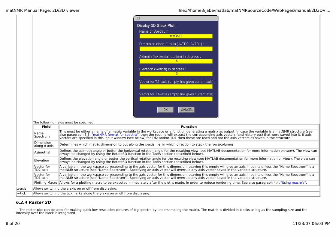
matNMR Manual Page: 2D/3D viewer file:///home3/jabe/matlab/matNMRSourceCode/WebPages/manual/2D3DVi...
8 of 20 11/23/07 06:03 PM
The following fields must be specified:Field Function
Name Spectrum
This must be either a name of a matrix variable in the workspace or a function generating a matrix as output. In case the variable is a matNMR structure (seealso paragraph 3.5, "matNMR format for spectra") then the routine will extract the corresponding axis vectors (and history etc) that were saved into it. If axisvectors are specified in this input window (see below) for Td2 and/or TD1 then these are used and not the axis vectors as saved in the structure.
Dimension along x-axis Determines which matrix dimension to put along the x-axis, i.e. in which direction to stack the rows/columns.
Azimuthal Defines the azimuth angle or better the horizontal rotation angle for the resulting view (see MATLAB documentation for more information on view). The view canalways be changed by using the Rotate3D function in the Tools section (described below).
Elevation Defines the elevation angle or better the vertical rotation angle for the resulting view (see MATLAB documentation for more information on view). The view canalways be changed by using the Rotate3D function in the Tools section (described below).
Vector for TD2-axis
A variable in the workspace corresponding to the axis vector for this dimension. Leaving this empty will give an axis in points unless the "Name Spectrum" is amatNMR structure (see "Name Spectrum"). Specifying an axis vector will overrule any axis vector saved in the variable structure.
Vector for TD1-axis
A variable in the workspace corresponding to the axis vector for this dimension. Leaving this empty will give an axis in points unless the "Name Spectrum" is amatNMR structure (see "Name Spectrum"). Specifying an axis vector will overrule any axis vector saved in the variable structure.
Plotting Macro Allows for a plotting macro to be executed immediately after the plot is made, in order to reduce rendering time. See also paragraph 4.4, "Using macro's".
z-axis Allows switching the z-axis on or off from displaying.
y-tick Allows switching the tickmarks along the y-axis on or off from displaying.
6.2.4 Raster 2D
The raster plot can be used for making quick low-resolution pictures of big spectra by undersampling the matrix. The matrix is divided in blocks as big as the sampling size and theintensity over the block is integrated.
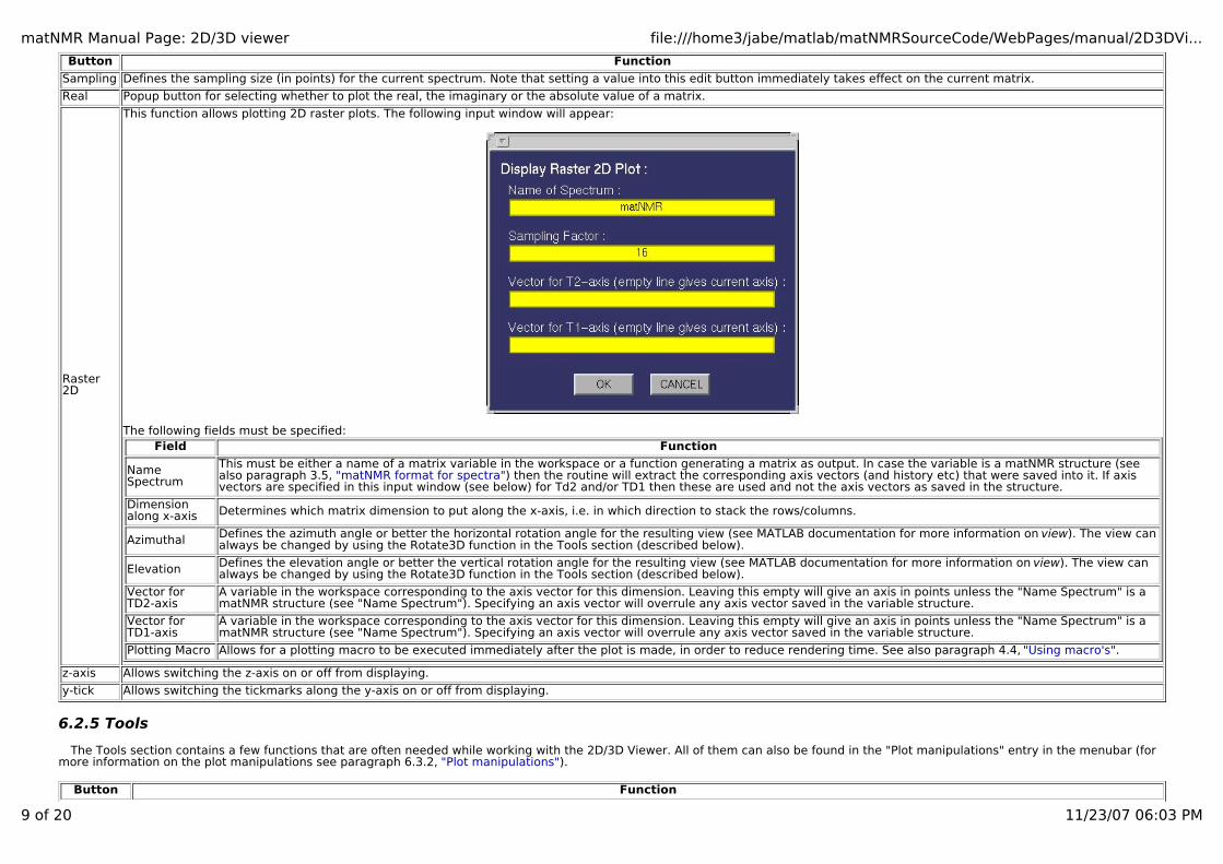
matNMR Manual Page: 2D/3D viewer file:///home3/jabe/matlab/matNMRSourceCode/WebPages/manual/2D3DVi...
9 of 20 11/23/07 06:03 PM
Button Function
Sampling Defines the sampling size (in points) for the current spectrum. Note that setting a value into this edit button immediately takes effect on the current matrix.
Real Popup button for selecting whether to plot the real, the imaginary or the absolute value of a matrix.
Raster 2D
This function allows plotting 2D raster plots. The following input window will appear:
The following fields must be specified:Field Function
Name Spectrum
This must be either a name of a matrix variable in the workspace or a function generating a matrix as output. In case the variable is a matNMR structure (seealso paragraph 3.5, "matNMR format for spectra") then the routine will extract the corresponding axis vectors (and history etc) that were saved into it. If axisvectors are specified in this input window (see below) for Td2 and/or TD1 then these are used and not the axis vectors as saved in the structure.
Dimension along x-axis Determines which matrix dimension to put along the x-axis, i.e. in which direction to stack the rows/columns.
Azimuthal Defines the azimuth angle or better the horizontal rotation angle for the resulting view (see MATLAB documentation for more information on view). The view canalways be changed by using the Rotate3D function in the Tools section (described below).
Elevation Defines the elevation angle or better the vertical rotation angle for the resulting view (see MATLAB documentation for more information on view). The view canalways be changed by using the Rotate3D function in the Tools section (described below).
Vector for TD2-axis
A variable in the workspace corresponding to the axis vector for this dimension. Leaving this empty will give an axis in points unless the "Name Spectrum" is amatNMR structure (see "Name Spectrum"). Specifying an axis vector will overrule any axis vector saved in the variable structure.
Vector for TD1-axis
A variable in the workspace corresponding to the axis vector for this dimension. Leaving this empty will give an axis in points unless the "Name Spectrum" is amatNMR structure (see "Name Spectrum"). Specifying an axis vector will overrule any axis vector saved in the variable structure.
Plotting Macro Allows for a plotting macro to be executed immediately after the plot is made, in order to reduce rendering time. See also paragraph 4.4, "Using macro's".
z-axis Allows switching the z-axis on or off from displaying.
y-tick Allows switching the tickmarks along the y-axis on or off from displaying.
6.2.5 Tools
The Tools section contains a few functions that are often needed while working with the 2D/3D Viewer. All of them can also be found in the "Plot manipulations" entry in the menubar (formore information on the plot manipulations see paragraph 6.3.2, "Plot manipulations").
Button Function
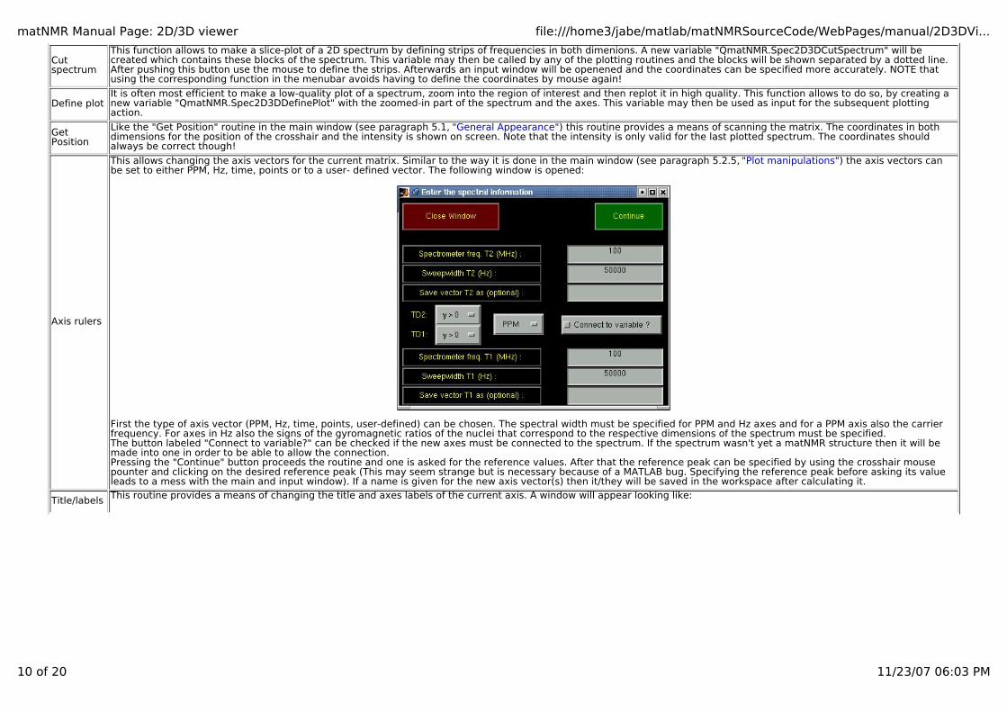
matNMR Manual Page: 2D/3D viewer file:///home3/jabe/matlab/matNMRSourceCode/WebPages/manual/2D3DVi...
10 of 20 11/23/07 06:03 PM
Cut spectrum
This function allows to make a slice-plot of a 2D spectrum by defining strips of frequencies in both dimenions. A new variable "QmatNMR.Spec2D3DCutSpectrum" will becreated which contains these blocks of the spectrum. This variable may then be called by any of the plotting routines and the blocks will be shown separated by a dotted line.After pushing this button use the mouse to define the strips. Afterwards an input window will be openened and the coordinates can be specified more accurately. NOTE thatusing the corresponding function in the menubar avoids having to define the coordinates by mouse again!
Define plotIt is often most efficient to make a low-quality plot of a spectrum, zoom into the region of interest and then replot it in high quality. This function allows to do so, by creating anew variable "QmatNMR.Spec2D3DDefinePlot" with the zoomed-in part of the spectrum and the axes. This variable may then be used as input for the subsequent plottingaction.
Get Position
Like the "Get Position" routine in the main window (see paragraph 5.1, "General Appearance") this routine provides a means of scanning the matrix. The coordinates in bothdimensions for the position of the crosshair and the intensity is shown on screen. Note that the intensity is only valid for the last plotted spectrum. The coordinates shouldalways be correct though!
Axis rulers
This allows changing the axis vectors for the current matrix. Similar to the way it is done in the main window (see paragraph 5.2.5, "Plot manipulations") the axis vectors can be set to either PPM, Hz, time, points or to a user- defined vector. The following window is opened:
First the type of axis vector (PPM, Hz, time, points, user-defined) can be chosen. The spectral width must be specified for PPM and Hz axes and for a PPM axis also the carrierfrequency. For axes in Hz also the signs of the gyromagnetic ratios of the nuclei that correspond to the respective dimensions of the spectrum must be specified.The button labeled "Connect to variable?" can be checked if the new axes must be connected to the spectrum. If the spectrum wasn't yet a matNMR structure then it will bemade into one in order to be able to allow the connection.Pressing the "Continue" button proceeds the routine and one is asked for the reference values. After that the reference peak can be specified by using the crosshair mousepounter and clicking on the desired reference peak (This may seem strange but is necessary because of a MATLAB bug. Specifying the reference peak before asking its valueleads to a mess with the main and input window). If a name is given for the new axis vector(s) then it/they will be saved in the workspace after calculating it.
Title/labels This routine provides a means of changing the title and axes labels of the current axis. A window will appear looking like:
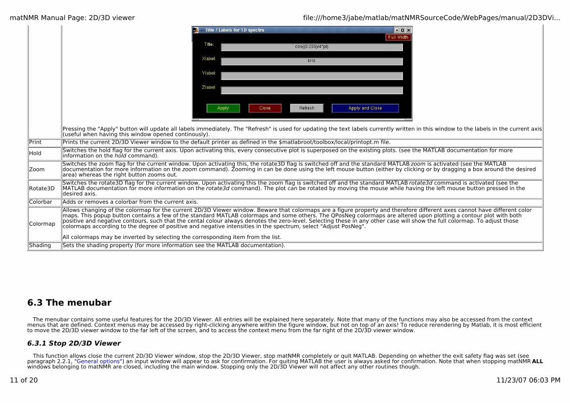
matNMR Manual Page: 2D/3D viewer file:///home3/jabe/matlab/matNMRSourceCode/WebPages/manual/2D3DVi...
11 of 20 11/23/07 06:03 PM
Pressing the "Apply" button will update all labels immediately. The "Refresh" is used for updating the text labels currently written in this window to the labels in the current axis(useful when having this window opened continously).
Print Prints the current 2D/3D Viewer window to the default printer as defined in the $matlabroot/toolbox/local/printopt.m file.
Hold Switches the hold flag for the current axis. Upon activating this, every consecutive plot is superposed on the existing plots. (see the MATLAB documentation for moreinformation on the hold command).
ZoomSwitches the zoom flag for the current window. Upon activating this, the rotate3D flag is switched off and the standard MATLAB zoom is activated (see the MATLABdocumentation for more information on the zoom command). Zooming in can be done using the left mouse button (either by clicking or by dragging a box around the desiredarea) whereas the right button zooms out.
Rotate3DSwitches the rotate3D flag for the current window. Upon activating this the zoom flag is switched off and the standard MATLAB rotate3d command is activated (see theMATLAB documentation for more information on the rotate3d command). The plot can be rotated by moving the mouse while having the left mouse button pressed in thedesired axis.
Colorbar Adds or removes a colorbar from the current axis.
Colormap
Allows changing of the colormap for the current 2D/3D Viewer window. Beware that colormaps are a figure property and therefore different axes cannot have different colormaps. This popup button contains a few of the standard MATLAB colormaps and some others. The QPosNeg colormaps are altered upon plotting a contour plot with bothpositive and negative contours, such that the cental colour always denotes the zero-level. Selecting these in any other case will show the full colormap. To adjust thosecolormaps according to the degree of positive and negative intensities in the spectrum, select "Adjust PosNeg".
All colormaps may be inverted by selecting the corresponding item from the list.
Shading Sets the shading property (for more information see the MATLAB documentation).
6.3 The menubar
The menubar contains some useful features for the 2D/3D Viewer. All entries will be explained here separately. Note that many of the functions may also be accessed from the contextmenus that are defined. Context menus may be accessed by right-clicking anywhere within the figure window, but not on top of an axis! To reduce rerendering by Matlab, it is most efficientto move the 2D/3D viewer window to the far left of the screen, and to access the context menu from the far right of the 2D/3D viewer window.
6.3.1 Stop 2D/3D Viewer
This function allows close the current 2D/3D Viewer window, stop the 2D/3D Viewer, stop matNMR completely or quit MATLAB. Depending on whether the exit safety flag was set (seeparagraph 2.2.1, "General options") an input window will appear to ask for confirmation. For quiting MATLAB the user is always asked for confirmation. Note that when stopping matNMR ALLwindows belonging to matNMR are closed, including the main window. Stopping only the 2D/3D Viewer will not affect any other routines though.
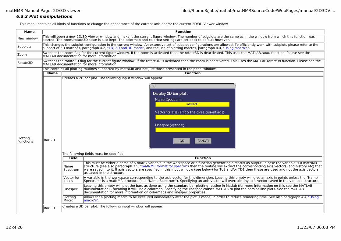
matNMR Manual Page: 2D/3D viewer file:///home3/jabe/matlab/matNMRSourceCode/WebPages/manual/2D3DVi...
12 of 20 11/23/07 06:03 PM
6.3.2 Plot manipulations
This menu contains all kinds of functions to change the appearance of the current axis and/or the current 2D/3D Viewer window.
Name Function
New window This will open a new 2D/3D Viewer window and make it the current figure window. The number of subplots are the same as in the window from which this function wasstarted. The zoom/rotate3D state is also kept. The colormap and colorbar settings are set back to default however.
Subplots This changes the subplot configuration in the current window. An extensive set of subplot configurations are allowed. To efficiently work with subplots please refer to thesupport of 3D matrices, paragraph 4.2, "1D, 2D and 3D mode", and the use of plotting macros, paragraph 4.4, "Using macro's".
Zoom Switches the zoom flag for the current figure window. If the zoom is activated then the rotate3D is deactivated. This uses the MATLAB zoom function. Please see theMATLAB documentation for more information.
Rotate3D Switches the rotate3D flag for the current figure window. If the rotate3D is activated then the zoom is deactivated. This uses the MATLAB rotate3d function. Please see theMATLAB documentation for more information.
Plotting Functions
This contains all plotting routines supported by matNMR and not just those presented in the panel window.Name Function
Bar 2D
Creates a 2D bar plot. The following input window will appear:
The following fields must be specified:Field Function
Name Spectrum
This must be either a name of a matrix variable in the workspace or a function generating a matrix as output. In case the variable is a matNMRstructure (see also paragraph 3.5, "matNMR format for spectra") then the routine will extract the corresponding axis vectors (and history etc) thatwere saved into it. If axis vectors are specified in this input window (see below) for Td2 and/or TD1 then these are used and not the axis vectorsas saved in the structure.
Vector for x-axis
A variable in the workspace corresponding to the axis vector for this dimension. Leaving this empty will give an axis in points unless the "NameSpectrum" is a matNMR structure (see "Name Spectrum"). Specifying an axis vector will overrule any axis vector saved in the variable structure.
LinespecLeaving this empty will plot the bars as done using the standard bar plotting routine in Matlab (for more information on this see the MATLABdocumentation) , meaning it will use a colormap. Specifying the linespec causes MATLAB to plot the bars as line plots. See the MATLABdocumentation for more information on colormaps and linespec properties.
Plotting Macro
Allows for a plotting macro to be executed immediately after the plot is made, in order to reduce rendering time. See also paragraph 4.4, "Using macro's".
Bar 3D Creates a 3D bar plot. The following input window will appear:
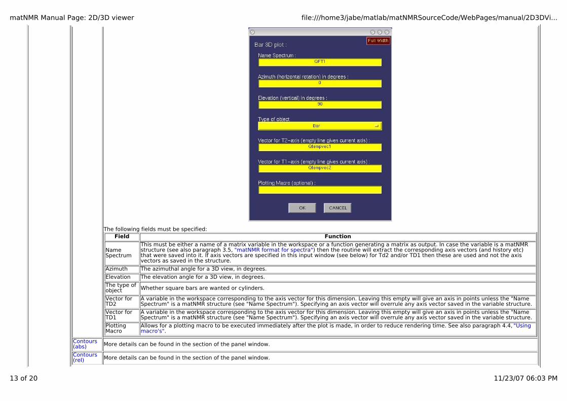
matNMR Manual Page: 2D/3D viewer file:///home3/jabe/matlab/matNMRSourceCode/WebPages/manual/2D3DVi...
13 of 20 11/23/07 06:03 PM
The following fields must be specified:Field Function
Name Spectrum
This must be either a name of a matrix variable in the workspace or a function generating a matrix as output. In case the variable is a matNMRstructure (see also paragraph 3.5, "matNMR format for spectra") then the routine will extract the corresponding axis vectors (and history etc)that were saved into it. If axis vectors are specified in this input window (see below) for Td2 and/or TD1 then these are used and not the axisvectors as saved in the structure.
Azimuth The azimuthal angle for a 3D view, in degrees.
Elevation The elevation angle for a 3D view, in degrees.
The type of object Whether square bars are wanted or cylinders.
Vector for TD2
A variable in the workspace corresponding to the axis vector for this dimension. Leaving this empty will give an axis in points unless the "NameSpectrum" is a matNMR structure (see "Name Spectrum"). Specifying an axis vector will overrule any axis vector saved in the variable structure.
Vector for TD1
A variable in the workspace corresponding to the axis vector for this dimension. Leaving this empty will give an axis in points unless the "NameSpectrum" is a matNMR structure (see "Name Spectrum"). Specifying an axis vector will overrule any axis vector saved in the variable structure.
Plotting Macro
Allows for a plotting macro to be executed immediately after the plot is made, in order to reduce rendering time. See also paragraph 4.4, "Using macro's".
Contours (abs) More details can be found in the section of the panel window.
Contours (rel) More details can be found in the section of the panel window.

matNMR Manual Page: 2D/3D viewer file:///home3/jabe/matlab/matNMRSourceCode/WebPages/manual/2D3DVi...
14 of 20 11/23/07 06:03 PM
Line plot
This function creates a line plot of the 1D spectrum that it requires as input. In case a 2D matrix is given then this results in a series of line plots distributedover the available subplots.The following input window will appear:
The following fields must be specified:Field Function
Name Spectrum
This must be either a name of a matrix variable in the workspace or a function generating a matrix as output. In case the variable is a matNMRstructure (see also paragraph 3.5, "matNMR format for spectra") then the routine will extract the corresponding axis vectors (and history etc) thatwere saved into it. If axis vectors are specified in this input window (see below) for Td2 and/or TD1 then these are used and not the axis vectorsas saved in the structure.
axis Whether or not to print an axis system around the polar plot. Only limited control is available over the axis system currently.
LinespecLeaving this empty will plot the bars as done using the standard line plotting routine in Matlab (for more information on this see the MATLABdocumentation). Specifying the linespec may result in different colours and markers and such. See the MATLAB documentation for moreinformation on linespec properties.
Plotting Macro
Allows for a plotting macro to be executed immediately after the plot is made, in order to reduce rendering time. See also paragraph 4.4, "Using macro's".
Polar plotThis function creates a polar plot using a stereographic projection. A 2D matrix where the dimensions correspond to two polar angles is assumed.The following input window will appear:

matNMR Manual Page: 2D/3D viewer file:///home3/jabe/matlab/matNMRSourceCode/WebPages/manual/2D3DVi...
15 of 20 11/23/07 06:03 PM
The following fields must be specified:Field Function
Name Spectrum
This must be either a name of a matrix variable in the workspace or a function generating a matrix as output. In case the variable is a matNMRstructure (see also paragraph 3.5, "matNMR format for spectra") then the routine will extract the corresponding axis vectors (and history etc) thatwere saved into it. If axis vectors are specified in this input window (see below) for Td2 and/or TD1 then these are used and not the axis vectorsas saved in the structure.
axis Whether or not to print an axis system around the polar plot. Only limited control is available over the axis system currently.
plot typeThis determines whether to print it as a surface (pcolor) or as a contour plot. If the pcolor is chosen then no other options must be given. Ifabsolute contours are asked for then only the vector with contour levels must be given. For relative contours all but the vector of contour levelsmust be given. Please see the corresponding sections for more details on contour plots and surface plots.
Plotting Macro
Allows for a plotting macro to be executed immediately after the plot is made, in order to reduce rendering time. See also paragraph 4.4, "Using macro's".
Raster 2D More details can be found in the section of the panel window.
Surface More details can be found in the section of the panel window.
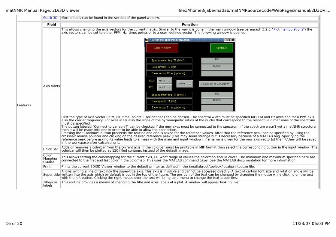
matNMR Manual Page: 2D/3D viewer file:///home3/jabe/matlab/matNMRSourceCode/WebPages/manual/2D3DVi...
16 of 20 11/23/07 06:03 PM
Stack 3D More details can be found in the section of the panel window.
Features
Field Function
Axis rulers
This allows changing the axis vectors for the current matrix. Similar to the way it is done in the main window (see paragraph 5.2.5, "Plot manipulations") the axis vectors can be set to either PPM, Hz, time, points or to a user- defined vector. The following window is opened:
First the type of axis vector (PPM, Hz, time, points, user-defined) can be chosen. The spectral width must be specified for PPM and Hz axes and for a PPM axisalso the carrier frequency. For axes in Hz also the signs of the gyromagnetic ratios of the nuclei that correspond to the respective dimensions of the spectrummust be specified.The button labeled "Connect to variable?" can be checked if the new axes must be connected to the spectrum. If the spectrum wasn't yet a matNMR structurethen it will be made into one in order to be able to allow the connection.Pressing the "Continue" button proceeds the routine and one is asked for the reference values. After that the reference peak can be specified by using thecrosshair mouse pounter and clicking on the desired reference peak (This may seem strange but is necessary because of a MATLAB bug. Specifying thereference peak before asking its value leads to a mess with the main and input window). If a name is given for the new axis vector(s) then it/they will be savedin the workspace after calculating it.
Color Bar Adds or removes a colorbar from the current axis. If the colorbar must be printable in MIF format then select the corresponding button in the input window. Thecolorbar will then be plotted as 150 filled contours instead of the default image.
Color Mapping (caxis)
This allows setting the colormapping for the current axis, i.e. what range of values the colormap should cover. The minimum and maximum specified here areconnected to the first and last color in the colormap. This uses the MATLAB command caxis. See the MATLAB documentation for more information.
Print Prints the current 2D/3D Viewer window to the default printer as defined in the $matlabroot/toolbox/local/printopt.m file.
Super titleAllows writing a line of text into the super-title axis. This axis is invisible and cannot be accessed directly. A text of certain font size and rotation angle will bewritten into the axis which by default is put in the top of the figure. The position of the text can be changed by dragging the mouse while clicking on the textwith the left button. Clicking the right mouse over the text will bring up a menu to change the text properties.
Title/axis labels
This routine provides a means of changing the title and axes labels of a plot. A window will appear looking like:
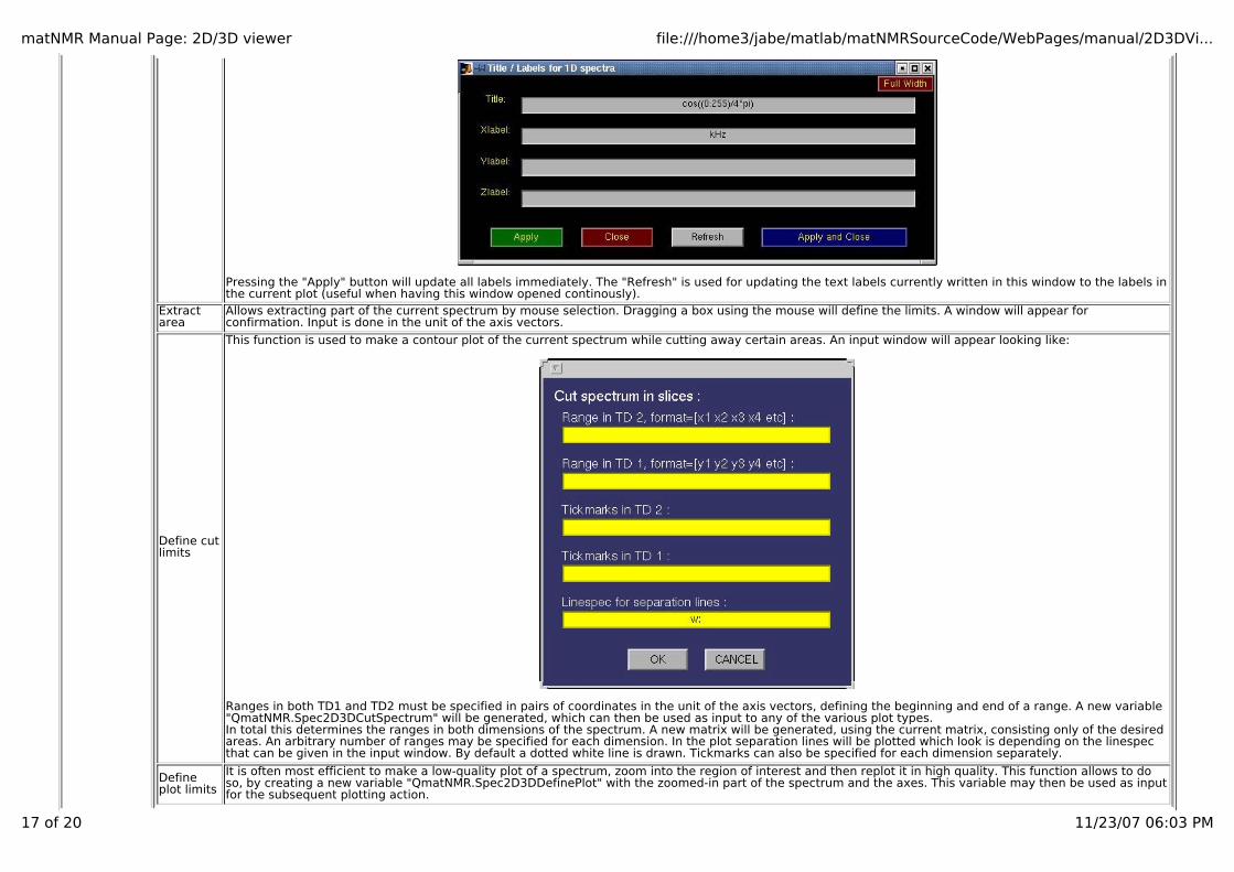
matNMR Manual Page: 2D/3D viewer file:///home3/jabe/matlab/matNMRSourceCode/WebPages/manual/2D3DVi...
17 of 20 11/23/07 06:03 PM
Pressing the "Apply" button will update all labels immediately. The "Refresh" is used for updating the text labels currently written in this window to the labels inthe current plot (useful when having this window opened continously).
Extract area
Allows extracting part of the current spectrum by mouse selection. Dragging a box using the mouse will define the limits. A window will appear forconfirmation. Input is done in the unit of the axis vectors.
Define cut limits
This function is used to make a contour plot of the current spectrum while cutting away certain areas. An input window will appear looking like:
Ranges in both TD1 and TD2 must be specified in pairs of coordinates in the unit of the axis vectors, defining the beginning and end of a range. A new variable"QmatNMR.Spec2D3DCutSpectrum" will be generated, which can then be used as input to any of the various plot types.In total this determines the ranges in both dimensions of the spectrum. A new matrix will be generated, using the current matrix, consisting only of the desiredareas. An arbitrary number of ranges may be specified for each dimension. In the plot separation lines will be plotted which look is depending on the linespecthat can be given in the input window. By default a dotted white line is drawn. Tickmarks can also be specified for each dimension separately.
Define plot limits
It is often most efficient to make a low-quality plot of a spectrum, zoom into the region of interest and then replot it in high quality. This function allows to doso, by creating a new variable "QmatNMR.Spec2D3DDefinePlot" with the zoomed-in part of the spectrum and the axes. This variable may then be used as inputfor the subsequent plotting action.
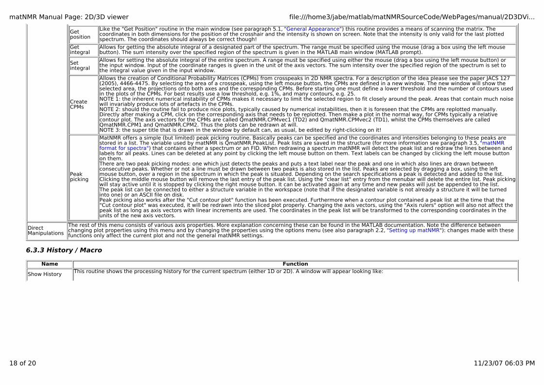
matNMR Manual Page: 2D/3D viewer file:///home3/jabe/matlab/matNMRSourceCode/WebPages/manual/2D3DVi...
18 of 20 11/23/07 06:03 PM
Get position
Like the "Get Position" routine in the main window (see paragraph 5.1, "General Appearance") this routine provides a means of scanning the matrix. Thecoordinates in both dimensions for the position of the crosshair and the intensity is shown on screen. Note that the intensity is only valid for the last plottedspectrum. The coordinates should always be correct though!
Get integral
Allows for getting the absolute integral of a designated part of the spectrum. The range must be specified using the mouse (drag a box using the left mousebutton). The sum intensity over the specified region of the spectrum is given in the MATLAB main window (MATLAB prompt).
Set integral
Allows for setting the absolute integral of the entire spectrum. A range must be specified using either the mouse (drag a box using the left mouse button) orthe input window. Input of the coordinate ranges is given in the unit of the axis vectors. The sum intensity over the specified region of the spectrum is set tothe integral value given in the input window.
Create CPMs
Allows the creation of Conditional Probability Matrices (CPMs) from crosspeaks in 2D NMR spectra. For a description of the idea please see the paper JACS 127(2005), 4466-4475. By selecting the area of a crosspeak, using the left mouse button, the CPMs are defined in a new window. The new window will show theselected area, the projections onto both axes and the corresponding CPMs. Before starting one must define a lower threshold and the number of contours usedin the plots of the CPMs. For best results use a low threshold, e.g. 1%, and many contours, e.g. 25.NOTE 1: the inherent numerical instability of CPMs makes it necessary to limit the selected region to fit closely around the peak. Areas that contain much noisewill invariably produce lots of artefacts in the CPMs. NOTE 2: should the routine fail to produce nice plots, typically caused by numerical instabilities, then it is foreseen that the CPMs are replotted manually.Directly after making a CPM, click on the corresponding axis that needs to be replotted. Then make a plot in the normal way, for CPMs typically a relativecontour plot. The axis vectors for the CPMs are called QmatNMR.CPMvec1 (TD2) and QmatNMR.CPMvec2 (TD1), whilst the CPMs themselves are calledQmatNMR.CPM1 and QmatNMR.CPM2. Thus the plots can be redrawn at will. NOTE 3: the super title that is drawn in the window by default can, as usual, be edited by right-clicking on it!
Peak picking
MatNMR offers a simple (but limited) peak picking routine. Basically peaks can be specified and the coordinates and intensities belonging to these peaks arestored in a list. The variable used by matNMR is QmatNMR.PeakList. Peak lists are saved in the structure (for more information see paragraph 3.5, "matNMR format for spectra") that contains either a spectrum or an FID. When redrawing a spectrum matNMR will detect the peak list and redraw the lines between andlabels for all peaks. Lines can be deleted at any point by clicking the left mouse button on them. Text labels can be changed by clicking the left mouse buttonon them.There are two peak picking modes: one which just detects the peaks and puts a text label near the peak and one in which also lines are drawn betweenconsecutive peaks. Whether or not a line must be drawn between two peaks is also stored in the list. Peaks are selected by dragging a box, using the leftmouse button, over a region in the spectrum in which the peak is situated. Depending on the search specifications a peak is detected and added to the list.Clicking the middle mouse button will remove the last entry of the peak list. Using the "clear list" entry from the menubar will delete the entire list. Peak pickingwill stay active until it is stopped by clicking the right mouse button. It can be activated again at any time and new peaks will just be appended to the list.The peak list can be connected to either a structure variable in the workspace (note that if the designated variable is not already a structure it will be turnedinto one) or an ASCII file on disk.Peak picking also works after the "Cut contour plot" function has been executed. Furthermore when a contour plot contained a peak list at the time that the"Cut contour plot" was executed, it will be redrawn into the sliced plot properly. Changing the axis vectors, using the "Axis rulers" option will also not affect thepeak list as long as axis vectors with linear increments are used. The coordinates in the peak list will be transformed to the corresponding coordinates in theunits of the new axis vectors.
Direct Manipulations
The rest of this menu consists of various axis properties. More explanation concerning these can be found in the MATLAB documentation. Note the difference betweenchanging plot properties using this menu and by changing the properties using the options menu (see also paragraph 2.2, "Setting up matNMR"): changes made with thesefunctions only affect the current plot and not the general matNMR settings.
6.3.3 History / Macro
Name Function
Show History This routine shows the processing history for the current spectrum (either 1D or 2D). A window will appear looking like:

matNMR Manual Page: 2D/3D viewer file:///home3/jabe/matlab/matNMRSourceCode/WebPages/manual/2D3DVi...
19 of 20 11/23/07 06:03 PM
The "Print" button allows to print the history to a printer or to disk. A separate window will be opened in which the history is plotted as graphical text (Unfortunatelt this isnecessary because it is much more difficult to print text in UI-controls than graphical text in MATLAB).
Start recording macro Starts the recording of a new plotting macro (see also paragraph 4.4, "Using macro's").
Stop recording macro
Stop the recording of a macro. An input window will appear to ask for a name of a variable in the workspace to store the new macro in. (see also paragraph 4.4, "Using macro's")
Execute macro This routine executes a macro. (see also paragraph 4.4, "Using macro's")
Execute macro stepwise This routine executes a macro stepwise. The same window as used for "Reprocess from history stepwise" (see above) will appear .
6.3.4 Printing menu
The printing menu is a general feature available from all matNMR windows that is used for printing. Using a separate window the MATLAB print command (see the MATLAB documentationfor more information on print) can be executed. More information on the printing menu is given in paragraph 7.1, "Printing menu".
6.3.5 Copy figure
This function will copy the current view of the main window into a separate window, but without the UI-controls. This will give something like:

matNMR Manual Page: 2D/3D viewer file:///home3/jabe/matlab/matNMRSourceCode/WebPages/manual/2D3DVi...
20 of 20 11/23/07 06:03 PM
The menubar of this new window contains the standard MATLAB menubar which has some useful features for printing and saving the figure. It also offers the possibility to change axisproperties and stuff (More information on this menubar can be found in the MATLAB documentation). Additional features in the menubar are the MATLAB zoom and rotate3D functions, thematNMR "Get Position" (for more information see paragraph 5.1, "General appearance") and the printing menu (for more information see paragraph 7.1, "Printing menu").
6.3.6 Options
This menu contains a subset of matNMR properties that can be changed as for the 2D/3D Viewer not all menus are needed. Please use the menu in the main window for changing all otheroptions. This menu allows changing the default settings of the screen settings and the text properties in matNMR as is described in detail in paragraph 2.2, "Setting up matNMR (options)".
6.3.7 Help
Besides the simple "About matNMR" and "Copyright" notices this contains a direct link to this manual from inside MATLAB. The browser, defined in the $matlabroot/toolbox/local/docopt.mfile, will be opened and the matNMR manual will appear (See the MATLAB documentation for more information on the MATLAB web and docopt commands). As the manual is included in thematNMR distribution reading the manual should be faster than using the matNMR website.
6.3.8 Clear functions
This performs the MATLAB "clear functions" command. All compiled functions are deleted from memory forcing MATLAB to recompile each function again upon running it. This is usefulwhen working with your own m-files (or changing the matNMR code) to force MATLAB to use the altered function (See the MATLAB documentation for more information on the MATLAB clearcommand). Furthermore the mouse pointer is set to an arrow head.
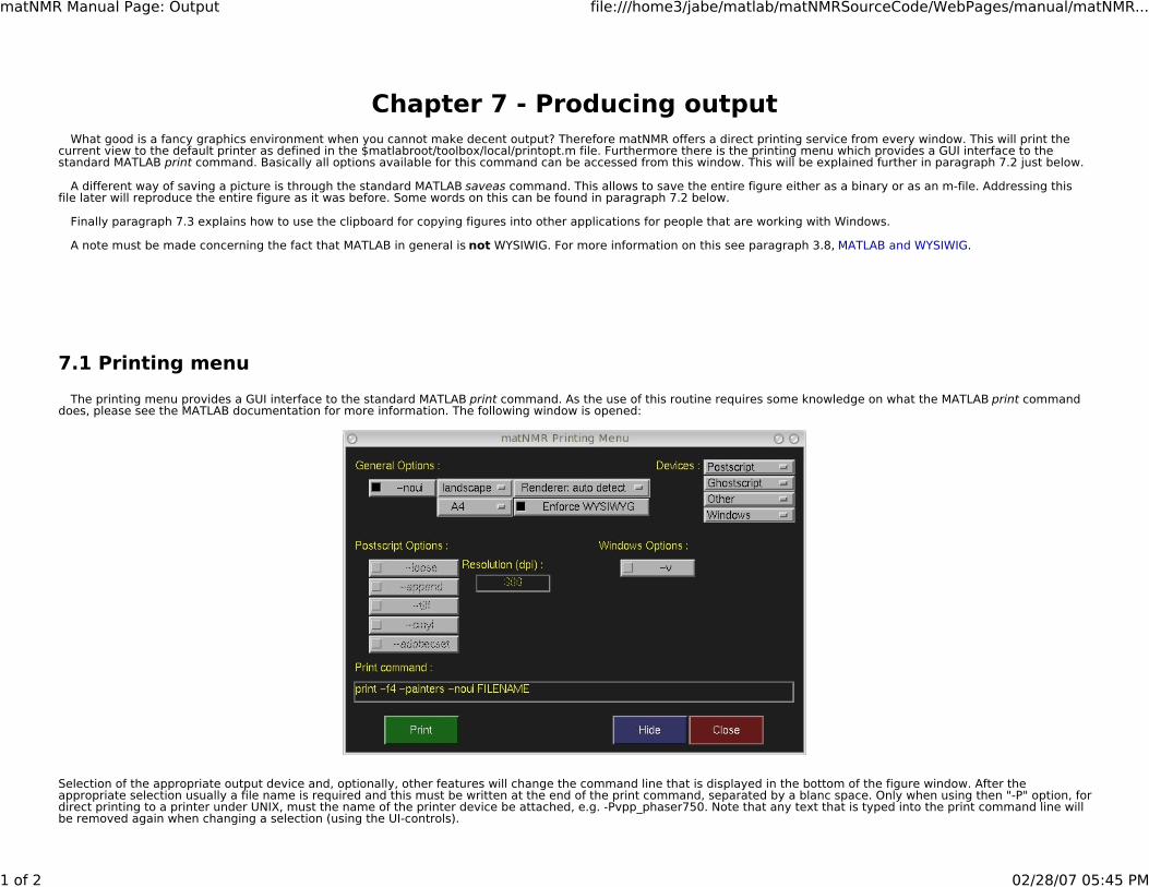
matNMR Manual Page: Output file:///home3/jabe/matlab/matNMRSourceCode/WebPages/manual/matNMR...
1 of 2 02/28/07 05:45 PM
Chapter 7 - Producing outputWhat good is a fancy graphics environment when you cannot make decent output? Therefore matNMR offers a direct printing service from every window. This will print the
current view to the default printer as defined in the $matlabroot/toolbox/local/printopt.m file. Furthermore there is the printing menu which provides a GUI interface to thestandard MATLAB print command. Basically all options available for this command can be accessed from this window. This will be explained further in paragraph 7.2 just below.
A different way of saving a picture is through the standard MATLAB saveas command. This allows to save the entire figure either as a binary or as an m-file. Addressing thisfile later will reproduce the entire figure as it was before. Some words on this can be found in paragraph 7.2 below.
Finally paragraph 7.3 explains how to use the clipboard for copying figures into other applications for people that are working with Windows.
A note must be made concerning the fact that MATLAB in general is not WYSIWIG. For more information on this see paragraph 3.8, MATLAB and WYSIWIG.
7.1 Printing menu
The printing menu provides a GUI interface to the standard MATLAB print command. As the use of this routine requires some knowledge on what the MATLAB print command does, please see the MATLAB documentation for more information. The following window is opened:
Selection of the appropriate output device and, optionally, other features will change the command line that is displayed in the bottom of the figure window. After theappropriate selection usually a file name is required and this must be written at the end of the print command, separated by a blanc space. Only when using then "-P" option, fordirect printing to a printer under UNIX, must the name of the printer device be attached, e.g. -Pvpp_phaser750. Note that any text that is typed into the print command line willbe removed again when changing a selection (using the UI-controls).

matNMR Manual Page: Output file:///home3/jabe/matlab/matNMRSourceCode/WebPages/manual/matNMR...
2 of 2 02/28/07 05:45 PM
The specified paper type and orientation override any current setting for the window that needs to be printed. Plots from default matNMR windows should be centered on theprinted page. The button "enforce WYSIWYG" tries to obtain what-you-see-is-what-you-get behaviour, i.e. make a plot that looks exactly like the window looks on the screen. Incase the absolute size of the window is bigger than the paper size the window will be resized before plotting. As this does not work perfectly in all cases a warning message willbe issued. This states that it is better to resize the window by the given amount yourself. Printing the smaller window should then be really WYSIWYG (at least as far as MATLABallows). For more information see paragraph 3.8, MATLAB and WYSIWIG.
When the print command line is as desired press the "Print" button to execute the command. The figure window is moved into the background and will appear backunchanged when starting the printing menu again.
This menu can also be called from the MATLAB command line by typing "matprint". The routine will assume the current figure as the one to be printed so be sure to make thefigure of interest the current figure (for more information on the MATLAB figure command see the MATLAB documentation).
7.2 Saving figures to disk
The MATLAB command saveas provides a means of saving a figure window to disk in a certain format. As this feature is not specially implemented into matNMR please referto the MATLAB documentation for more information. Note that saving a figure in this way can create very large files!
7.3 Using the clipboard
To copy figures from MATLAB into other applications under Windows requires the standard MATLAB menubar. In general this has been disabled in matNMR because there arequite a few other items that need to be put into the menubars already. Only in the window created after executing the "Copy Figure" command (can be found in the menubar ofall matNMR windows, for a graphical example see paragraph 5.2.8, "Copy Figure") will this MATLAB menubar be present. From there objects can be selected and copied usingthe "Edit" menu.

matNMR Manual Page: Offline Processing file:///home3/jabe/matlab/matNMRSourceCode/WebPages/manual/Offline.h...
1 of 2 11/23/07 06:04 PM
Chapter 8 - Script-based processing with matNMRNOTE: These routines still have not been tested enough yet and can contain minor bugs. Please report any bugs that you find!
It is also possible to use the processing facilities of matNMR in user-defined scripts. A number, but not all, processing actions have been created into separate functions that do not requirethe matNMR GUI to be open. They are, separated by mode:
Mode-independent 1D Processing 2D Processing
matNMRReadBinaryFIDmatNMRReadBrukerSpectramatNMRReadSIMPSONASCIImatNMRTranspose
matNMRApodize1DmatNMRBaselineCorrection1DmatNMRConcatenate1DmatNMRConvertBrukerqseq1DmatNMRDCcorr1DmatNMRExtract1DmatNMRFlip1DmatNMRFT1DmatNMRLeftShift1DmatNMRLP1DmatNMRRegridSpectrum1DmatNMRRemoveBrukerDigitalFilter1DmatNMRSetPhase1DmatNMRSetSize1DmatNMRSolventSuppression1DmatNMRSwapEcho1D
matNMRApodize2DmatNMRConcatenate2DmatNMRConvertBrukerqseq2DmatNMRConvertEAE2DmatNMRConvertStates2DmatNMRDCcorr2DmatNMRExtract2DmatNMRFlip2DmatNMRFT2DmatNMRLeftShift2DmatNMRLP2DmatNMRRegridSpectrum2DmatNMRRemoveBrukerDigitalFilter2DmatNMRSetPhase2DmatNMRSetSize2DmatNMRShearingTransformationFDmatNMRShearingTransformationTDmatNMRSolventSuppression2DmatNMRSymmetrize2DmatNMRSwapEcho2D
The names should be self-explanatory in terms of what the functions do. The syntax for each function can be obtained by typing help "Name Function" in the Matlab command window. This should provide ample information. All the above-mentioned routines operate on matrices only and not on (matNMR) structures! In most cases, processing of hypercomplexmatrices is not supported in the sense that both matrices cannot be entered at the same time, but must be called sequentially from the user-defined script.
It is possible to convert macros to scripts directly from the GUI. This currently only works for 1D actions but this will soon be extended to 2D actions as well.
Note that although most things can be done this way, baseline correction is not (yet) supported as this requires input of peak positions in matNMR. Furthermore, no spectral information ismaintained by these functions.
Finally, an additional way of using matNMR in user-defined scripts is to record processing and/or plotting macro's, which can then be called by the function matNMRRunMacro. Again, thesyntax to this function can be called by typing help matNMRRunMacro in the Matlab command window. This function does require matNMR windows to be open but doesn't rely onuser input whilst processing, i.e. even though changes are made to the matNMR windows they may be hidden from view. This function can be used to either process a spectrum using amacro, OR to execute a plotting macro on the current window.
Here's an example of how one could use matNMRRunMacro in a script:
%%example how to use matNMRRunMacro:%%This file loads all files from the current directory with names Epsilon$#$ where $#$ is a range from 0 to 90.%The FIDs are then processed by macro "m" which was saved in file "Macro.mat". The output variable is called "Spec".%
MacroFile = 'Macro';MacroName = 'm';Range = 0:90;

matNMR Manual Page: Offline Processing file:///home3/jabe/matlab/matNMRSourceCode/WebPages/manual/Offline.h...
2 of 2 11/23/07 06:04 PM
%load file with processing macroeval(['load ' MacroFile]);
%start matNMRnmr
for tel1 = 1:length(Range)%load fileeval(['load Epsilon' num2str(Range(tel1))]);
%process the FIDeval(['MatrixOut = matNMRRunMacro(Epsilon' num2str(Range(tel1)) ', ' MacroName ');']);
%create spectral matrix in first iterationif (tel1 == 1)[x, y] = size(MatrixOut.Spectrum);Spec = zeros(length(Range), x, y);end
%fill in the matrixSpec(tel1, :, :) = MatrixOut.Spectrum;
%clear FID from memoryeval(['clear Epsilon' num2str(Range(tel1))]);end


![Untitled-1 [take-square.com] · Title: Untitled-1 Author: Nikola Created Date: 1/11/2020 6:47:06 PM](https://static.documents.pub/doc/80x56/5f05c7367e708231d414a8d3/untitled-1-take-title-untitled-1-author-nikola-created-date-1112020-64706.jpg)


