1

Online Learning of Rested and Restless BanditsCem Tekin, Mingyan Liu

Department of Electrical Engineering and Computer Science

University of Michigan, Ann Arbor, Michigan, 48109-2122

Email: cmtkn, mingyan@umich.edu

Abstract

In this paper we study the online learning problem involvingrestedandrestlessmultiarmed bandits

with multiple plays. The system consists of a single player/user and a set ofK finite-state discrete-time

Markov chains (arms) with unknown state spaces and statistics. At each time stepthe player can play

M , M ≤ K, arms. The objective of the user is to decide for each step which M of the K arms to

play over a sequence of trials so as to maximize its long term reward. The restless multiarmed bandit is

particularly relevant to the application of opportunisticspectrum access (OSA), where a (secondary) user

has access to a set ofK channels, each of time-varying condition as a result of random fading and/or

certain primary users’ activities.

We first show that a logarithmic regret algorithm exists for therestedmultiarmed bandit problem. We

then construct an algorithm for the restless bandit problemwhich utilizes regenerative cycles of a Markov

chain and computes a sample mean based index policy. We show that under mild conditions on the state

transition probabilities of the Markov chains this algorithm achieves logarithmic regret uniformly over

time, and that this regret bound is also optimal.

I. INTRODUCTION

In this paper we study the online learning problem involvingrestedand restlessmultiarmed bandits

with multiple plays. The system consists of a single player/user and a set ofK finite-state discrete-time

Markov chains (also referred to asarms) with unknown state spaces and statistics. At each time stepthe

player can playM , M ≤ K, arms. Each arm played generates a reward depending on the state the arm

is in when played. The state of an arm is only observed when it is played, and otherwise unknown to

the user. The objective of the user is to decide for each step which M of the K arms to play over a

Preliminary versions of this work appeared in Allerton 2010and Infocom 2011.

2

sequence of trials so as to maximize its long term reward. To do so it must use all its past actions and

observations to essentially learn the quality of each arm (e.g., their expected rewards). We consider two

cases, one withrestedarms where the state of a Markov chain stays frozen unless it’s played, the other

with restlessarms where the state of a Markov chain may continue to evolve (accordingly to a possibly

different law) regardless of the player’s actions.

The above problem is motivated by the following opportunistic spectrum access (OSA) problem. A

(secondary) user has access to a set ofK channels, each of time-varying condition as a result of random

fading and/or certain primary users’ activities. The condition of a channel is assumed to evolve as a

Markov chain. At each time step, the secondary user (simply referred to asthe userfor the rest of the

paper for there is no ambiguity) senses or probesM of the K channels to find out their condition, and

is allowed to use the channels in a way consistent with their conditions. For instance, good channel

conditions result in higher data rates or lower power for theuser and so on. In some cases channel

conditions are simply characterized as being available andunavailable, and the user is allowed to use all

channels sensed to be available. This is modeled as a reward collected by the user, the reward being a

function of the state of the channel or the Markov chain.

The restless bandit model is particularly relevant to this application because the state of each Markov

chain evolves independently of the action of the user. The restless nature of the Markov chains follows

naturally from the fact that channel conditions are governed by external factors like random fading,

shadowing, and primary user activity. In the remainder of this paper a channel will also be referred to

as anarm, the user asplayer, and probing a channel asplaying or selecting an arm.

Within this context, the user’s performance is typically measured by the notion ofregret. It is defined

as the difference between the expected reward that can be gained by an “infeasible” or ideal policy,

i.e., a policy that requires either a priori knowledge of some or all statistics of the arms or hindsight

information, and the expected reward of the user’s policy. The most commonly used infeasible policy

is the best single-actionpolicy, that is optimal among all policies that continue to play the same arm.

An ideal policy could play for instance the arm that has the highest expected reward (which requires

statistical information but not hindsight). This type of regret is sometimes also referred to as theweak

regret, see e.g., work by Auer et al. [1]. In this paper we will only focus on this definition of regret.

Discussion on possibly stronger regret measures is given inSection VI.

This problem is a typical example of the tradeoff betweenexplorationand exploitation. On the one

hand, the player needs to sufficiently explore all arms so as to discover with accuracy the set of best

arms and avoid getting stuck playing an inferior one erroneously believed to be in the set of best arms.

3

On the other hand, the player needs to avoid spending too muchtime sampling the arms and collecting

statistics and not playing the best arms often enough to get ahigh return.

In most prior work on the class of multiarmed bandit problems, originally proposed by Robbins [2], the

rewards are assumed to be independently drawn from a fixed (but unknown) distribution. It’s worth noting

that with this iid assumption on the reward process, whetheran arm is rested or restless is inconsequential

for the following reasons. Since the rewards are independently drawn each time, whether an unselected

arm remains still or continues to change does not affect the reward the arm produces the next time it

is played whenever that may be. This is clearly not the case with Markovian rewards. In the rested

case, since the state is frozen when an arm is not played, the state in which we next observe the arm is

independentof how much time elapses before we play the arm again. In the restless case, the state of

an arm continues to evolve, thus the state in which we next observe it is nowdependenton the amount

of time that elapses between two plays of the same arm. This makes the problem significantly more

difficult.

Below we briefly summarize the most relevant results in the literature. Lai and Robbins in [3] model

rewards as single-parameter univariate densities and givea lower bound on the regret and construct

policies that achieve this lower bound which are calledasymptotically efficientpolicies. This result is

extended by Anantharam et al. in [4] to the case of playing more than one arm at a time. Using a similar

approach Anantharam et al. in [5] develops index policies that are asymptotically efficient for arms with

rewards driven by finite, irreducible, aperiodic and restedMarkov chains with identical state spaces and

single-parameter families of stochastic transition matrices. Agrawal in [6] considers sample mean based

index policies for the iid model that achieveO(log n) regret, wheren is the total number of plays. Auer

et al. in [7] also proposes sample mean based index policies for iid rewards with bounded support; these

are derived from [6], but are simpler than those in [6] and arenot restricted to a specific family of

distributions. These policies achieve logarithmic regretuniformly over time rather than asymptotically in

time, but have bigger constant than that in [3]. In [8] we showed that the index policy in [7] is order

optimal for Markovian rewards drawn from rested arms but notrestricted to single-parameter families,

under some assumptions on the transition probabilities. Parallel to the work presented here, in [9] an

algorithm was constructed that achieves logarithmic regret for the restless bandit problem. The mechanism

behind this algorithm however is quite different from what’s presented here; this difference is discussed

in more detail in Section VI.

Other works such as [10], [11], [12] consider the iid reward case in a decentralized multiplayer setting;

players selecting the same arms experience collision according to a certain collision model. We would

4

like to mention another class of multiarmed bandit problemsin which the statistics of the arms are

known a priori and the state is observed perfectly; these arethus optimization problems rather than

learning problems. The rested case is considered by Gittins[13] and the optimal policy is proved to be

an index policy which at each time plays the arm with highest Gittins’ index. Whittle introduced the

restless version of the bandit problem in [14]. The restlessbandit problem does not have a known general

solution though special cases may be solved. For instance, amyopic policy is shown to be optimal when

channels are identical and bursty in [15] for an OSA problem formulated as a restless bandit problem

with each channel modeled as a two-state Markov chain (the Gilbert-Elliot model).

In this paper we first study the rested bandit problem with Markovian rewards. Specifically, we show

that a straightforward extension of the UCB1 algorithm [7] to the multiple play case (UCB1 was originally

designed for the case of a single play:M = 1) results in logarithmic regret for restless bandits with

Markovian rewards. We then use the key difference between rested and restless bandits to construct a

regenerative cycle algorithm (RCA) that produces logarithmic regret for the restless bandit problem. The

construction of this algorithm allows us to use the proof of the rested problem as a natural stepping

stone, and simplifies the presentation of the main conceptual idea.

The work presented in this paper extends our previous results [8], [16] on single play to multiple

plays (M ≥ 1). Note that this single player model with multiple plays at each time step is conceptually

equivalent to the centralized (coordinated) learning by multiple players, each playing a single arm at

each time step. Indeed our proof takes this latter point of view for ease of exposition, and our results on

logarithmic regret equally applies to both cases.

The remainder of this paper is organized as follows. In Section II we present the problem formulation.

In Section III we analyze a sample mean based algorithm for the rested bandit problem. In Section IV we

propose an algorithm based on regenerative cycles that employs sample mean based indices and analyze

its regret. In Section V we numerically examine the performance of this algorithm in the case of an

OSA problem with Gilbert-Elliot channel model. In Section VI we discuss possible improvements and

compare our algorithm to other algorithms. Section VII concludes the paper.

II. PROBLEM FORMULATION AND PRELIMINARIES

ConsiderK arms (or channels) indexed by the setK = 1, 2, . . . ,K. The ith arm is modeled as a

discrete-time, irreducible and aperiodic Markov chain with finite state spaceSi. There is a stationary and

positive reward associated with each state of each arm. Letrix denote the reward obtained from statex

of arm i, x ∈ Si; this reward is in general different for different states. Let P i =

pixy, x, y ∈ Si

denote

5

the transition probability matrix of thei-th arm, andπi = πix, x ∈ Si the stationary distribution ofP i.

We assume the arms (the Markov chains) are mutually independent. In subsequent sections we will

consider the rested and the restless cases separately. As mentioned in the introduction, the state of a

rested arm changes according toP i only when it is played and remains frozen otherwise. By contrast,

the state of a restless arm changes according toP i regardless of the user’s actions. All the assumptions in

this section applies to both types of arms. We note that the rested model is a special case of the restless

model, but our development under the restless model followsthe rested model1.

Let (P i)′ denote theadjoint of P i on l2(π) where

(pi)′xy = (πiyp

iyx)/πi

x, ∀x, y ∈ Si,

andP i = (P i)′P denotes themultiplicative symmetrizationof P i. We will assume that theP is are such

that P is are irreducible. To give a sense of how weak or strong this assumption is, we first note that

this is a weaker condition than assuming the Markov chains tobe reversible. In addition, we note that

one condition that guarantees theP is are irreducible ispxx > 0,∀x ∈ Si,∀i. This assumption thus holds

naturally for our main motivating application, as it’s possible for channel condition to remain the same

over a single time step (especially if the unit is sufficiently small). It also holds for a very large class

of Markov chains and applications in general. Consider for instance a queueing system scenario where

an arm denotes a server and the Markov chain models its queue length, in which it is possible for the

queue length to remain the same over one time unit.

The mean reward of armi, denoted byµi, is the expected reward of armi under its stationary

distribution:

µi =∑

x∈Si

rixπ

ix . (1)

Consistent with the discrete time Markov chain model, we will assume that the player’s actions occur

in discrete time steps. Time is indexed byt, t = 1, 2, · · · . We will also frequently refer to the time

interval (t− 1, t] as time slott. The player playsM of the K arms at each time step.

Throughout the analysis we will make the additional assumption that the mean reward of armM is

strictly greater than the mean reward of armM + 1, i.e., we haveµ1 ≥ µ2 ≥ · · · ≥ µM > µM+1 ≥

1In general a restless arm may be given by two transition probability matrices, an active one (P i) and a passive one (Qi).The first describes the state evolution when it is played and the second the state evolution when it is not played. When an armmodels channel variation,P i and Qi are in general assumed to be the same as the channel variationis uncontrolled. In thecontext of online learning we shall see that the selection ofQi is irrelevant; indeed the arm does not even have to be Markovianwhen it’s in the passive mode. More is discussed in Section VI.

6

· · · ≥ µK . For rested arms this assumption simplifies the presentation and is not necessary, i.e., results

will hold for µM ≥ µM+1. However, for restless arms the strict inequality betweenµM and µM+1 is

needed because otherwise there can be a large number of arm switchings between theM -th and the

(M + 1)-th arms (possibly more than logarithmic). Strict inequality will prevent this from happening.

We note that this assumption is not in general restrictive; in our motivating application distinct channel

conditions typically means different data rates. Possiblerelaxation of this condition is given in Section

VI.

We will refer to the set of arms1, 2, · · · ,M as theM -best arms and say that each arm in this set is

optimal while referring to the setM + 1,M + 2, · · · ,K as theM -worst arms and say that each arm

in this set issuboptimal.

For a policyα we define its regretRα(n) as the difference between the expected total reward that can

be obtained by only playing theM -best arms and the expected total reward obtained by policyα up to

time n. Let Aα(t) denote the set of arms selected by policyα at t, t = 1, 2, · · · , andxα(t) the state of

arm α(t) ∈ Aα(t) at time t. Then we have

Rα(n) = n

M∑

j=1

µj − Eα

n∑

t=1

∑

α(t)∈Aα(t)

rα(t)xα(t)

. (2)

The objective is to examine how the regretRα(n) behaves as a function ofn for a given policyα and

to construct a policy whose regret is order-optimal, through appropriate bounding. As we will show and

as is commonly done, the key to boundingRα(n) is to bound the expected number of plays of any

suboptimal arm.

Our analysis utilizes the following known results on Markovchains; the proofs are not reproduced

here for brevity. The first result is due to Lezaud [17] that bounds the probability of a large deviation

from the stationary distribution.

Lemma 1: [Theorem 3.3 from [17]] Consider a finite-state, irreducible Markov chainXtt≥1 with

state spaceS, matrix of transition probabilitiesP , an initial distributionq and stationary distributionπ.

Let Nq =∥

∥

∥( qx

πx, x ∈ S)

∥

∥

∥

2. Let P = P ′P be the multiplicative symmetrization ofP whereP ′ is the

adjoint of P on l2(π). Let ǫ = 1− λ2, whereλ2 is the second largest eigenvalue of the matrixP . ǫ will

be referred to as the eigenvalue gap ofP . Let f : S → R be such that∑

y∈S πyf(y) = 0, ‖f‖∞ ≤ 1

and0 < ‖f‖22 ≤ 1. If P is irreducible, then for any positive integern and all0 < γ ≤ 1

P

(∑nt=1 f(Xt)

n≥ γ

)

≤ Nq exp

[

−nγ2ǫ

28

]

.

7

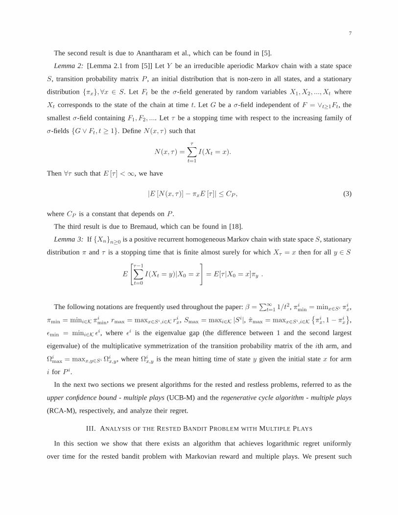
The second result is due to Anantharam et al., which can be found in [5].

Lemma 2: [Lemma 2.1 from [5]] LetY be an irreducible aperiodic Markov chain with a state space

S, transition probability matrixP , an initial distribution that is non-zero in all states, anda stationary

distribution πx,∀x ∈ S. Let Ft be theσ-field generated by random variablesX1,X2, ...,Xt where

Xt corresponds to the state of the chain at timet. Let G be aσ-field independent ofF = ∨t≥1Ft, the

smallestσ-field containingF1, F2, .... Let τ be a stopping time with respect to the increasing family of

σ-fields G ∨ Ft, t ≥ 1. DefineN(x, τ) such that

N(x, τ) =

τ∑

t=1

I(Xt = x).

Then∀τ such thatE [τ ] <∞, we have

|E [N(x, τ)] − πxE [τ ]| ≤ CP , (3)

whereCP is a constant that depends onP .

The third result is due to Bremaud, which can be found in [18].

Lemma 3: If Xnn≥0 is a positive recurrent homogeneous Markov chain with statespaceS, stationary

distributionπ andτ is a stopping time that is finite almost surely for whichXτ = x then for ally ∈ S

E

[

τ−1∑

t=0

I(Xt = y)|X0 = x

]

= E[τ |X0 = x]πy .

The following notations are frequently used throughout thepaper:β =∑∞

t=1 1/t2, πimin = minx∈Si πi

x,

πmin = mini∈K πimin, rmax = maxx∈Si,i∈K ri

x, Smax = maxi∈K |Si|, πmax = maxx∈Si,i∈K

πix, 1 − πi

x

,

ǫmin = mini∈K ǫi, where ǫi is the eigenvalue gap (the difference between 1 and the second largest

eigenvalue) of the multiplicative symmetrization of the transition probability matrix of theith arm, and

Ωimax = maxx,y∈Si Ωi

x,y, whereΩix,y is the mean hitting time of statey given the initial statex for arm

i for P i.

In the next two sections we present algorithms for the restedand restless problems, referred to as the

upper confidence bound - multiple plays(UCB-M) and theregenerative cycle algorithm - multiple plays

(RCA-M), respectively, and analyze their regret.

III. A NALYSIS OF THE RESTED BANDIT PROBLEM WITH MULTIPLE PLAYS

In this section we show that there exists an algorithm that achieves logarithmic regret uniformly

over time for the rested bandit problem with Markovian reward and multiple plays. We present such

8

an algorithm, calledthe upper confidence bound - multiple plays(UCB-M), which is a straightforward

extension of UCB1 from [7]. This algorithm playsM of the K arms with the highest indices with a

modified exploration constantL instead of2 in [7]. Throughout our discussion, we will consider a horizon

of n time slots. For simplicity of presentation we will view a single player playing multiple arms at each

time as multiple coordinated players each playing a single arm at each time. In other words we consider

M players indexed by1, 2, · · · ,M , each playing a single arm at a time. Since in this case information

is centralized, collision is completely avoided among the players, i.e., at each time step an arm will be

played by at most one player.

Below we summarize a list of notations used in this section.

• A(t): the set of arms played at timet (or in slot t).

• T i(t): total number of times (slots) armi is played up to the end of slott.

• T i,j(t): total number of times (slots) playerj played armi up to the end of slott.

• ri(T i(t)): sample mean of the rewards observed from the firstT i(t) plays of armi.

As shown in Figure 1, UCB-M selectsM channels with the highest indices at each time step and

updates the indices according to the rewards observed. The index given on line 4 of Figure 1 depends on

the sample mean reward and an exploration term which reflectsthe relative uncertainty about the sample

mean of an arm. We callL in the exploration termthe exploration constant. The exploration term grows

logarithmically when the arm is not played in order to guarantee that sufficient samples are taken from

each arm to approximate the mean reward.

The Upper Confidence Bound - Multiple Plays (UCB-M):

1: Initialize: Play each armM times in the firstK slots2: while t ≥ K do3: ri(T i(t)) = ri(1)+ri(2)+...+ri(T i(t))

T i(t) , ∀i

4: calculate index:git,T i(t) = ri(T i(t)) +

√

L ln tT i(t) , ∀i

5: t := t + 16: play M arms with the highest indices, updaterj(t) andT j(t).7: end while

Fig. 1. pseudocode for the UCB-M algorithm.

To upper bound the regret of the above algorithm logarithmically, we proceed as follows. We begin

by relating the regret to the expected number of plays of the arms and then show that each suboptimal

arm is played at most logarithmically in expectation. Thesesteps are illustrated in the following lemmas.

Most of these lemmas are established under the following condition on the arms.

9

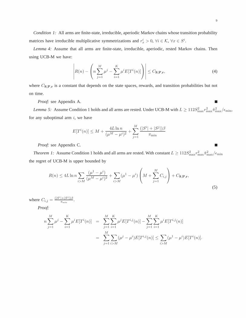
Condition 1: All arms are finite-state, irreducible, aperiodic Markov chains whose transition probability

matrices have irreducible multiplicative symmetrizations andrix > 0, ∀i ∈ K, ∀x ∈ Si.

Lemma 4:Assume that all arms are finite-state, irreducible, aperiodic, rested Markov chains. Then

using UCB-M we have:∣

∣

∣

∣

∣

∣

R(n)−

n

M∑

j=1

µj −K∑

i=1

µiE[T i(n)]

∣

∣

∣

∣

∣

∣

≤ CS,P,r, (4)

whereCS,P,r is a constant that depends on the state spaces, rewards, and transition probabilities but not

on time.

Proof: see Appendix A.

Lemma 5:Assume Condition 1 holds and all arms are rested. Under UCB-Mwith L ≥ 112S2maxr

2maxπ

2max/ǫmin,

for any suboptimal armi, we have

E[T i(n)] ≤M +4L ln n

(µM − µi)2+

M∑

j=1

(|Si|+ |Sj |)β

πmin

Proof: see Appendix C.

Theorem 1:Assume Condition 1 holds and all arms are rested. With constantL ≥ 112S2maxr

2maxπ

2max/ǫmin

the regret of UCB-M is upper bounded by

R(n) ≤ 4L ln n∑

i>M

(µ1 − µi)

(µM − µi)2+∑

i>M

(µ1 − µi)

M +

M∑

j=1

Ci,j

+ CS,P,r,

(5)

whereCi,j = (|Si|+|Sj|)βπmin

.

Proof:

n

M∑

j=1

µj −K∑

i=1

µiE[T i(n)] =

M∑

j=1

K∑

i=1

µjE[T i,j(n)]−M∑

j=1

K∑

i=1

µiE[T i,j(n)]

=M∑

j=1

∑

i>M

(µj − µi)E[T i,j(n)] ≤∑

i>M

(µ1 − µi)E[T i(n)].

10

Thus,

R(n) ≤ n

M∑

j=1

µj −K∑

i=1

µiE[T i(n)] + CS,P,r (6)

≤∑

i>M

(µ1 − µi)E[T i(n)] + CS,P,r

≤∑

i>M

(µ1 − µi)

M +4L ln n

(µM − µi)2+

M∑

j=1

(|Si|+ |Sj |)β

πmin

+ CS,P,r (7)

= 4L ln n∑

i>M

(µ1 − µi)

(µM − µi)2+∑

i>M

(µ1 − µi)

M +

M∑

j=1

Ci,j

+ CS,P,r,

where (6) follows from Lemma 4 and (7) follows from Lemma 5.

The above theorem says that provided thatL satisfies the stated sufficient condition, UCB-M results

in logarithmic regret for the rested problem. This sufficient condition does require certain knowledge on

the underlying Markov chains. This requirement may be removed if the value ofL is adapted over time.

More is discussed in Section VI.

IV. A NALYSIS OF THE RESTLESSBANDIT PROBLEM WITH MULTIPLE PLAYS

In this section we study the restless bandit problem. We construct an algorithm called theregenerative

cycle algorithm - multiple plays(RCA-M), and prove that this algorithm guarantees logarithmic regret

uniformly over time under the same mild assumptions on the state transition probabilities as in the rested

case. RCA-M is a multiple plays extension of RCA first introduced in [16]. Below we first present the key

conceptual idea behind RCA-M, followed by a more detailed pseudocode. We then prove the logarithmic

regret result.

As the name suggests, RCA-M operates in regenerative cycles. In essence RCA-M uses the observations

from sample paths within regenerative cycles to estimate the sample mean of an arm in the form of an

index similar to that used in UCB-M while discarding the restof the observations (only for the computation

of the index, but they are added to the total reward). Note that the rewards from the discarded observations

are collected but are not used to make decisions. The reason behind such a construction has to do with the

restless nature of the arms. Since each arm continues to evolve according to the Markov chain regardless

of the user’s action, the probability distribution of the reward we get by playing an arm is a function

of the amount of time that has elapsed since the last time we played the same arm. Since the arms are

not played continuously, the sequence of observations froman arm which is not played consecutively

does not correspond to a discrete time homogeneous Markov chain. While this certainly does not affect

11

our ability to collect rewards, it becomes hard to analyze the estimated quality (the index) of an arm

calculated based on rewards collected this way.

However, if instead of the actual sample path of observations from an arm, we limit ourselves to a

sample path constructed (or rather stitched together) using only the observations from regenerative cycles,

then this sample path essentially has the same statistics asthe original Markov chain due to the renewal

property and one can now use the sample mean of the rewards from the regenerative sample paths to

approximate the mean reward under stationary distribution.

Under RCA-M each player maintains a block structure; a blockconsists of a certain number of slots.

Recall that as mentioned earlier, even though our basic model is one of single-player multiple-play, our

description is in the equivalent form of multiple coordinated players each with a single play. Within a

block a player plays the same arm continuously till a certainpre-specified state (sayγi) is observed.

Upon this observation the arm enters a regenerative cycle and the player continues to play the same arm

till state γi is observed for the second time, which denotes the end of the block. SinceM arms are

played (byM players) simultaneously in each slot, different blocks overlap in time. Multiple blocks may

or may not start or end at the same time. In our analysis below blocks will be ordered; they are ordered

according to their start time. If multiple blocks start at the same time then the ordering among them is

randomly chosen.

For the purpose of index computation and subsequent analysis, each block is further broken into three

sub-blocks (SBs). SB1 consists of all time slots from the beginning of the block to right before the first

visit to γi; SB2 includes all time slots from the first visit toγi up to but excluding the second visit

to stateγi; SB3 consists of a single time slot with the second visit toγi. Figure 2 shows an example

sample path of the operation of RCA-M. The block structure oftwo players are shown in this example;

the ordering of the blocks is also shown.

The key to the RCA-M algorithm is for each arm to single out only observations within SB2’s in each

block and virtually assemble them. Throughout our discussion, we will consider a horizon ofn time

slots. A list of notations used is summarized as follows:

• A(t): the set of arms played at timet (or in time slott).

• γi: the state that determines the regenerative cycles for armi.

• α(b): the arm played in theb-th block.

• b(n): the total number of completed blocks by all players up to time n.

• T (n): the time at the end of the last completed block across all arms (see Figure 2).

• T i(n): the total number of times (slots) armi is played up to the last completed block of armi up

12

γi γi

γj

γi γi

γj

play arm i play arm i

play arm j

compute index

compute index compute index

compute index

SB1 SB1

SB1

SB2 SB2

SB2

SB3 SB3

SB3

block m block m+1

block m+2

γk γk

play arm k

SB1 SB2 SB3

block m+3

γl γl

play arm l

SB1 SB2 SB3

block m+4(last completed block)

compute index compute index

compute index

time

slot n T(n)

b(n)=m+4

Fig. 2. Example realization of RCA-M withM = 2 for a period ofn slots

to time T (n).

• T i,j(n): the total number of times (slots) armi is played by userj up to the last completed block

of arm i up to timeT (n)

• Bi(b): the total number of blocks within the first completedb blocks in which armi is played.

• Xi1(b): the vector of observed states from SB1 of theb-th block in which armi is played; this vector

is empty if the first observed state isγi.

• Xi2(b): the vector of observed states from SB2 of theb-th block in which armi is played;

• Xi(b): the vector of observed states from theb-th block in which armi is played. Thus we have

Xi(b) = [Xi1(b),X

i2(b), γ

i].

• t(b): time at the end of blockb;

• T i(t(b)): the total number of time slots armi is played up to the last completed block of armi

within time t(b).

• t2(b): the total number of time slots that lie within at least one SB2 in a completed block of any

arm up to and including blockb.

• ri(t): the reward from armi upon itst-th play, counting only those plays during an SB2.

• T i2(t2(b)): the total number of time slots armi is played during SB2’s up to and including blockb.

• O(b): the set of arms that arefree to be selected by some playeri upon its completion of theb-th

13

block; these are arms that are currently not being played by other players (during time slott(b)),

and the arms whose blocks are completed at timet(b).

RCA-M computes and updates the value of anindexgi for each armi in the setO(b) at the end of

block b based on the total reward obtained from armi during all SB2’s as follows:

git2(b),T i

2 (t2(b))= ri(T i

2(t2(b))) +

√

L ln t2(b)

T i2(t2(b))

, (8)

whereL is a constant, and

ri(T i2(t2(b))) =

ri(1) + ri(2) + ... + ri(T i2(t2(b)))

T i2(t2(b))

denotes the sample mean of the reward collected during SB2. Note that this is the same way the index

is computed under UCB-M if we only consider SB2’s. Its also worth noting that under RCA-M rewards

are also collected during SB1’s and SB3’s. However, the computation of the indices only relies on SB2.

The pseudocode of RCA-M is given in Figure 3.

Due to the regenerative nature of the Markov chains, the rewards used in the computation of the index

of an arm can be viewed as rewards from a rested arm with the same transition matrix as the active

transition matrix of the restless arm. However, to prove theexistence of a logarithmic upper bound on

the regret for restless arms remains a non-trivial task since the blocks may be arbitrarily long and the

frequency of arm selection depends on the length of the blocks.

In the analysis that follows, we first show that the expected number of blocks in which a suboptimal

arm is played is at most logarithmic by applying the result inLemma 7 that compares the indices of arms

in slots where an arm is selected. Using this result we then show that the expected number of blocks

in which a suboptimal arm is played is at most logarithmic in time. Using irreducibility of the arms the

expected block length is finite, thus the number of time slotsin which a suboptimal arm is played is

finite. Finally, we show that the regret due to arm switching is at most logarithmic.

We bound the expected number of plays from a suboptimal arm.

Lemma 6:Assume Condition 1 holds and all arms are restless. Under RCA-M with a constantL ≥

112S2maxr

2maxπ

2max/ǫmin, we have

∑

i>M

(µ1 − µi)E[T i(n)] ≤ 4L∑

i>M

(µ1 − µi)Di ln n

(µM − µi)2+∑

i>M

(µ1 − µi)Di

1 + M

M∑

j=1

Ci,j

,

14

The Regenerative Cycle Algorithm - Multiple Plays (RCA-M):

1: Initialize: b = 1, t = 0, t2 = 0, T i2 = 0, ri = 0, Ii

SB2 = 0, IiIN = 1,∀i = 1, · · · ,K, A = ∅

2: //IiIN indicates whether armi has been played at least once

3: //IiSB2 indicates whether armi is in an SB2 sub-block

4: while (1) do5: for i = 1 to K do6: if Ii

IN = 1 and |A| < M then7: A← A∪ i //arms never played is given priority to ensure all arms are sampled initially8: end if9: end for

10: if |A| < M then11: Add to A the set

i : gi is one of theM − |A| largest amonggk, k ∈ 1, · · · ,K −A

12: //for arms that have been played at least once, those with thelargest indices are selected13: end if14: for i ∈ A do15: play armi; denote state observed byxi

16: if IiIN = 1 then

17: γi = xi, T i2 := T i

2 + 1, ri := ri + rixi , Ii

IN = 0, IiSB2 = 1

18: //the first observed state becomes the regenerative state; the arm enters SB219: else if xi 6= γi andIi

SB2 = 1 then20: T i

2 := T i2 + 1, ri := ri + ri

xi

21: else if xi = γi andIiSB2 = 0 then

22: T i2 := T i

2 + 1, ri := ri + rixi , Ii

SB2 = 123: else if xi = γi andIi

SB2 = 1 then24: ri := ri + ri

xi , IiSB2 = 0, A← A− i

25: end if26: end for27: t := t + 1, t2 := t2 + min

1,∑

i∈S IiSB2

//t2 is only accumulated if at least one arm is in SB228: for i = 1 to K do29: gi = ri

T i2

+√

L ln t2T i

2

30: end for31: end while

Fig. 3. Pseudocode of RCA-M

where

Ci,j =(|Si|+ |Sj |)β

πmin, β =

∞∑

t=1

t−2, Di =

(

1

πimin

+ M imax + 1

)

.

Proof: see Appendix E.

We now state the main result of this section.

Theorem 2:Assume Condition 1 holds and all arms are restless. With constantL ≥ 112S2maxr

2maxπ

2max/ǫmin

15

the regret of RCA-M is upper bounded by

R(n) < 4L ln n∑

i>M

1

(µM − µi)2(

(µ1 − µi)Di + Ei

)

+∑

i>M

(

(µ1 − µi)Di + Ei

)

1 + M

M∑

j=1

Ci,j

+ F

where

Ci,j =(|Si|+ |Sj |)β

πmin, β =

∞∑

t=1

t−2

Di =

(

1

πimin

+ M imax + 1

)

,

Ei = µi(1 + M imax) +

M∑

j=1

µjM jmax,

F =

M∑

j=1

µj

(

1

πmin+ max

i∈KM i

max + 1

)

.

Proof: see Appendix F.

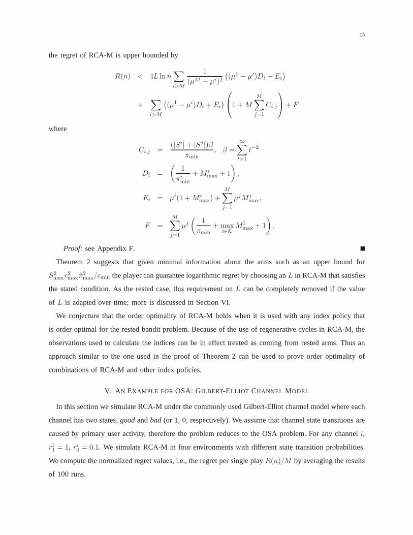
Theorem 2 suggests that given minimal information about thearms such as an upper bound for

S2maxr

2maxπ

2max/ǫmin the player can guarantee logarithmic regret by choosing anL in RCA-M that satisfies

the stated condition. As the rested case, this requirement on L can be completely removed if the value

of L is adapted over time; more is discussed in Section VI.

We conjecture that the order optimality of RCA-M holds when it is used with any index policy that

is order optimal for the rested bandit problem. Because of the use of regenerative cycles in RCA-M, the

observations used to calculate the indices can be in effect treated as coming from rested arms. Thus an

approach similar to the one used in the proof of Theorem 2 can be used to prove order optimality of

combinations of RCA-M and other index policies.

V. A N EXAMPLE FOR OSA: GILBERT-ELLIOT CHANNEL MODEL

In this section we simulate RCA-M under the commonly used Gilbert-Elliot channel model where each

channel has two states,goodandbad (or 1, 0, respectively). We assume that channel state transitions are

caused by primary user activity, therefore the problem reduces to the OSA problem. For any channeli,

ri1 = 1, ri

0 = 0.1. We simulate RCA-M in four environments with different state transition probabilities.

We compute the normalized regret values, i.e., the regret per single playR(n)/M by averaging the results

of 100 runs.

16

The state transition probabilities are given in Table I and the mean rewards of the channels under

these state transition probabilities are given in Table II.The four environment, denoted as S1, S2, S3

and S4, respectively, are summarized as follows. In S1 channels are bursty with mean rewards not close

to each other; in S2 channels are non-bursty with mean rewards not close to each other; in S3 there are

bursty and non-bursty channels with mean rewards not close to each other; and in S4 there are bursty

and non-bursty channels with mean rewards close to each other.

In Figures 4, 6, 8, 10, we observe the normalized regret of RCA-M for the minimum values ofL such

that the logarithmic bound hold. However, comparing with Figures 5, 7, 9, 11 we see that the normalized

regret is smaller forL = 1. Therefore the condition onL we have for the logarithmic bound, while

sufficient, does not appear necessary. We also observe that for the Gilbert-Elliot channel model the regret

can be smaller whenL is set to a value smaller than112S2maxr

2maxπ

2max/ǫmin.

channel 1 2 3 4 5 6 7 8 9 10S1,p01 0.01 0.01 0.02 0.02 0.03 0.03 0.04 0.04 0.05 0.05S1,p10 0.08 0.07 0.08 0.07 0.08 0.07 0.02 0.01 0.02 0.01S2,p01 0.1 0.1 0.2 0.3 0.4 0.5 0.6 0.7 0.8 0.9S2,p10 0.9 0.9 0.8 0.7 0.6 0.5 0.4 0.3 0.2 0.1S3,p01 0.01 0.1 0.02 0.3 0.04 0.5 0.06 0.7 0.08 0.9S3,p10 0.09 0.9 0.08 0.7 0.06 0.5 0.04 0.3 0.02 0.1S4,p01 0.02 0.04 0.04 0.5 0.06 0.05 0.7 0.8 0.9 0.9S4,p10 0.03 0.03 0.04 0.4 0.05 0.06 0.6 0.7 0.8 0.9

TABLE ITRANSITION PROBABILITIES

channel 1 2 3 4 5 6 7 8 9 10S1 0.20 0.21 0.28 0.30 0.35 0.37 0.70 0.82 0.74 0.85S2 0.19 0.19 0.28 0.37 0.46 0.55 0.64 0.73 0.82 0.91S3 0.19 0.19 0.28 0.37 0.46 0.55 0.64 0.73 0.82 0.91S4 0.460 0.614 0.550 0.600 0.591 0.509 0.585 0.580 0.577 0.550

TABLE IIMEAN REWARDS

17

0 1 2 3 4 5 6 7 8 9 10

x 104

0

500

1000

1500

2000

2500

3000

n

R(n

)/(M

ln(n

))

M=1M=2M=3M=4M=5

Fig. 4. Normalized regret under S1,L = 7200

0 1 2 3 4 5 6 7 8 9 10

x 104

−20

0

20

40

60

80

100

120

140

160

180

n

R(n

)/(M

ln(n

))

M=1M=2M=3M=4M=5

Fig. 5. Normalized regret under S1,L = 1

0 1 2 3 4 5 6 7 8 9 10

x 104

0

500

1000

1500

2000

2500

n

R(n

)/(M

ln(n

))

M=1M=2M=3M=4M=5

Fig. 6. Normalized regret under S2,L = 360

0 1 2 3 4 5 6 7 8 9 10

x 104

0

10

20

30

40

50

60

n

R(n

)/(M

ln(n

))

M=1M=2M=3M=4M=5

Fig. 7. Normalized regret under S2,L = 1

VI. D ISCUSSION

In this section we discuss how the performance of RCA-M may beimproved (in terms of the constants

and not in order), and possible relaxation and extensions.

A. Applicability, Performance Improvement, and Relaxation

We note that the same logarithmic bound derived in this paperholds for the general restless bandit

where the state evolution is given by two matrices: the active and passive transition probability matrices

(P i andQi respectively for armi), which are potentially different. The addition of a different Qi does

not affect the analysis because the reward to the player froman arm is determined only by the active

18

transition probability matrix and the first state after a discontinuity in playing the arm. Since the number

of plays from any suboptimal arm is logarithmic and the expected hitting time of any state is finite the

regret due toQi is at most logarithmic. We further note that for the same reason the arm may not even

follow a Markovian rule in the passive state, and the same logarithmic bound will continue to hold.

The regenerative state for an arm under RCA-M is chosen basedon the random initial observation.

This means that RCA-M may happen upon a state with long recurrence time which will result in long

SB1 and SB2 sub-blocks. We propose the following modification: RCA-M records all observations from

all arms. Letki(s, t) be the total number of observations from armi up to timet that areexcludedfrom

the computation of the index of armi when the regenerative state iss. Recall that the index of an arm is

computed based on observations from regenerative cycles; this implies thatki(s, t) is the total number of

slots in SB1’s when the regenerative state iss. Let tn be the time at the end of then-th block. If the arm

to be played in then-th block is i then the regenerative state is set toγi(n) = arg mins∈Si ki(s, tn−1).

The idea behind this modification is to estimate the state with the smallest recurrence time and choose

the regenerative cycles according to this state. With this modification the number of observations that

does not contribute to the index computation and the probability of choosing a suboptimal arm can be

minimized over time.

It’s also worth noting that the selection of the regenerative stateγi in each block in general can be

arbitrary: within the same SB2, we can start and end in different states. As long as we guarantee that

two successive SB2’s end and start with the same state, we will have a continuous sample path for which

our analysis in Section IV holds.

0 1 2 3 4 5 6 7 8 9 10

x 104

0

500

1000

1500

2000

2500

3000

3500

n

R(n

)/(M

ln(n

))

M=1M=2M=3M=4M=5

Fig. 8. Normalized regret under S3,L = 3600

0 1 2 3 4 5 6 7 8 9 10

x 104

0

10

20

30

40

50

60

70

80

n

R(n

)/(M

ln(n

))

M=1M=2M=3M=4M=5

Fig. 9. Normalized regret under S3,L = 1

19

0 1 2 3 4 5 6 7 8 9 10

x 104

0

50

100

150

200

250

300

350

400

450

500

n

R(n

)/ln

(n)

M=1M=2M=3M=4M=5

Fig. 10. Normalized regret under S4,L = 7200

0 1 2 3 4 5 6 7 8 9 10

x 104

−10

0

10

20

30

40

50

60

70

n

R(n

)/ln

(n)

M=1M=2M=3M=4M=5

Fig. 11. Normalized regret under S4,L = 1

B. Relaxation of Certain Conditions

We have noted in Section V that the condition onL while sufficient does not appear necessary for

the logarithmic regret bound to hold. Indeed our examples show that smaller regret can be achieved by

settingL = 1. Note that this condition onL originates from the large deviation bound by Lezaud given

in Lemma 1. This condition can be relaxed if we use a tighter large deviation bound.

We further note that even if no information is available on the underlying Markov chains to derive

this sufficient condition onL, ano(log(n)f(n)) regret is achievable by lettingL grow slowly with time

wheref(n) is any increasing sequence. Such approach has been used in other settings and algorithms,

see e.g., [11], [9].

We have noted earlier that the strict inequalityµM > µM+1 is required for the restless multiarmed

bandit problem because in order to have logarithmic regret,we can have no more than a logarithmic

number of discontinuities from the optimal arms. WhenµM = µM+1 the rankings of the indices of arms

M andM + 1 can oscillate indefinitely resulting in a large number of discontinuities. Below we briefly

discuss how to resolve this issue if indeedµM = µM+1. Consider adding a thresholdǫ to the algorithm

such that a new arm will be selected instead of an arm currently being played only if the index of that

arm is at leastǫ larger than the index of the currently played arm which has the smallest index among

all currently played arms. Then given thatǫ is sufficiently small (with respect to the differences of mean

rewards) indefinite switching between theM -th and theM +1-th arms can be avoided. However, further

analysis is needed to verify that this approach will result in logarithmic regret.

20

C. Definition of Regret

We have used the weak regret measure throughout this paper, which compares the learning strategy

with the best single-action strategy. When the statistics are known a priori, it is clear that in general the

best one can do is not a single-action policy (in principle one can drive such a policy using dynamic

programming). Ideally one could try to adopt a regret measure with respect to this optimal policy.

However, such an optimal policy in the restless case is not known in general [14], [19], which makes

the comparison intractable, except for some very limited cases when such a policy happens to be known

[15], [20].

D. Extensions to A Decentralized Multiplayer Setting and Comparison with Similar Work

As mentioned in the introduction, there has been a number of recent studies extending single player

algorithms to multi-player settings where collisions are possible [21], [11]. Within this context we note

that RCA-M in its currently form does not extend in a straightforward way to a decentralized multi-

player setting. It remains an interesting subject of futurestudy. A recent work [9] considers the same

restless multiarmed bandit problem studied in the present paper. They achieve logarithmic regret by using

exploration and exploitation blocks that grow geometrically with time. The construction in [9] is very

different from ours, but is amenable to multi-player extension [21] due to the constant, though growing,

nature of the block length which can be synchronized among players.

It is interesting to note that the essence behind our approach RCA-M is to reduce a restless bandit

problem to a rested bandit problem; this done by sampling in away to construct a continuous sample

path, which then allows us to use the same set of large deviation bounds over this reconstructed, entire

sample path. By contrast, the method introduced in [9] applies large deviation bounds to individual

segments (blocks) of the observed sample path (which is not acontinuous sample path representative of

the underlying Markov chain because the chain is restless);this necessitates the need to precisely control

the length and the number of these blocks, i.e., they must grow in length over time. Another difference

is that under our scheme, the exploration and exploitation are done simultaneously and implicitly through

the use of the index, whereas under the scheme in [9], the two are done separately and explicitly through

two different types of blocks.

VII. C ONCLUSION

In this paper we considered the rested and restless multiarmed bandit problem with Markovian rewards

and multiple plays. We showed that a simple extension to UCB1produces logarithmic regret uniformly

21

over time. We then constructed an algorithm RCA-M that utilizes regenerative cycles of a Markov chain

to compute a sample mean based index policy. The sampling approach reduces a restless bandit problem

to the rested version, and we showed that under mild conditions on the state transition probabilities of

the Markov chains this algorithm achieves logarithmic regret uniformly over time for the restless bandit

problem, and that this regret bound is also optimal. We numerically examine the performance of this

algorithm in the case of an OSA problem with the Gilbert-Elliot channel model.

REFERENCES

[1] P. Auer, N. Cesa-Bianchi, Y. Freund, and R. Schapire, “The nonstochastic multiarmed bandit problem,”SIAM Journal on

Computing, vol. 32, pp. 48–77, 2002.

[2] H. Robbins, “Some aspects of the sequential design of experiments,”Bull. Amer. Math. Soc., vol. 55, pp. 527–535, 1952.

[3] T. Lai and H. Robbins, “Asymptotically efficient adaptive allocation rules,”Advances in Applied Mathematics, vol. 6, pp.

4–22, 1985.

[4] V. Anantharam, P. Varaiya, and J. . Walrand, “Asymptotically efficient allocation rules for the multiarmed bandit problem

with multiple plays-Part I: IID rewards,”IEEE Trans. Automat. Contr., pp. 968–975, November 1987.

[5] ——, “Asymptotically efficient allocation rules for the multiarmed bandit problem with multiple plays-Part II: Markovian

rewards,”IEEE Trans. Automat. Contr., pp. 977–982, November 1987.

[6] R. Agrawal, “Sample mean based index policies with o(logn) regret for the multi-armed bandit problem,”Advances in

Applied Probability, vol. 27, no. 4, pp. 1054–1078, December 1995.

[7] P. Auer, N. Cesa-Bianchi, and P. Fischer, “Finite-time analysis of the multiarmed bandit problem,”Machine Learning,

vol. 47, p. 235256, 2002.

[8] C. Tekin and M. Liu, “Online algortihms for the multi-armed bandit problem with markovian rewards,” inAllerton

Conference, 2010.

[9] H. Liu, K. Liu, and Q. Zhao, “Learning in a changing world:Non-bayesian restless multi-armed bandit,”Techinal Report,

UC Davis, October 2010.

[10] K. Liu and Q. Zhao, “Distributed learning in multi-armed bandit with multiple players,” vol. 58, no. 11, pp. 5667–5681,

November 2010.

[11] A. Anandkumar, N. Michael, A. Tang, and A. Swami, “Distributed algorithms for learning and cognitive medium access

with logarithmic regret,” 2010.

[12] Y. Gai, B. Krishnamachari, and R. Jain, “Learning multiuser channel allocations in cognitive radio networks: a combinatorial

multi-armed bandit formulation,” inIEEE Symp. on Dynamic Spectrum Access Networks (DySPAN), April 2010.

[13] J. Gittins, “Bandit processes and dynamic allocation indices,”Journal of the Royal Statistical Society, vol. 41, no. 2, pp.

148–177, 1979.

[14] P. Whittle, “Restless bandits: : Activity allocation in a changing world,”A Celebration of Applied Probability, ed. J. Gani,

Journal of applied probability, vol. 25A, pp. 287–298, 1988.

[15] S. H. A. Ahmad, M. Liu, T. Javidi, Q. Zhao, and B. Krishnamachari, “Optimality of myopic sensing in multi-channel

opportunistic access,”IEEE Transactions on Information Theory, vol. 55, no. 9, pp. 4040–4050, September 2009.

[16] C. Tekin and M. Liu, “Online learning in opportunistic spectrum access: A restless bandit approach,”IEEE INFOCOM,

April 2011.

22

[17] P. Lezaud, “Chernoff-type bound for finite markov chains,” Ann. Appl. Prob., vol. 8, pp. 849–867, 1998.

[18] P. Bremaud,Markov Chains, Gibbs Fields, Monte Carlo Simulation and Queues. Springer, 1998.

[19] J. T. C. Papadimitriou, “The complexity of optimal queuing network control,”Mathematics of Operations Research, vol. 24,

no. 2, pp. 293–305, May 1999.

[20] W. Dai, Y. Gai, B. Krishnamachari, and Q. Zhao, “The non-bayesian restless multi-armed bandit: A case of near-logarithmic

regret,” Proc. of Internanional Conference on Acoustics, Speech andSignal Processing (ICASSP), May 2011.

[21] H. Liu, K. Liu, and Q. Zhao, “Learning and sharing in a changing world: Non-bayesian restless bandit with multiple

players,”Proc. of Information Theory and Applications Workshop (ITA), January 2011.

APPENDIX A

PROOF OFLEMMA 4

Let Xi,j(t) be the state observed from thetth play of armi by player j and T i,j(n) be the total

number of times playerj played armi up to and including timen. Then we have,

∣

∣

∣

∣

∣

∣

R(n)−

n

M∑

j=1

µj −K∑

i=1

µiE[T i(n)]

∣

∣

∣

∣

∣

∣

=

∣

∣

∣

∣

∣

∣

E

M∑

j=1

K∑

i=1

∑

x∈Si

rix

T i,j(n)∑

t=1

I(Xi,j(t) = x)

−M∑

j=1

K∑

i=1

∑

x∈Si

rixπi

xE[T i,j(n)]

∣

∣

∣

∣

∣

∣

=

∣

∣

∣

∣

∣

∣

M∑

j=1

K∑

i=1

∑

x∈Si

rix(E[N j(x, T i,j(n))]− πi

xE[T i,j(n)])

∣

∣

∣

∣

∣

∣

≤M∑

j=1

K∑

i=1

∑

x∈Si

rixCP i = CS,P,r (9)

where

N j(x, T i,j(n)) =

T i,j(n)∑

t=1

I(Xi,j(t) = x),

and (9) follows from Lemma 2 using the fact thatT i,j(n) is a stopping time with respect to theσ-field

generated by the arms played up to timen.

APPENDIX B

Lemma 7:Assume Condition 1 holds and all arms are rested. Letgit,s = ri(s)+ct,s, ct,s =

√

L ln t/s.

Under UCB-M with constantL ≥ 112S2maxr

2maxπ

2max/ǫmin, for any suboptimal armi and optimal armj

23

we have

E

n∑

t=1

t−1∑

w=1

t−1∑

wi=l

I(gjt,w ≤ gi

t,wi)

≤|Si|+ |Sj |

πminβ, (10)

wherel =⌈

4L lnn(µM−µi)2

⌉

andβ =∑∞

t=1 t−2.

Proof: First, we show that for any suboptimal armi and optimal armj, we have thatgjt,w ≤ gi

t,wi

implies at least one of the following holds:

rj(w) ≤ µj − ct,w (11)

ri(wi) ≥ µi + ct,wi(12)

µj < µi + 2ct,wi. (13)

This is because if none of the above holds, then we must have

gjt,w = rj(w) + ct,w > µj ≥ µi + 2ct,wi

> ri(wi) + ct,wi= gi

t,wi,

which contradictsgjt,w ≤ gi

t,wi.

If we choosewi ≥ 4L ln n/(µM − µi)2, then

2ct,wi= 2

√

L ln t

wi≤ 2

√

L ln t(µM − µi)2

4L ln n≤ µj − µi for t ≤ n,

which means (13) is false, and therefore at least one of (11) and (12) is true with this choice ofwi. Let

l =⌈

4L lnn(µM−µi)2

⌉

. Then we have,

E

n∑

t=1

t−1∑

w=1

t−1∑

wi=l

I(gjt,w ≤ gi

t,wi)

≤n∑

t=1

t−1∑

w=1

t−1∑

wi=l

4L ln n

(µM −µi)2

m

(

P (rj(w) ≤ µj − ct,w) + P (ri(wi) ≥ µi + ct,wi))

≤∞∑

t=1

t−1∑

w=1

t−1∑

wi=l

4L ln n

(µM −µi)2

m

(

P (rj(w) ≤ µj − ct,w) + P (ri(wi) ≥ µi + ct,wi))

.

Consider an initial distributionqi for the ith arm. We have:

Nqi =

∥

∥

∥

∥

∥

(

qiy

πiy

, y ∈ Si

)∥

∥

∥

∥

∥

2

≤∑

y∈Si

∥

∥

∥

∥

∥

qiy

πiy

∥

∥

∥

∥

∥

2

≤1

πmin,

24

where the first inequality follows from the Minkowski inequality. Let niy(t) denote the number of times

statey of arm i is observed up to and including thet-th play of armi.

P (ri(wi) ≥ µi + ct,wi)

= P

∑

y∈Si

riyn

iy(wi) ≥ wi

∑

y∈Si

riyπ

iy + wict,wi

= P

∑

y∈Si

(riyn

iy(wi)− wir

iyπ

iy) ≥ wict,wi

= P

∑

y∈Si

(−riyn

iy(wi) + wir

iyπ

iy) ≤ −wict,wi

. (14)

Consider a sample pathω and the events

A =

ω :∑

y∈Si

(−riyn

iy(wi)(ω) + wir

iyπ

iy) ≤ −wict,wi

,

B =⋃

y∈Si

ω : −riyn

iy(wi)(ω) + wir

iyπ

iy ≤ −

wict,wi

|Si|

.

If ω /∈ B, then

−riyn

iy(wi)(ω) + wir

iyπ

iy > −

wict,wi

|Si|, ∀y ∈ Si

⇒∑

y∈Si

(−riyn

iy(wi)(ω) + wir

iyπ

iy) > −wict,wi

.

Thusω /∈ A, thereforeP (A) ≤ P (B). Then continuing from (14):

P (ri(wi) ≥ µi + ct,wi)

≤∑

y∈Si

P

(

−riyn

iy(wi) + wir

iyπ

iy ≤ −

wict,wi

|Si|

)

=∑

y∈Si

P

(

riyn

iy(wi)− wir

iyπ

iy ≥

wict,wi

|Si|

)

= P

(

niy(wi)− wiπ

iy ≥

wict,wi

|Si|riy

)

25

= P

(

∑wi

t=1 I(Xit = y)− wiπ

iy

πiywi

≥ct,wi

|Si|riyπ

iy

)

≤∑

y∈Si

Nqit− Lǫi

28(|Si|riyπi

y)2 (15)

≤|Si|

πmint−

Lǫmin28S2

maxr2maxπ2

max , (16)

where (15) follows from Lemma 1 by letting

γ =ct,wi

|Si|riyπ

iy

, f(Xit) =

I(Xit = y)− πi

y

πiy

,

and recallingπiy = maxπi

y, 1− πiy (note P i is irreducible).

Similarly, we have

P(

rj(w) ≤ µj − ct,w

)

= P

∑

y∈Sj

rjy(n

jy(w)− wπj

y) ≤ −wct,w

≤∑

y∈Sj

P

(

rjyn

jy(w)− wrj

yπjy ≤ −

wct,w

|Sj|

)

=∑

y∈Sj

P

rjy(w −

∑

x 6=y

njx(w))− wrj

y(1−∑

x 6=y

πjx) ≤ −

wct,w

|Sj |

=∑

y∈Sj

P

rjy

∑

x 6=y

njx(w) − wrj

y

∑

x 6=y

πjx ≥

wct,w

|Sj |

≤∑

y∈Sj

Nqj t− Lǫj

28(|Sj |rjyπ

jy)2 (17)

≤|Sj |

πmint−

Lǫmin28S2

maxr2maxπ2

max (18)

where (17) again follows from Lemma 1. The result then follows from combining (16) and (18):

E

n∑

t=1

t−1∑

w=1

t−1∑

wi=l

I(gjt,w ≤ gi

t,wi)

≤|Si|+ |Sj |

πmin

∞∑

t=1

t−1∑

w=1

t−1∑

wi=1

t−

Lǫmin28S2

maxr2maxπ2

max

=|Si|+ |Sj |

πmin

∞∑

t=1

t−

Lǫmin−56S2maxr2

maxπ2max

28S2maxr2

maxπ2max

≤|Si|+ |Sj |

πmin

∞∑

t=1

t−2. (19)

26

APPENDIX C

PROOF OFLEMMA 5

Let l be any positive integer and consider a suboptimal armi. Then,

T i(n) = M +

n∑

t=K+1

I(i ∈ A(t)) ≤M − 1 + l +

n∑

t=K+1

I(i ∈ A(t), T i(t− 1) ≥ l) . (20)

Consider

E =

M⋃

j=1

gjt,T j(t) ≤ gi

t,T i(t)

,

and

EC =M⋂

j=1

gjt,T j(t) > gi

t,T i(t)

.

If w ∈ EC then i /∈ A(t). Thereforei ∈ A(t) ⊂ E and

I(i ∈ A(t), T i(t− 1) ≥ l) ≤ I(ω ∈ E, T i(t− 1) ≥ l)

≤M∑

j=1

I(gjt,T j(t) ≤ gi

t,T i(t), T i(t− 1) ≥ l).

Therefore continuing from (20),

T i(n) ≤ M − 1 + l +

M∑

j=1

n∑

t=K+1

I(gjt,T j(t) ≤ gi

t,T i(t), Ti(t− 1) ≥ l)

≤ M − 1 + l +

M∑

j=1

n∑

t=K+1

I

(

min1≤w≤t

gjt,w ≤ max

l≤wi≤tgit,wi

)

≤ M − 1 + l +

M∑

j=1

n∑

t=K+1

t−1∑

w=1

t−1∑

wi=l

I(gjt,w ≤ gi

t,wi)

≤ M − 1 + l +

M∑

j=1

n∑

t=1

t−1∑

w=1

t−1∑

wi=l

I(gjt,w ≤ gi

t,wi).

(21)

27

Using Lemma 7 withl =⌈

4L lnn(µM−µi)2

⌉

, we have for any suboptimal arm

E[T i(n)] ≤M +4L ln n

(µM − µi)2+

M∑

j=1

(|Si|+ |Sj|)β

πmin. (22)

APPENDIX D

Lemma 8:Assume Condition 1 holds and all arms are restless. Letgit,w = ri(w) + ct,w, ct,w =

√

L ln t/w. Under RCA-M with constantL ≥ 112S2maxr

2maxπ

2max/ǫmin, for any suboptimal armi and

optimal armj we have

E

t2(b)∑

t=1

t−1∑

w=1

t−1∑

wi=l

I(gjt,w ≤ gi

t,wi)

≤|Si|+ |Sj|

πminβ, (23)

wherel =⌈

4L lnn(µM−µi)2

⌉

and,β =∑∞

t=1 t−2.

Proof: Note that all the quantities in computing the indices in (23)comes from the intervals

Xi2(1),X

i2(2), · · · ∀i ∈ 1, · · · ,K. Since these intervals begin with stateγi and end with a return

to γi (but excluding the return visit toγi), by the strong Markov property the process at these stopping

times have the same distribution as the original process. Moreover by connecting these intervals together

we form a continuous sample path which can be viewed as a sample path generated by a Markov chain

with an transition matrix identical to the original arm. Therefore we can proceed in exactly the same

way as the proof of Lemma 7. If we choosesi ≥ 4L ln(n)/(µM − µi)2, then for t ≤ t2(b) = n′ ≤ n,

and for any suboptimal armi and optimal armj,

2ct,si= 2

√

L ln(t)

si≤ 2

√

L ln(t)(µM − µi)2

4L ln(n)≤ µj − µi.

The result follows from lettingl =⌈

4L ln n(µM−µi)2

⌉

and using Lemma 7.

APPENDIX E

PROOF OFLEMMA 6

Let ct,w =√

L ln t/w, and letl be any positive integer. Then,

Bi(b) = 1 +

b∑

m=K+1

I(α(m) = i) ≤ l +

b∑

m=K+1

I(α(m) = i, Bi(m− 1) ≥ l) (24)

28

Consider any sample pathω and the following sets

E =M⋃

j=1

ω : gj

t2(m−1),T j

2 (t2(m−1))(ω) ≤ gi

t2(m−1),T i2 (t2(m−1))(ω)

,

and

EC =

M⋂

j=1

ω : gj

t2(m−1),T j2 (t2(m−1))

(ω) > git2(m−1),T i

2 (t2(m−1))(ω)

.

If ω ∈ EC thenα(m) 6= i. Thereforeω : α(m)(ω) = i ⊂ E and

I(α(m) = i, Bi(m− 1) ≥ l) ≤ I(ω ∈ E,Bi(m− 1) ≥ l)

≤M∑

j=1

I(gj

t2(m−1),T j

2 (t2(m−1))≤ gi

t2(m−1),T i2 (t2(m−1)), B

i(m− 1) ≥ l) .

Therefore continuing from (24),

Bi(b) ≤ l +M∑

j=1

b∑

m=K+1

I(gj

t2(m−1),T j

2 (t2(m−1))≤ gi

t2(m−1),T i2 (t2(m−1)), B

i(m− 1) ≥ l)

≤ l +

M∑

j=1

b∑

m=K+1

I

(

min1≤w≤t2(m−1)

gjt2(m−1),w ≤ max

t2(l)≤wi≤t2(m−1)git2(m−1),wi

)

≤ l +

M∑

j=1

b∑

m=K+1

t2(m−1)∑

w=1

t2(m−1)∑

wi=t2(l)

I(gjt2(m),w ≤ gi

t2(m),wi) (25)

≤ l + MM∑

j=1

t2(b)∑

t=1

t−1∑

w=1

t−1∑

wi=l

I(gjt,w ≤ gi

t,wi) , (26)

where as given in (8),git,w = ri(w) + ct,w, and we have assumed that the index value of an arm remains

the same between two updates. The inequality in (26) followsfrom the facts that the second outer sum

in (26) is over time while the second outer sum in (25) is over blocks, each block lasts at least two time

slots and at mostM blocks can be completed in each time step. From this point on we use Lemma 8 to

get

E[Bi(b(n))|b(n) = b] ≤

⌈

4L ln t2(b)

(µM − µi)2

⌉

+ M

M∑

j=1

(|Si|+ |Sj |)β

πmin,

for all suboptimal arms. Therefore,

E[Bi(b(n))] ≤4L ln n

(µM − µi)2+ 1 + M

M∑

j=1

Ci,jβ, (27)

29

sincen ≥ t2(b(n)) almost surely.

The total number of plays of armi at the end of blockb(n) is equal to the total number of plays of

arm i during the regenerative cycles of visiting stateγi plus the total number of plays before entering

the regenerative cycles plus one more play resulting from the last play of the block which is stateγi.

This gives:

E[T i(n)] ≤

(

1

πimin

+ Ωimax + 1

)

E[Bi(b(n))] .

Thus,

∑

i>M

(µ1 − µi)E[T i(n)] (28)

≤ 4L∑

i>M

(µ1 − µi)Di ln n

(µM − µi)2+∑

i>M

(µ1 − µi)Di

1 + MM∑

j=1

Ci,j

. (29)

APPENDIX F

PROOF OFTHEOREM 2

Assume that the states which determine the regenerative sample paths are givena priori by γ =

[γ1, · · · , γK ]. This is to simplify the analysis by skipping the initialization stage of the algorithm and

we will show that this choice does not affect the regret bound. We denote the expectations with respect

to RCA-M givenγ asEγ . First we rewrite the regret in the following form:

Rγ(n) =

M∑

j=1

µjEγ [T (n)]− Eγ

T (n)∑

t=1

∑

α(t)∈A(t)

rα(t)xα(t)

+

M∑

j=1

µjEγ [n− T (n)]− Eγ

n∑

t=T (n)+1

∑

α(t)∈A(t)

rα(t)xα(t)

=

M∑

j=1

µjEγ [T (n)]−K∑

i=1

µiEγ

[

T i(n)]

− Zγ(n) (30)

+

M∑

j=1

µjEγ [n− T (n)]− Eγ

n∑

t=T (n)+1

∑

α(t)∈A(t)

rα(t)xα(t)

, (31)

where for notational convenience, we have used

Zγ(n) = Eγ

T (n)∑

t=1

∑

α(t)∈A(t)

rα(t)xα(t)

−K∑

i=1

µiEγ

[

T i(n)]

.

30

We have

M∑

j=1

µjEγ [T (n)]−K∑

i=1

µiEγ

[

T i(n)]

=

M∑

j=1

K∑

i=1

µjEγ [T i,j(n)]−M∑

j=1

K∑

i=1

µiEγ [T i,j(n)]

=

M∑

j=1

∑

i>M

(µj − µi)Eγ [T i,j(n)]

≤∑

i>M

(µ1 − µi)Eγ [T i(n)] (32)

Since we can bound (32), i.e. the difference in the brackets in (30) logarithmically using Lemma 6, it

remains to boundZγ(n) and the difference in (31). We have

Zγ(n) ≥M∑

i=1

∑

y∈Si

riyEγ

Bi(b(n))∑

b=1

∑

Xit∈Xi(b)

I(Xit = y)

+∑

i>M

∑

y∈Si

riyEγ

Bi(b(n))∑

b=1

∑

Xit∈Xi

2(b)

I(Xit = y)

(33)

−M∑

i=1

µiEγ

[

T i(n)]

−∑

i>M

µi

(

1

πiγi

+ Ωimax + 1

)

Eγ

[

Bi(b(n))]

,

where the inequality comes from counting only the rewards obtained during the SB2’s for all suboptimal

arms and the last part of the proof of Lemma 6. Applying Lemma 3to (33) we get

Eγ

Bi(b(n))∑

b=1

∑

Xit∈Xi

2(b)

I(Xit = y)

=πi

y

πiγi

Eγ

[

Bi(b(n))]

.

Rearranging terms we get

Zγ(n) ≥ R∗(n)−∑

i>M

µi(Ωimax + 1)Eγ

[

Bi(b(n))]

(34)

where

R∗(n) =

M∑

i=1

∑

y∈Si

riyEγ

Bi(b(n))∑

b=1

∑

Xit∈Xi(b)

I(Xit = y)

−M∑

i=1

∑

y∈Si

riyπ

iyEγ

[

T i(n)]

.

Consider nowR∗(n). Since all suboptimal arms are played at most logarithmically, the total number

of time slots in which an optimal arm is not played is at most logarithmic. It follows that the number

of discontinuities between plays of any single optimal arm is at most logarithmic. For any optimal arm

31

i ∈ 1, · · · ,M we combineconsecutiveblocks in which armi is played into a singlecombinedblock,

and denote byXi(j) the j-th combined block of armi. Let bi denote the total number of combined

blocks for armi up to blockb. EachXi thus consists of two sub-blocks:Xi1 that contains the states

visited from the beginning ofXi (empty if the first state isγi) to the state right before hittingγi, and

sub-blockXi2 that contains the rest ofXi (a random number of regenerative cycles).

Since a combined blockXi necessarily starts after certain discontinuity in playingthe i-th best arm,

bi(n) is less than or equal to the total number of discontinuities of play of the i-th best arm up to time

n. At the same time, the total number of discontinuities of play of the i-th best arm up to timen is less

than or equal to the total number of blocks in which suboptimal arms are played up to timen. Thus

Eγ [bi(n)] ≤∑

k>M

Eγ [Bk(b(n))]. (35)

We now rewriteR∗(n) in the following from:

R∗(n) =

M∑

i=1

∑

y∈Si

riyEγ

bi(n)∑

b=1

∑

Xit∈Xi

2(b)

I(Xit = y)

(36)

−M∑

i=1

∑

y∈Si

riyπ

iyEγ

bi(n)∑

b=1

|Xi2(b)|

(37)

+

M∑

i=1

∑

y∈Si

riyEγ

bi(n)∑

b=1

∑

Xit∈Xi

1(b)

I(Xit = y)

(38)

−M∑

i=1

∑

y∈Si

riyπ

iyEγ

bi(n)∑

b=1

|Xi1(b)|

(39)

> 0−M∑

i=1

µiΩimax

∑

k>M

Eγ [Bk(b(n))] (40)

where the last inequality is obtained by noting the difference between (36) and (37) is zero by Lemma

3, using positivity of rewards to lower bound (38) by0, and (35) to upper bound (39). Combining this

32

with (27) and (34) we can obtain a logarithmic upper bound on−Zγ(n) by the following steps:

−Zγ(n) ≤ −R∗(n) +∑

i>M

µi(Ωimax + 1)Eγ

[

Bi(b(n))]

≤M∑

i=1

µiΩimax

∑

k>M

4L ln n

(µM − µk)2+ 1 + M

M∑

j=1

Ck,jβ

+∑

i>M

µi(Ωimax + 1)

4L ln n

(µM − µi)2+ 1 + M

M∑

j=1

Ck,iβ

(41)

We also have,

M∑

j=1

µjEγ [n− T (n)]− Eγ [

n∑

t=T (n)+1

∑

α(t)∈A(t)

rα(t)xα(t)

] ≤M∑

j=1

µjEγ [n− T (n)]

=

M∑

j=1

µj

(

1

πmin+ max

i∈1,...,KΩi

max + 1

)

. (42)

Finally, combining the above results as well as Lemma 6 we get

Rγ(n) =

M∑

j=1

µjEγ [T (n)]−K∑

i=1

µiEγ

[

T i(n)]

− Zγ(n)

+M∑

j=1

µjEγ [n− T (n)]− Eγ

n∑

t=T (n)+1

∑

α(t)∈A(t)

rα(t)xα(t)

≤∑

i>M

(µ1 − µi)Eγ [T i(n)]

+M∑

i=1

µiΩimax

∑

k>M

4L ln n

(µM − µk)2+ 1 + M

M∑

j=1

Ck,jβ

+∑

i>M

µi(Ωimax + 1)

4L ln n

(µM − µi)2+ 1 + M

M∑

j=1

Ck,iβ

+

M∑

j=1

µj

(

1

πmin+ max

i∈1,...,KΩi

max + 1

)

= 4L ln n∑

i>M

1

(µM − µi)2(

(µ1 − µi)Di + Ei

)

+∑

i>M

(

(µ1 − µi)Di + Ei

)

1 + M

M∑

j=1

Ci,j

+ F

33

Therefore we have obtained the stated logarithmic bound for(30). Note that this bound does not depend

on γ, and therefore is also an upper bound forR(n), completing the proof.