1

Optimal Coding of Multi-layer and

Multi-version Video StreamsCheng-Hsin Hsu and Mohamed Hefeeda

School of Computing Science

Simon Fraser University

Surrey, BC, Canada

{cha16, mhefeeda}@cs.sfu.ca

Technical Report: TR 2007-13

Updated July 2007

Abstract

Traditional video servers partially cope with heterogeneous client populations by maintaining a few

versions of the same stream with different bit rates. More recent video servers leverage multi-layer

scalable coding techniques to customize the quality for individual clients. In both cases, heuristic, error-

prone, techniques are currently used by administrator to determine either the rate of each stream version,

or the granularity and rate of each layer in a multi-layer scalable stream. In this paper, we propose an

algorithm to determine the optimal rate and encoding granularity of each layer in a scalable video stream

that maximizes a system-defined utility function for a givenclient distribution. The proposed algorithm

can be used to compute the optimal rates of multi-version streams as well. Our algorithm is general in

the sense that it can employ arbitrary utility functions forclients. We implement our algorithm and verify

its optimality, and we show how various structuring of scalable video streams affect the client utilities.

To demonstrate the generality of our algorithm, we considerthree utility functions in our experiments.

These utility functions model various aspects of streamingsystems, including the effective rate received

by clients, the mismatch between client bandwidth and received stream rate, and the client perceived

quality in terms of PSNR. We compare our algorithm against a heuristic algorithm that has been used

before in the literature, and we show that our algorithm outperforms it in all cases.

2

layer 1 layer l

gL =FGSg1 =CGS gl =FGS

layer L

rL−1rlrl−1r1r0 = 0 rL

Fig. 1. General structuring of a scalable video stream withL layers. Each layerl has a coding raterl and a scalability type

gl which can be either coarse grain (CGS) or fine grain (FGS). This structure can be produced by H.264/SVC coders.

I. I NTRODUCTION

Clients in video streaming systems are, in general, heterogeneous in terms of network bandwidth and

processing capacity. The heterogeneity comes from many sources, including different Internet access

technologies used by clients, unequal network distances between the server and individual clients, and

different screen resolution and CPU speeds of the clients’ machines. To partially cope with this hetero-

geneity, traditional video servers maintain a few versionsof the same stream with different bit rates. The

bit rate of each stream version isheuristicallychosen by the administrators based on pre-assumed client

bandwidth distribution.

More recent video servers employ scalable coding techniques to produce a single stream that can

easily be customized to serve heterogeneous clients. These coding techniques compress video data into

a base layer that provides basic quality, and multiple enhancement layers that add incremental quality

refinements. Current scalable video coders, e.g., H.264/SVC [1], allow the enhancement layers to be

either coarse-grained scalable (CGS) or fine-grained scalable (FGS). Fig. 1 shows the general structure

of a scalable video stream that can be produced by the H.264/SVC reference software [2]. Because

partial CGS layers cannot be decoded, CGS layers provide limited rate scalability. FGS layers, on the

other hand, provide quality refinements proportional to the number of bits received [1], [3], [4]. FGS

layers, thus, support wider ranges of client bandwidth and it can fully utilize available bandwidth of

individual clients, which results in better video playbackquality and ultimately higher user satisfaction.

The fine rate scalability of FGS comes at a cost of lower coding efficiency: FGS layers yield lower

quality compared to CGS layers coded at the same bit rate [1],[5]. Similar to the multi-version case,

selecting the granularity of different layers and setting their encoding rates in scalable coding systems

are currently done manually by the administrators based on rule-of-thumb, error-prone, techniques.

3

or

Distribution

Number of Layersor Versions

Client UtilityModel

ScalabilityOverhead Model

Multi−layer ScalableStream

Multiple Versionsof the Stream

ScsOPTOur

Algorithm VideoEncoder

Scalable orTraditional

Rate and Granularityof Each Layer

Rate of EachStream Version

Video Source

Client Bandwidth

Fig. 2. The relationship between our algorithm and the video encoder in video streaming systems.

In this paper, we propose an algorithm to determine the optimal rate and encoding granularity (CGS or

FGS) of each layer in a scalable video stream that maximizes a system-defined utility function for a given

client distribution. The proposed algorithm can be used to compute the optimal rates of multi-version

streams as well. Our algorithm is general in the sense that itcan employ arbitrary utility functions for

clients. We implement our algorithm and verify its optimality, and we show how various structuring

of scalable video streams affect the client utilities. To demonstrate the generality of our algorithm,

we consider three utility functions in our experiments. These utility functions model various aspects of

streaming systems, including the effective rate received by clients, the mismatch between client bandwidth

and received stream rate, and the client perceived quality in terms of PSNR. We compare our algorithm

against a heuristic algorithm that has been used before in the literature, and we show that our algorithm

outperforms it in all cases.

The rest of this paper is organized as follows. In Section II, wediscuss various applications of our

algorithm in realistic environments. In Section III, we summarize the related works. In Section IV, we

discuss and model the overhead associated with scalable streams. Then, we formulate an optimization

problem to determine the optimal encoding rates and granularities of different layers in scalable streams.

We also present an efficient algorithm to solve this optimization problem. We evaluate the proposed

algorithm in Section V, and we conclude the paper in Section VI.

II. M OTIVATIONS AND APPLICATIONS

Our proposed algorithm optimally solves the stream structuring problem in the order of seconds on

a commodity PC. Searching for a good stream structures is not aneasy task, as client distributions

are heterogeneous and dynamic. Therefore, administrators of video servers may only find sub-optimal

stream structures using manual, rule-of-thumb, techniques, while our algorithm guarantees optimal stream

4

structures.

Our algorithm assumes a fairly general model for stream structure (Fig. 1). Therefore, it can be used

by streaming systems that employ various scalable as well asnonscalable video coders. Examples of

such systems include:

• H.264/SVC streams:The emerging H.264/SVC standard aims to support highly heterogeneous clients

over the Internet. It does so by providing flexible stream structures that enables multi-layer coded

stream, where each layer can be coded at a different rate withdifferent granularity. Our algorithm

produces the optimal structuring of these layers.

• MPEG-4 FGS streams:An MPEG-4 FGS stream consists of a nonscalable base layer and a single

FGS enhancement layer. Streaming systems using such streams need to compute the rates of the

base and enhancement layers. Our algorithm solves this problem by setting the number of layers to

2, and the granularity of the enhancement layer to FGS.

• Traditional (MPEG-2) multi-layer streams:A traditional layered coded stream supports a few discrete

decoding rates. Our algorithm solves the optimal structuring problem for these streams by fixing all

layers to be CGS-encoded.

• Multi-version nonscalable streams:The widely-deployed multi-version streaming systems encode

the same video into several versions at different rates. In such systems, administrators need to find

the optimal rate for each version to achieve the best system performance. Our algorithm solves this

problem as follows. We find the optimal structure of a stream with M CGS layers, whereM is the

desired number of versions. Then instead of actually encoding the stream into layers, we createM

versions, each versionv (1 ≤ v ≤ M ) is encoded at rate∑v

i=1 ri, whereri is the rate of layeri.

Our algorithm (referred to as ScsOPT) can be placed in the big picture of video streaming systems

as follows. The algorithm is to be implemented in a video server that serves either multi-layer or multi-

version streams. Fig. 2 shows the relationship between our algorithm and the video encoder. Our algorithm

takes as input information about the bandwidth distribution of current clients as well as the number of

desired layers (in case of scalable streams) or versions (incase of multi-version streams). It also takes

into account the models describing the utility achieved by the clients and the overhead imposed by

the scalable coding techniques. Our algorithm outputs the needed parameters for the video encoder to

produce either a single multi-layer scalable stream, or multi-versions of the same stream but with different

rates. Our algorithm can easily cope with the dynamic changes in client distributions, because it has short

running time, and therefore, can re-compute the optimal stream structure for the updated client distribution

5

with negligible overhead on the streaming server. For example, in a long live streaming session (e.g.,

sports events), the streaming server may collect statistics on clients during the session. Then, the server

periodically (e.g., every 5 minutes) invokes our algorithmto compute the optimal stream structure for

the current client distribution.

In addition, our algorithm can be used in unicast and multicast video streaming systems. In unicast,

the server chooses the appropriate number of layers (or the closest version) for each client based on

the client’s capacity. In multicast with multi-layer streams, the server transmits all layers through the

distribution tree(s) and the clients obtain as many layers as their capacities allow. Depending on the

details of the employed multicast protocol (e.g., IP or overlay multicast), not all layers will necessarily

be transmitted through all branches of the tree(s). For multi-version streams, each version can have its

own multicast session.

As a final comment, although scalable coders have been proposed in the literature for some time, few

of them have been deployed as commercial systems. The main concern of using scalable coders is that

they suffer from higher coding inefficiency. For example, while MPEG-4 FGS coders [3], [4] produce

fine-grained scalable streams that can be decoded at a wide range of rates, the perceived video quality is

about 3 dB lower than a nonscalable stream coded at the same rate [3]. However, this coding inefficiency

can be reduced by utilizing more elaborate coding techniques in scalable coders. For example, the more

recent H.264/SVC coders produce FGS streams with less than 1 dBquality loss compared to nonscalable

streams [1], which is significantly lower than that produced by previous standards. This diminishing

coding inefficiency indicates that scalable coders are getting more mature, and thus we expect to see

more commercial systems based on scalable coders in the nearfuture. Our stream structuring algorithm

can be used in these systems to maximize their performance.

III. R ELATED WORK

While video streaming systems can reduce network load by utilizing multicast instead of unicast

connections, single-stream multicast systems often result in poor bandwidth utilization. This is because

these systems only support a homogeneous rate for all receivers that leads to bandwidth mismatch in

heterogeneous environments [6]. To cope with the heterogeneity, multi-stream systems, which employ

several multicast streams for each video sequence, have been proposed. In multi-stream systems, a receiver

subscribes to one or a few multicast streams that best-fit its bandwidth and processing power, and thus

results in lower bandwidth mismatch and higher bandwidth utilization. These multi-stream systems can

be classified into two categories based on their stream structures: (i) multi-version systems that encode

6

a video sequence into several independent streams at different rates, and (ii) multi-layer systems that

encode a video sequence into several non-overlapped and dependent streams. Readers are referred to [6],

[7] and references therein for a comprehensive list of multi-stream systems.

The destination set grouping (DSG) protocol is a representative multi-version streaming system [8],

where a client subscribes to a stream that is coded at a rate nolarger than its capability. In DSG, an

intra-stream protocol is used to gauge stream rate within a pre-determined range, while an inter-stream

protocol is employed to switch receivers among different stream versions. The receiver-driven layered

multicast (RLM) is a representative multi-layer streaming system [9], where a client subscribes to the base

layer and a few enhancement layers, so that the total rate of these layers does not exceed its capability.

Our proposed stream structuring algorithm is complementary to these multi-stream systems, because

many of these systems, such as [8], [10], [11], concentrate on rate adaption algorithms to minimize

bandwidth mismatch by associating receivers with streams coded at given encoding rates. Our algorithm

enables these systems to systematically find the optimal encoding rates (and granularity) that further

minimize bandwidth mismatch once the rate adaption algorithms converge. Hence, our algorithm improves

bandwidth utilization of these multi-stream systems.

Optimal stream structuring problems that maximize system-wide video quality are considered in [12]–

[16]. The authors of [12] formulate an optimization problem to compute transmission rates of individual

stream versions that maximize a system-wide fairness utility function in a DSG-based multi-version

streaming system. They propose a heuristic algorithm to solve this problem. In contrast, our algorithm is

optimal and more general. A similar problem in multi-layer streaming systems is studied in [13], where an

optimal layering algorithm is proposed. However, the formulation does not model the layering overhead.

The authors of [14] consider an optimization problem to find optimal rates for individual streams that

maximize a general utility functionu(rc, bc), wherebc is clientc’s bandwidth andrc is its streaming rate.

Two utility functions are employed in their experiments: (i) min(rc, bc), which models the bandwidth

mismatch; and (ii)min(rc, bc)/ max(rc, bc), which models the inter-receiver fairness. We use similar

utility functions in our work. Similar to our algorithm, the optimal rates produced by their algorithm

can be used to encode a video stream into multiple layers, or multiple versions with different rates.

This work, however, does not consider fine-grained scalable streams, and ignores the coding inefficiency

of scalable streams. In [15], the authors consider broadcasting multi-layer video streams in a wireless

cellular system with a given number of channels and client capacity distribution. They determine the

optimal rate of each layer to maximize the average perceivedquality. In [16], the authors consider the

rate assignment problem in multi-version streaming systems. They determine an optimal rate for each

7

stream version. Unlike our work, these works target coarse-grained scalable video streams, and do not

consider fine-grained scalable streams.

Streaming systems, e.g., [15], [17]–[20], account for the coding inefficiency of scalable coders using a

layering overhead function, which represents the bit rate that does not contribute toward the video quality.

The authors of [17] uses the square root rate-distortion model [21] to approximate the layering overhead

function. Several works assume a fixed layering overhead that is independent of stream structures [15],

[18], [19]. The authors of [20] consider a dynamic layering overhead function that only depends on

the base layer coding rate. Our formulation adopts a more elaborate scalability overhead function that

depends on the rate of the layer being coded as well as the cumulative rate of preceding layers. More

importantly, our formulation considers different coding granularity while previous works only consider

coarse-grained scalable streams.

Finally, in our previous work [22], we considered structuring MPEG-4 streams which can have one

base layer and one fine-grained enhancement layer. The problemin [22] was to compute the optimal

width of the base layer. In the current paper, we consider multiple-layer streams and each layer can have

different scalability granularity.

IV. PROBLEM FORMULATION AND SOLUTION

In this section, we discuss and model the overhead associated with scalable streams. Then, we formulate

the optimization problem, and present our algorithm to solve it.

A. Modeling Scalability Overhead

We consider scalable streams that can be structured intoL layers, as shown in Fig. 1. Compared to

nonscalable coders, a scalable coder imposes more overheadon streaming systems. This overhead includes

reduced compression efficiency, and added protocol headers.We collectively call these overheads as the

scalability overhead. We capture the effect of the scalability overhead by using an overhead functiona

and the effective rater notion, which is formalized in the following definition.

Definition 1 (Effective Rate of a Scalable Stream):Consider a scalable stream encoded at rater. The

effective rater of that stream is equal to the rate of the nonscalable stream that produces the same quality.

Furthermore,r is given byr/(1 + a), wherea is a function that accounts for the scalability overhead.

In the above definition, thea function specifies the fraction of the total stream rate that does not

contribute to the video playback quality. Defining the effective rate in this way enables us to compare

various scalability methods, i.e., CGS and FGS, against each other and against nonscalable encoding.

8

The scalability overhead function is an input to our stream structuring algorithm, and it can be estimated

using either experimental or analytical methods. Some guidelines on estimating this function are in order

though. In general, the scalability overhead functiona depends on three factors: (i) characteristics of

the video sequence, (ii) granularity of the scalable coding, and (iii) rate of the layer being encoded as

well as the rates of its preceding layers. We discuss each of these factors in the following. First, the

experimental study in [5] indicates that video sequences with more temporal redundancy incur higher

scalability overhead. In addition, video sequences with similar amount of temporal redundancy have

similar scalability overheads. This suggests categorizingvideo sequences based on temporal redundancy

and computing an overhead function for each category. Second, as indicated by previous studies [1], [5],

fine-grained scalable coding imposes more overhead than coarse-grained scalable coding. To model this

difference, we use two overhead functions:a0 anda1 for CGS and FGS layers, respectively. Finally, the

authors of [5] observe that encoding the base layer of MPEG-4 FGSsequences at higher rates yields

lower scalability overhead for the enhancement layer. This indicates that the overhead function of a layer

will depend on the cumulative rates of the preceding layers,in addition to the rate of that layer itself.

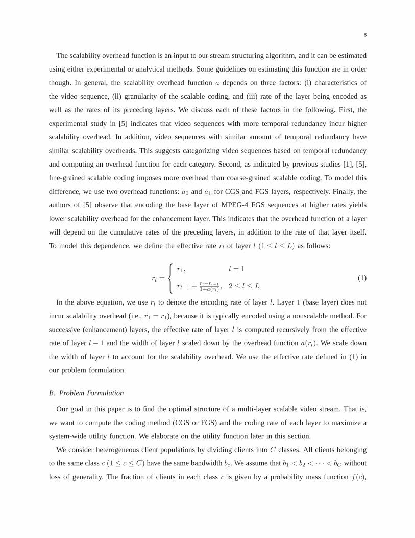
To model this dependence, we define the effective raterl of layer l (1 ≤ l ≤ L) as follows:

rl =

r1, l = 1

rl−1 + rl−rl−1

1+a(rl), 2 ≤ l ≤ L

(1)

In the above equation, we userl to denote the encoding rate of layerl. Layer 1 (base layer) does not

incur scalability overhead (i.e.,r1 = r1), because it is typically encoded using a nonscalable method. For

successive (enhancement) layers, the effective rate of layer l is computed recursively from the effective

rate of layerl − 1 and the width of layerl scaled down by the overhead functiona(rl). We scale down

the width of layerl to account for the scalability overhead. We use the effective rate defined in (1) in

our problem formulation.

B. Problem Formulation

Our goal in this paper is to find the optimal structure of a multi-layer scalable video stream. That is,

we want to compute the coding method (CGS or FGS) and the coding rate of each layer to maximize a

system-wide utility function. We elaborate on the utility function later in this section.

We consider heterogeneous client populations by dividing clients intoC classes. All clients belonging

to the same classc (1 ≤ c ≤ C) have the same bandwidthbc. We assume thatb1 < b2 < · · · < bC without

loss of generality. The fraction of clients in each classc is given by a probability mass functionf(c),

9

where∑C

c=1 f(c) = 1. No assumptions are made on the number of client classes or onthe probability

function. Without loss of generality, we assume thatbC ≤ rmax , which is a pre-determined maximum

rate of the stream. If otherwise, we combine clients with bandwidth larger thanrmax in a class with

bandwidth equal tormax . We can do that because no matter how large the client bandwidth is, it cannot

receive more than the maximum ratermax .

For client classc, its actual received rate is no larger thanbc. To account for scalability overhead, we

define bc to be the effective rate of client classc, where1 ≤ c ≤ C. bc is a function of the adopted

structuring policy, which is defined asS = {(ri, gi), i = 1, 2, . . . , L}, whereri determines the encoding

rate, andgi decides the granularity for layeri. We setgi = 0 if layer i is CGS-coded, andgi = 1 if it is

FGS-coded. We assumeg1 = 0, because the base (first) layer is typically coded with nonscalable coders,

which do not incur scalability overhead. We usel to denote the highest layer that can be transferred to

client c in its entirety (i.e.,rl ≤ bc ≤ rl+1), we write the effective ratebc as:

bc =

rl, gi = 0

rl + bc−rl

1+a1(rl+1), gi = 1

(2)

The effective rate of classc is equal to that of layerl, if layer l + 1 is CGS-coded. If layerl + 1 is

FGS-coded, the additional ratebc − rl can be received on top ofrl, which contributes to the effective

rate of classc after being scaled down by the FGS overhead functiona1(rl+1).

Our problem can formally be stated as follows. Given a scalable stream that can be structured into

up to L layers, and a large number of clients divided intoC classes with their distribution given by

the probability mass functionf(c), find the optimal structuring policyS∗ = {(r∗i , g∗i ), i = 1, 2, . . . , L}

that yields the maximum system-wide utilityY ∗0 , which is defined as the average client utility over all

classes. Mathematically, we write our problem as:

P0(C, L) : Y ∗0 = max

SY0 =

C∑

k=1

f(k)u(bk, bk) (3a)

s.t. r1 < r2 < · · · < rL; (3b)

g1 = 0; (3c)

gi ∈ {0, 1}, ∀i = 2, 3, . . . , L. (3d)

In the above formulation, the utility of a client is a non-decreasing function of the effective rate

achieved by that client. We use the effective rate in the utility function to account for the scalability

10

overhead. We do not impose any restrictions on the utility function: It can be any arbitrary function that

may, for example, describe utilization of system resources, satisfaction of clients, or a combination of

both. Our algorithm, presented in the next section, works with any user-defined utility function. In the

evaluation section, we use three types of utility functions. These utility functions have been used before in

the literature, and they model various aspects such as the effective rate received by clients, the mismatch

between client bandwidth and received stream rate, and client perceived quality in terms of PSNR.

The optimization problem in (3) has an exponential number of feasible solutions, and exhaustively

trying all of them to find the optimal one is extremely expensive. In the next subsection, we propose an

efficient, yet optimal, algorithm to solve it. Our algorithm uses a dynamic programming approach.

C. Efficient Algorithm

We first develop a few lemmas to reduce the search space size of our optimization problemP0(C, L).

We define a subproblem for (3) calledP (c, l), where1 ≤ c ≤ C, and1 ≤ l ≤ L. For this subproblem, we

find the optimal structuring policyS∗ = {(r∗i , g∗i ), i = 1, 2, . . . , l} that yields the maximum system-wide

utility Y ∗(c, l). We then solve this problem iteratively by utilizing solutions of smaller subproblems. In

subproblemP (c, l), we assume that the rate of layer1 is higher than the bandwidth of client classc− 1,

and is no larger than the bandwidth of client classc. We also assume that the layer1 is CGS-coded.

Therefore, clients in classc − 1 and below receive nothing and contribute zero system utility. We can

write this subproblem as:

P (c, l) : Y ∗(c, l) = maxS

Y =C

∑

k=c

f(k)u(bk, bk) (4a)

s.t. r1 < r2 < · · · < rl; (4b)

g1 = 0; (4c)

gi ∈ {0, 1}, ∀i = 2, 3, . . . , l; (4d)

bc−1 < r1 ≤ bc. (4e)

In the above subproblem, constraint (4e) enables us to reduce the search space. We incrementally relax

this limitation to derive the optimal solution for the original problemP0(C, L). Solving subproblem

P (c, l) is still hard. For instance, there are too many possible solutions to consider in order to determine

the optimal coding rate for layer1 alone. We present the following two lemmas to reduce the search

space of the optimal structure policy.

11

Lemma 1:For any given subproblemP (c, l), there exists at lest one optimal solutionS∗ = {(r∗i , g∗i ), i =

1, 2, . . . l} that has the following property:bc−1 < r∗1 ≤ bc < r∗2.

Proof: Let S = {(ri, gi), i = 1, 2, . . . , l} be an optimal structuring policy ofP (c, l), with two or

more layers coded at rates in(bc−1, bc]. Without loss of generality, we assume that there are two layers

coded in this interval, i.e.,bc−1 < r1 < r2 ≤ bc. The cases with more than two layers coded in(bc−1, bc]

can be proved with the same technique. WhenS is employed, following Eq. (1), the clients in classes

c and above receive the effective rater1 + r2−r1

1+a(r2)from layers1 and 2. We notice that, if we were to

adopt a structuring policyS∗ = {(r∗i , g∗i ), i = 1, 2, . . . , l − 1}, where(r∗i , g

∗i ) = (ri+1, gi+1), we still get

optimal performance. This is because: (i) employingS∗ allows clients in classesc and above to receive at

the effective rater∗1 = r2, which is higher than the effective rate achieved byS as the overhead function

is non-negative, and (ii) clients in classesc − 1 and below receive at the same effective rate regardless

of whetherS or S∗ is employed. Thus, employing the structuring policyS∗ achieves at least the same

utility as S, because utility is a non-decreasing function.

Lemma 1 states that if there is an optimal solution that has twoor more layers between two adjacent

classesbc−1 andbc, we can find another optimal solution with only one layer between these two classes.

Therefore, we do not need to allocate two layers between adjacent classes, which reduces the search

space. The following lemma further reduces the search space.

Lemma 2:There exists at least one optimal solution for the subproblemP (c, l) with layer 1 coded at

ratebc. That is, at least one optimal solution has the following property: bc−1 < r∗1 = bc.

Proof: Let S = {(ri, gi), i = 1, 2, . . . , l} be an optimal structuring policy ofP (c, l), wherebc−1 <

r1 < bc. We notice that settingr1 = bc still produces an optimal structuring. This is because the utilities

of clients in classesc− 1 and below are not affected, and the clients in classc and above would achieve

at least the same utility because utility is a non-decreasing function in terms of effective rate.

These two lemmas state that to determiner∗1 for an optimal solution of subproblemP (c, l), we only

need to considerr1 = bc. Next, we consider rates and granularity for other layers for an optimal solution

of subproblemP (c, l). We do so by recursively solving subproblemP (i, l−1), wherec+1 ≤ i ≤ C−l+1.

We present a simple example with three layers and five client classes to demonstrate the basic idea of

our algorithm. The example is shown in Fig. 3. We take subproblem P (2, 2) as example, which finds the

optimal 2-layer structuring policy, where all layers are coded at rates higher thanb1. From the previous

lemmas, we know that settingr1 = b2 would result in an optimal solution. The subproblemP (2, 2) is

then reduced to find the best coding rate and granularity for layer 2, which can be determined from

subproblemsP (3, 1), P (4, 1), andP (5, 1). These three subproblems assume that the rate of layer 2 is

12

l

P (1, 1)

P (4, 2)

1

P (4, 1)

2 P (2, 2)

P (3, 1)3

4

P (2, 1)

P (5, 2)

2

P (5, 1)

c 1

P (3, 2)

P (4, 3)

L = 3

C = 5

P (3, 3)

P (1, 3)

P (2, 3)

P (5, 3)

P (1, 2)

Fig. 3. The optimal structuring problem withC client classes andL layers can be solved using dynamic programming by

dividing it into subproblems. Each problem is solved based on the results of preceding subproblems. Note that, Lemma 1 enables

us to skip subproblems in the lower right part.

in intervals (b2, b3], (b3, b4], and (b4, b5], respectively. This indeed covers all possible rates for layer 2

because we knowr1 < r2. To decide whether layer 2 should be FGS- or CGS-coded, we need toevaluate

the system-wide utility for both cases, and take the maximumof them. Computing the system-wide utility

for each of these smaller subproblems and coding granularity leads to the optimal solution for subproblem

P (2, 2).

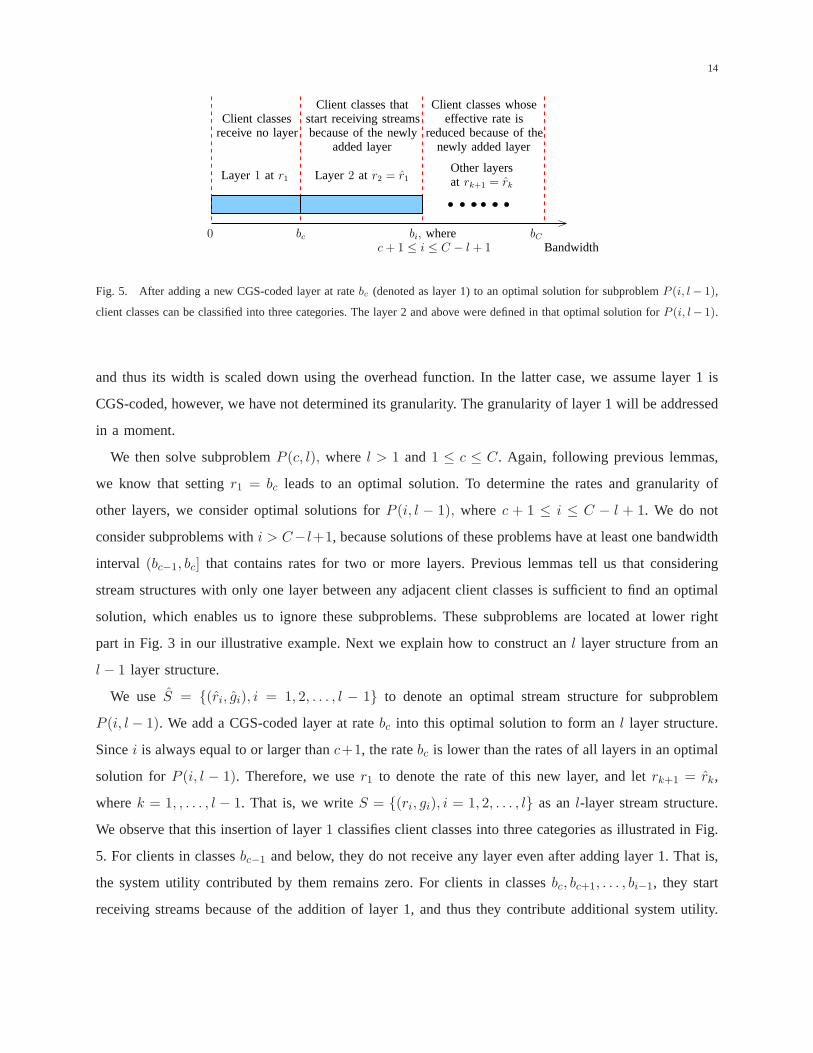
This example reveals that solvingl layer subproblems requires optimal solutions forl − 1 layer

subproblems. Therefore, we sequentially solve subproblemswith 1 layer,2 layers, untilL layers. Notice

that, we assign rates and granularity in descending order. That is, we first determine the optimal rate and

granularity for layerL by solving subproblemP (c, 1), where1 ≤ c ≤ C. We then recursively search for

the optimal rates and granularity for layersL − 1, L − 2, . . . , 1.

We present the details on solving a general subproblemP (c, l), where1 ≤ c ≤ C and1 ≤ l ≤ L as

follows. We first solve subproblemP (c, 1) for 1 ≤ c ≤ C. Previous lemmas tell us that settingr1 = bc

in P (c, 1) leads to an optimal solution. As layer 1 is CGS-encoded, clients in classc − 1 and below

receive nothing, and clients in classc and above receive layer 1, we compute the optimal system utility

Y ∗(c, 1) as:

Y ∗(c, 1) =

∑Ck=c bcf(k), L = 1

∑Ck=c

bc

1+a0(bc)f(k), L 6= 1.

(5)

In the above equation, the first line represents the case wherelayer 1 is indeed the base layer that

has zero scalability overhead. The second line represents the case where layer 1 is not a base layer,

13

Algorithm ScsOpt

1. /*Solve subproblemP (c, 1) for all 1 ≤ c ≤ C.*/

2. for c = 1 to C {

3. Computey(c, 1) using Eq. (5); g(c, 1) = 0; r(c, 1) = bc;

4. }

5. /*Solve subproblemP (c, l) for 2 ≤ l ≤ L, 1 ≤ c ≤ C − l + 1*/

6. for l = 2 to L {

7. for c = l to C − l + 1 {

8. y(c, l) = −∞;

9. /*ComputeY ∗(c, l) using Eq. (8) and solutions of previous subproblemsP (i, l − 1)*/

10. for i = c + 1 to C − l + 1 {

11. Computeutil cgs = Y ∗(i, l − 1) using Eqs. (6-8) withg2 = 0;

12. Computeutil fgs = Y ∗(i, l − 1) using Eqs. (6-8) withg2 = 1;

13. /*Compare utility against known optimum*/

14. if util cgs > y(c, l) {

15. y(c, l) = util cgs; r(c, l) = bc; g(c, l) = 0; n(c, l) = i;

16. }

17. if util fgs > y(c, l) {

18. y(c, l) = util fgs; r(c, l) = bc; g(c, l) = 1; n(c, l) = i;

19. }

20. }

21. }

22. }

23. /*Find the optimal structuring forP0(C, L)*/

24. prev layer = argmax1≤c≤C−L+1

y(c, L);

25. /*Find r∗l andg∗l for all l using backtracking*/

26. g∗1 = 0;

27. for l = L to 1 {

28. r∗L−l+1 = r(prev layer , l); g∗L−l+2 = g(prev layer , l);

29. prev layer = n(prev layer, l);

30. }

31. r∗L = r(prev layer , 1);

Fig. 4. The proposed algorithm to compute the optimal structure of scalablestreams.

14

Bandwidthbi, where

c + 1 ≤ i ≤ C − l + 1

Client classesreceive no layer

Client classes thatstart receiving streamsbecause of the newly

added layer

Client classes whoseeffective rate is

reduced because of thenewly added layer

Other layersat rk+1 = rk

Layer 1 at r1 Layer 2 at r2 = r1

0 bCbc

Fig. 5. After adding a new CGS-coded layer at ratebc (denoted as layer 1) to an optimal solution for subproblemP (i, l− 1),

client classes can be classified into three categories. The layer 2 and above were defined in that optimal solution forP (i, l− 1).

and thus its width is scaled down using the overhead function. In the latter case, we assume layer 1 is

CGS-coded, however, we have not determined its granularity.The granularity of layer 1 will be addressed

in a moment.

We then solve subproblemP (c, l), where l > 1 and 1 ≤ c ≤ C. Again, following previous lemmas,

we know that settingr1 = bc leads to an optimal solution. To determine the rates and granularity of

other layers, we consider optimal solutions forP (i, l − 1), wherec + 1 ≤ i ≤ C − l + 1. We do not

consider subproblems withi > C−l+1, because solutions of these problems have at least one bandwidth

interval (bc−1, bc] that contains rates for two or more layers. Previous lemmas tell us that considering

stream structures with only one layer between any adjacent client classes is sufficient to find an optimal

solution, which enables us to ignore these subproblems. These subproblems are located at lower right

part in Fig. 3 in our illustrative example. Next we explain howto construct anl layer structure from an

l − 1 layer structure.

We use S = {(ri, gi), i = 1, 2, . . . , l − 1} to denote an optimal stream structure for subproblem

P (i, l − 1). We add a CGS-coded layer at ratebc into this optimal solution to form anl layer structure.

Sincei is always equal to or larger thanc+1, the ratebc is lower than the rates of all layers in an optimal

solution for P (i, l − 1). Therefore, we user1 to denote the rate of this new layer, and letrk+1 = rk,

wherek = 1, , . . . , l − 1. That is, we writeS = {(ri, gi), i = 1, 2, . . . , l} as anl-layer stream structure.

We observe that this insertion of layer1 classifies client classes into three categories as illustrated in Fig.

5. For clients in classesbc−1 and below, they do not receive any layer even after adding layer 1. That is,

the system utility contributed by them remains zero. For clients in classesbc, bc+1, . . . , bi−1, they start

receiving streams because of the addition of layer 1, and thus they contribute additional system utility.

15

We define this additional system utility as functionU(c, l, i), which is given as:

U(c, l, i) =

bc

∑i−1k=c f(k), l = L, g2 = 0

∑i−1k=c[bc + bk−bc

1+a1(bi)]f(k), l = L, g2 = 1

bc

1+a0(bc)

∑i−1k=c f(k), l 6= L, g2 = 0

∑i−1k=c[

bc

1+a0(bc)+ bk−bc

1+a1(bi)]f(k), l 6= L, g2 = 1.

(6)

The above equation indicates that the additional system utility depends on the granularity of layer 2.

The first two lines consider that layer 1 is the base layer that has no scalability overhead, while the other

two lines assume layer 1 is CGS-coded. For clients in classbi and above, they receive layer 2 before and

after the addition of layer 1. Their effective rates, however, are reduced because of the addition of layer

1 as scalability overhead is a non-increasing function. We define the effective rate reduction as function

D(c, l, i), which is given as:

D(c, l, i) =

bi

1+a0(bi)− bc −

bi−bc

1+a0(bi), l = L, g2 = 0

bi

1+a0(bi)− bc −

bi−bc

1+a1(bi), l = L, g2 = 1

bi

1+a0(bi)− bc

1+a0(bc)− bi−bc

1+a0(bi), l 6= L, g2 = 0

bi

1+a0(bi)− bc

1+a0(bc)− bi−bc

1+a1(bi), l 6= L, g2 = 1.

(7)

The above equation follows the definition of effective rates. The first term represents the effective rate

for these clients before the addition of layer 1. The second and third terms account for the effective rate

after layer 1 is added. Again, the effective rate reduction depends on the granularity of layer 2.

The analysis of these categories of client classes allows us to compute the system-wide utility after

adding a CGS-coded layer to the optimal structure of subproblem P (i, l− 1). Therefore, we can use the

following formulation to solve subproblemP (c, l) by utilizing optimal solutions for smaller subproblems:

Y ∗(c, l) = maxc+1≤i≤C−l+1,

g2∈{1,0}

{

Y ∗(i, l − 1) − D(c, l, i)C

∑

k=i

f(k) + U(c, l, i)

}

, (8)

whereY ∗(c, l) represents the optimal system utility for subproblemP (c, l).

The formulation in (8) updates the maximal system utility ofP (i, l− 1) by deducting utilityD(c, l, i)

from all clients in classi and above, and adding the additional utility functionU(c, l, i). It finds the

subproblemP (i, l− 1) and the granularityg2 that maximize system-wide utility for subproblemP (c, l).

Notice that,g2 represents the granularity of the lowest layer for subproblemP (i, l−1). g2 was assumed to

16

be CGS-coded in subproblemP (i, l−1), and its optimal setting is determined when solving subproblem

P (c, l) using (8). An important property of (8) is that we effectively consider all possible combinations

of r1 and g2. Therefore, we can use dynamic programming technique to optimally solve subproblem

P (c, l) for its optimal structure. The following theorem shows how toconstruct an optimal solution for

problemP0(C, L) based on optimal solutions for subproblemsP (c, l).

Theorem 1 (Optimality):Let S∗(c, l) denote the optimall-layer structure for subproblemP (c, l) that

achieves the maximal system utilityY ∗(c, l). The optimal structureS∗ for the original problemP0(C, L)

is the one that achieves maximum system utility:Y ∗0 = max1≤c≤C−L+1{Y

∗(c, L)}.

Proof: Let S∗ be an optimal structure for problemP0(C, L), and r∗1 represent the coding rate of

layer1 in S∗. Clearly, we haver∗1 ∈ [0, bC ]. This is becauser∗1 can not be larger thanbC , otherwise none

of the client classes receives anything, and thusS∗ can not be an optimal structure. We divide the range

[0, bC ] into non-overlapping intervals(bc−1, bc], wherec = 1, 2, . . . , C andb0 = 0. Now assume that the

optimal rater∗1 occurs in an arbitrary interval(bz−1, bz], for some1 ≤ z ≤ C. Because the constraint

bz−1 < r∗1 ≤ bz is satisfied, we know that the optimal structure for subproblem P (z, L) leads to the

maximum system wide utility for problemP0(C, L). As r∗1 must fall in exactly one of these intervals,

we solve subproblemsP (c, L), for c = 1, 2, . . . , C, then compute theY ∗0 by: Y ∗

0 = max1≤c≤C

{Y ∗(c, L)},

which results in the maximal system utilityY ∗0 for the original problemP0(C, L). Furthermore, Lemma

1 allows us to ignore subproblemsP (c, L), wherec = C − L + 2, C − L + 3, . . . , C.

The above theorem illustrates that the optimal structure forproblem P0(C, L) can be derived by

finding the maximal system-wide utility among all optimal solutions for subproblemsP (c, L), where

1 ≤ c ≤ C − L + 1, while the optimal solutions for subproblemsP (c, L) can be found by iteratively

solving smaller subproblems. Next, we present the details of our algorithm.

The pseudo-code of our algorithm is shown in Fig. 4. The algorithm takes the following inputs: client

class distributionfc, client network bandwidthbc, and number of layersL. The algorithm also requires

specifying the utility function and the scalability overhead function. It produces the optimal rater∗l and

granularityg∗l (CGS or FGS) for each layerl. The algorithm works by sequentially solving subproblems

P (c, l) for 1 ≤ l ≤ L and 1 ≤ c ≤ C. It re-uses the optimal solutions of(l − 1)-layer structuring

subproblems to find thel-layer optimal solutions. We first solve the1-layer structuring subproblem in

lines 2—4. We then solve all other subproblems with more thanone layer. We do this by using the two

for loops starting at lines 6 and 7, which go through layers and client classes, respectively. We solve

subproblemP (c, l) as follows. The loop in lines 10—20 takes an optimall− 1 layer structure produced

by previous subproblemsP (i, l − 1), adds a layer to it, and computes the system-wide utility of this

17

0 500 1000 14000

0.005

0.01

0.015

0.02

0.025

0.03

0.035

Client class bandwidth (kbps)

Distr

ibution

(a) Scenario II: bi-modal (skewed to the

right)

0 500 1000 14000

0.02

0.04

0.06

0.08

0.1

0.12

Client class bandwidth (kbps)

Distr

ibution

(b) Scenario III: bi-modal (skewed to the

left)

0 500 1000 1500 2000 25000

0.02

0.04

0.06

0.08

Client class bandwidth (kbps)

Distr

ibution

(c) Scenario IV: Internet distribution

Fig. 6. Three of the client bandwidth distributions considered in the experimental study. The fourth (uniform distribution) is

not shown.

new l-layer structuring policy. To determine the optimal granularity, it computes a CGS-coded utility in

line 11 and an FGS-coded utility in line 12. In lines 14—19, we check whether the currenti leads to a

structuring policy with higher system-wide utility than the best knownl-layer structure. In line 24, we

find the optimal structuring policy for problemP0(C, L) based on the solutions for subproblems using

Theorem 1. Finally, lines 26—31 find the optimalL-layer stream structure using backtracking technique.

The following theorem gives the time and space complexities of our algorithm.

Theorem 2 (Complexity):The time complexity of the ScsOpt algorithm in Fig. 4 isO(C3L) and its

space complexity isO(CL), whereC is the number of client classes andL is the number of layers in

the video stream.

Proof: The algorithm uses two for-loops to sequentially solve subproblemP (c, l), which takeO(CL).

For eachP (c, l), we checkC− l+1 previous subproblems, which takes anotherO(C). For each previous

subproblem, we compute its system-wide utility inO(C) steps. Therefore, the time complexity of our

algorithm isO(C3L). It is easy to see that the space complexity for our algorithmis O(CL), because the

data structures used are:y(c, l) for storing optimal system utility;r(c, l) for storing optimal rate;g(c, l)

for storing optimal granularity; andn(r, l) for back-tracking. All these data structures are 2-dimensional

arrays, where1 ≤ c ≤ C, and1 ≤ l ≤ L.

V. EVALUATION

In this section, we first describe our experimental setup. Thenwe verify the optimality of our algorithm

by comparing it against an exhaustive search algorithm. We then demonstrate that our algorithm allows

18

various utility functions and produces optimal stream structures. That is followed by a study on the impact

of choosing different utility functions. Next, we compare our algorithm with a widely used heuristic stream

structuring algorithm. Last, we report the running time of our algorithm.

A. Setup

As mentioned in Section II, our algorithm would be run by a streaming server receiving requests from

many concurrent clients for a specific scalable stream. The clients are heterogeneous in bandwidth. The

server uses our algorithm and the client bandwidth information to determine the optimal structure of the

stream. The output of our algorithm is the encoding rate and granularity (FGS or CGS) of each layer.

This information is then fed to a video encoder such as H.264/SVC. We have implemented our algorithm

in Java, and to rigorously evaluate its performance we: (i) consider three different utility functions to

quantify the optimal solution, and (ii) we simulate a large number of clients with different realistic

bandwidth distributions. We elaborate on these parametersin the following.

Our algorithm works with any utility functionu(bc, bc), wherebc is the effective rate of the received

stream, andbc is the available bandwidth of clientc. Three utility functions are employed in our

experiments: (i)urate(bc, bc) = bc, which assumes that the higher the effective rate that a client receives,

the more satisfied that client will be; (ii)uutilization(bc, bc) = bc/bc, which tries to match the rate received

by a client with its bandwidth; and (iii)upsnr which maximizes the client-perceived quality (in PSNR)

by using rate-distortion (R-D) curves to map the effective rate to perceived quality. For constructing

R-D curves, we adopt a recent H.264/AVC R-D function which assumes that the transform coefficients

are Cauchy distributed [23]. The R-D function is given as:D = cR−γ , where the distortionD is in

mean-square error (MSE) and rateR is in bits per pixel. The model parametersc and γ are sequence

dependents. The authors of [23] show that this model is more accurate than Laplacian and Gaussian based

R-D models. We choseupsnr (bc, bc) = −10 log10[15.3787(0.1184bc)−2.2] in our experiments with CIF

video sequences. We note that this R-D model is proposed for nonscalable H.264/AVC coded streams. It

is, however, applicable in our experiments because we convert actual rates to effective rates, which are

equivalent to the rates of nonscalable stream.

We consider100, 000 clients with network bandwidth distributed according to four representative

distributions. Fig. 6 shows three of these distributions. Thefirst distribution (not shown in the figure) is

uniform between35 and3005 kbps. The second is a bi-modal distribution that consists of two normally-

distributed peaks with means at250 kbps and1000 kbps, and standard deviations of25 and 100. This

bi-modal distribution is skewed to the right:80% of client classes are from the normal distribution with

19

mean1000 kbps. The third is a bi-modal distribution with the same setting, except that it is skewed to

the left: 80% of client classes are from the normal distribution with mean250 kbps. The fourth is a

multi-modal distribution with three normal distributions, which represents a typical client distribution in

today’s Internet:50% of clients are equipped with dial-up connections, which have a normal distribution

with mean40 kbps and standard deviation of25 kbps; 35% of clients use DSL services, where the

average bandwidth is1000 kbps with standard deviation of100 kbps; and15% of clients have high-

speed connections with average bandwidth2000 kbps and standard deviation of200 kbps.

Finally, our algorithm can employ various user-specified scalability overhead functions. Previous studies

[1], [5] reveal that FGS coded layers results in higher scalability overhead compared to CGS coded layers.

Therefore, we definea0(rl) and a1(rl) for CGS and FGS overhead function, wherea0(rl) ≤ a1(rl) at

any layer raterl. In our experiments, we leta0(0) = 5% anda1(0) = 20%. We let both CGS and FGS

overhead reach zero whenrl ≥ 5000 kbps. That is, we have the following scalability overhead functions:

a0(rl) = max{0.05 − 0.00001rl, 0}, anda1(rl) = max{0.20 − 0.00004rl, 0}.

B. Optimality of our Algorithm

We compare the stream structures resulted by our algorithm against optimal solutions derived by an

exhaustive search algorithm. We can only cover a few layers using exhaustive search approach due to the

huge search space. We search for up to4 layers optimal coding structures. We stop at4-layer, because the

exhaustive search algorithm did not terminate in several hours for more layers. Fig. 7 shows the system-

wide utility achieved by our algorithm and by the exhaustivesearch algorithm for all four scenarios and

all considered utility functions. This figure clearly confirms the optimality of our algorithm.

C. Optimal Stream Structuring

Our algorithm takes client bandwidth distribution as input. It produces a stream structure that results

in the highest utility. As mentioned above, we use three different utility functions in our experiments.

These utility functions lead to different optimal stream structures. Fig. 8 shows the optimal stream

structuring policies computed by our algorithm for 5-layerscalable stream in scenario IV with different

utility functions. We see that the resulted stream structure is influenced by the chosen utility function.

Specifically, the following stream structures are determinedto be the optimal stream structure for each

of the utility functions: (i)urate : {(735, CGS), (805, CGS), (855, CGS), (885, CGS), (2745, FGS)}, (ii)

uutilization : {(5, CGS), (15, CGS), (25, CGS), (35, CGS), (2745, FGS)}, and (iii) upsnr : {(35, CGS),

20

1 2 3 4 1 2 3 4 1 2 3 4 1 2 3 40

500

1000

1500

Number of layers

Ave

rage

effec

tive

rate

(kbps)

ScsOptOpt

I

II

III

IV

︷ ︸︸ ︷

︷ ︸︸ ︷

︷ ︸︸ ︷

︷ ︸︸ ︷

(a) All scenarios withurate utility

1 2 3 4 1 2 3 4 1 2 3 4 1 2 3 40

0.2

0.4

0.6

0.8

1

Number of layers

Ave

rage

utiliza

tion

ScsOptOpt

︷ ︸︸ ︷ ︷ ︸︸ ︷ ︷ ︸︸ ︷ ︷ ︸︸ ︷

I II III IV

(b) All scenarios withuutilization utility

1 2 3 4 1 2 3 4 1 2 3 4 1 2 3 40

10

20

30

40

Number of layers

Ave

rage

quality

inPSN

R(d

B)

ScsOptOpt

︷ ︸︸ ︷I

︷ ︸︸ ︷

︷ ︸︸ ︷

︷ ︸︸ ︷

II

IIIIV

(c) All scenarios withupsnr utility

Fig. 7. Comparison between our algorithm (ScsOpt) and the optimal solution(Opt) derived by an exhaustive search algorithm

for three different utility functions. Results for scenarios I, II, III, and IV are shown from left to right.

(45, CGS), (95, FGS), (685, CGS), (2745, FGS)}. Elements in each 2-tuple represent coding rate in kbps

and granularity, respectively.

These results show that our algorithm is general and can be used with various utility functions in

different environments. In the next subsection, we providesome guidelines on choosing the appropriate

utility function.

D. Choosing Utility Functions

In this section, we shed some lights on the impact of using oneutility function versus another. We

do so by searching optimal stream structures for various scenarios and different number of layers. We

show a sample result of constructing an optimal4-layer stream structure for scenario IV as follows. In

21

0 500 1000 1500 2000 25000

0.05

0.1

Client class bandwidth (kbps)D

istr

ibution

urate

uutilization

upsnr

Fig. 8. Optimal structuring of a scalable video stream with5 layers for scenario IV produced by our optimal algorithm with

different utility functions.

500 1000 1500 2000 2500 30000

5

10

15

Client class bandwidth (kbps)

Cla

sseff

ective

rate

(a) Effective rate

500 1000 1500 2000 2500 30000

0.02

0.04

0.06

0.08

Client class bandwidth (kbps)

Cla

ssbandw

idth

utiliza

tion

(b) Bandwidth utilization

500 1000 1500 2000 2500 30000

0.1

0.2

0.3

0.4

0.5

Client class bandwidth (kbps)

Cla

ssquality

(c) Perceived quality

Fig. 9. Utility achieved by individual classes using our algorithm with variousutility functions.

scenario IV,50% of the clients have narrowband dial-up service,35% have DSL service, and15% have

higher speed. Our algorithm produces the following stream structures for each utility function: (i)urate :

{(735, CGS), (805, CGS), (855, CGS), (2745, FGS)}, (ii) uutilization : {(5, CGS), (15, CGS), (25, CGS),

(2745, FGS)}, and (iii) upsnr : {(25, CGS), (35, CGS), (45, CGS), (2745, FGS)}.

We plot the utility of individual classes in Fig. 9. The utilityis derived by multiplying the client utility

by the fraction of clients in that class. We first notice that the effective rate function favors broadband

clients as indicated by Fig. 9(a). Actually the dial-up clients are completely ignored, as the first layer

22

rate is set at735 kbps. This is because a satisfied broadband client results in much higher effective

rate compared to a satisfied narrowband client. In addition, increasing layer coding rates leads to lower

scalability overhead thus higher effective rates. Consequently, narrowband clients are sacrificed. This

poses a fairness issue among clients.

Using the bandwidth utilization function results in a fair stream structure as indicated by Fig. 9(b).

This is because we use a relative utility function, in which the decision is not biased by the value of

client bandwidth. Rather, the decision is made based on the mismatch between the client bandwidth and

the receiving rate. We also observe a quite fair stream structure in Fig. 9(c). More resources are allocated

to narrowband clients, compared to the effective rate case,because of the non-linear R-D curve shape.

The R-D curve increases dramatically at low rates, but saturates at high rates. Therefore, to maximize

system-wide utility, more resources are allocated to clients that are receiving at lower rates.

These results help content providers to choose a utility function that suit their needs. For instance,

a content provider would use the effective rate utility function if its customers are charged in terms

of traffic amount. A non-profit organization may be more interested in inter-client fairness and chooses

bandwidth utilization function. Another content providerwho wants to boost its client satisfaction would

adopt the perceived quality function, which accommodates the non-linear relationship between rate and

actual perceived quality.

E. Comparison with Previous Structuring Algorithm

We compare the stream structures resulted by our algorithm against the heuristic structuring algorithm

used in [15], [16]. This heuristic algorithm takes two rates for minimum and maximum supported decoding

rates. It uses these two rates to code the first and the last layers, and then exponentially allocates rates for

intermediate layers. That is, a layerl is assigned raterminρl−1, wherermin andrmax are the minimum

and maximum supported rates. The factorρ is given byL−1√

rmax/rmin , whereL is the total number of

layers. We usermin = 50 kbps andrmax = 1500 kbps in our experiments. This covers a wide range

of clients, from dial-up to broadband access links. We denote this algorithm by Expo in the plots. Figs

10-12 illustrate the achieved system-wide utility by ScsOptand Expo algorithms. These figures indicate

that our algorithm outperforms the heuristic algorithm with significant margins in all cases.

We note that Expo is the only algorithm we could find in the literature that may be applied to our

stream structuring problem. Moreover, if there were other algorithms, the best they can do is to achieve

results similar to our algorithm, because our algorithm is optimal as shown in Sec. IV-C and verified in

Sec. V-C.

23

1 2 3 4 5 6 7 80

500

1000

1500

Number of layers

Ave

rage

effec

tive

rate

(kbps)

ScsOptExpo

(a) Scenario I

1 2 3 4 5 6 7 80

200

400

600

800

1000

Number of layers

Ave

rage

effec

tive

rate

(kbps)

ScsOptExpo

(b) Scenario II

1 2 3 4 5 6 7 80

100

200

300

400

Number of layers

Ave

rage

effec

tive

rate

(kbps)

ScsOptExpo

(c) Scenario III

1 2 3 4 5 6 7 80

200

400

600

800

Number of layers

Ave

rage

effec

tive

rate

(kbps)

ScsOptExpo

(d) Scenario IV

Fig. 10. Comparison between our algorithm (ScsOpt) and the heuristic algorithm (Expo) that exponentially allocates rates to

layers. Data shown for using effective rate as utility function.

F. Running Time

While heuristic algorithms are typically efficient, they do not lead to optimal structuring policies. For

example, the Expo algorithm produces significantly lower system-wide utility compared to our optimal

algorithm. Therefore, we do not report the running time of heuristic algorithms.

Because of the huge search space, the exhaustive search algorithm consumes tremendous computational

resources. For a moderate size problem with100 client classes and4 layers, the exhaustive search

algorithm took at least30 minutes to terminate. The running time is even longer if a complicated

utility function—e.g., the perceived quality function—isemployed. Consequently, the exhaustive search

algorithm is not practical.

24

1 2 3 4 5 6 7 80

0.2

0.4

0.6

0.8

1

Number of layers

Ave

rage

bandw

idth

utiliza

tion

ScsOptExpo

(a) Scenario I

1 2 3 4 5 6 7 80

0.2

0.4

0.6

0.8

1

Number of layers

Ave

rage

bandw

idth

utiliza

tion

ScsOptExpo

(b) Scenario II

1 2 3 4 5 6 7 80

0.2

0.4

0.6

0.8

1

Number of layers

Ave

rage

bandw

idth

utiliza

tion

ScsOptExpo

(c) Scenario III

1 2 3 4 5 6 7 80

0.2

0.4

0.6

0.8

1

Number of layers

Ave

rage

bandw

idth

utiliza

tion

ScsOptExpo

(d) Scenario IV

Fig. 11. Comparison between our algorithm (ScsOpt) and the heuristic algorithm (Expo) that exponentially allocates rates to

layers. Data shown for using bandwidth utilization as utility function.

We present the running time of our algorithm in Table I. Our algorithm terminates in negligible time

for straightforward utility functions: effective rate andbandwidth utilization. For instance, when using

urate as utility function, our algorithm solves a problem with more than 200 client classes and 8 layers

in less than one second. In addition, our algorithm terminates in a few seconds even with a complicated

perceived quality function. For example, our algorithm takes up to 2.5 seconds to solve a problem with

100 client class and up to 8 layers. Because of its low computational complexity, using our algorithm with

more complex utility functions is feasible and practical. For instance, our algorithm can adopt an elaborate

R-D function for higher estimation accuracy, and thus results in higher average perceived quality.

25

1 2 3 4 5 6 7 80

10

20

30

40

Number of layers

Ave

rage

quality

inPSN

R(d

B)

ScsOptExpo

(a) Scenario I

1 2 3 4 5 6 7 80

10

20

30

40

Number of layers

Ave

rage

quality

inPSN

R(d

B)

ScsOptExpo

(b) Scenario II

1 2 3 4 5 6 7 80

5

10

15

20

25

30

Number of layers

Ave

rage

quality

inPSN

R(d

B)

ScsOptExpo

(c) Scenario III

1 2 3 4 5 6 7 80

5

10

15

20

25

Number of layers

Ave

rage

quality

inPSN

R(d

B)

ScsOptExpo

(d) Scenario IV

Fig. 12. Comparison between our algorithm (ScsOpt) and the heuristic algorithm (Expo) that exponentially allocates rates to

layers. Data shown for using perceived quality as utility function.

VI. CONCLUSION

We have formulated an optimization problem to determine theoptimal rate and encoding granularity

(CGS or FGS) of each layer in a scalable video stream that maximizes a system-defined utility function

for a given client distribution. We have proposed an optimalalgorithm to solve this problem. efficient

and runs inO(C3L), whereL is the number of layers in the video stream andC is the number of

client classes. SinceL andC are typically small integers, our algorithm is computationally efficient. Our

algorithm is Our algorithm can employ arbitrary utility functions for clients. To demonstrate the generality

of our algorithm, we used three utility functions in our experimental study. These utility functions have

been used before in the literature, and they model various performance metrics such as the effective rate

26

TABLE I

RUNNING TIME (IN msec) OF OUR ALGORITHM WITH ALL CONSIDERED TEST SCENARIOS.

Test No. of No. of layersL

scenario classesC 1 2 3 4 5 6 7 8

Using urate as utility function

I 100 4 174 134 221 272 331 250 349

II 102 4 181 265 198 398 174 230 259

III 99 3 127 223 209 150 232 287 182

IV 222 16 230 326 397 506 755 857 741

Using uutilization as utility function

I 100 4 150 136 168 209 204 395 236

II 102 4 141 260 293 259 214 314 225

III 99 4 146 166 208 445 198 188 362

IV 222 9 273 448 498 656 660 886 854

Using upsnr as utility function

I 100 7 309 650 994 1306 1631 1959 2426

II 102 8 449 867 1083 1430 1829 2104 2456

III 99 7 313 664 1017 1285 1579 1919 2220

IV 222 28 2547 6305 9722 13197 16768 20325 24935

received by clients, the mismatch between client bandwidthand received stream rate, and the client-

perceived quality in terms of PSNR. We experimentally verified that our algorithm produces the optimal

results and runs in a few seconds on a commodity PC. We also compared our algorithm against another

algorithm that has been used before in the literature, and weshowed that our algorithm outperforms the

other one in all cases.

We studied the effect of various structuring of scalable video streams on client utilities for different

utility functions. By analyzing various utility functions, we provided guidelines for content providers to

choose the appropriate utility function that suits their needs. For instance, a content provider can use the

effective rate as a utility function if its customers are charged in terms of traffic amount. A non-profit

organization may be more interested in inter-client fairness and chooses a utility function based on the

mismatch between client bandwidth and received rate.

27

ACKNOWLEDGMENT

This work is partially supported by the Natural Sciences and Engineering Research Council (NSERC)

of Canada under Discovery Grant #313083 and RTI Grant #344619.

REFERENCES

[1] H. Schwarz, D. Marpe, and T. Wiegand, “The scalable H.264/MPEG4-AVC extension: Technology and applications,” in

European Symposium on Mobile Media Delivery (EuMob’06), Sardinia, Italy, September 2006.

[2] Joint Video Team, “Joint scalable video model reference software,” JSVM 8.0, February 2007.

[3] H. Radha, M. van der Schaar, and Y. Chen, “The MPEG-4 fine-grained scalable video coding method for multimedia

streaming over IP,”IEEE Transactions on Multimedia, vol. 3, no. 1, pp. 53–68, March 2001.

[4] W. Li, “Overview of fine granularity scalability in MPEG-4 video standard,” IEEE Transactions on Circuits and Systems

for Video Technology, vol. 11, no. 3, pp. 301–317, March 2001.

[5] M. van der Schaar and H. Radha, “Adaptive motion-compensationfine-granular-scalability (AMC-FGS) for wireless video,”

IEEE Transactions on Circuits and Systems for Video Technology, vol. 12, no. 6, pp. 32–51, June 2002.

[6] J. Liu, B. Li, and Y. Zhang, “Adaptive video multicast over the Internet,” IEEE Multimedia Magazine, vol. 10, no. 1, pp.

22–33, January 2003.

[7] X. Li, M. Ammar, and S. Paul, “Video multicast over the Internet,”IEEE Network Magazine, vol. 13, no. 2, pp. 46–60,

March 1999.

[8] S. Cheung, M. Ammar, and X. Li, “On the use of destination set grouping to improve fairness in multicast video

distribution,” in Proc. of IEEE INFOCOM’96, San Francisco, CA, March 1996, pp. 553–560.

[9] S. McCanne, V. Jacobson, and M. Vetterli, “Receiver-driven layered multicast,” inProc. of ACM SIGCOMM’96, Palo Alto,

CA, August 1996, pp. 117–130.

[10] X. Li, S. Paul, and M. Ammar, “Multi-session rate control for layered video multicast,” inProc. of ACM/SPIE Multimedia

Computing and Networking (MMCN’99), San Jose, CA, January 1999, pp. 175–189.

[11] L. Vicisano, L. Rizzo, and J. Crowcroft, “TCP-like congestion control for layered multicast data transfer,” inProc. of IEEE

INFOCOM’98, San Francisco, CA, March 1998, pp. 996–1003.

[12] T. Jiang, M. Ammar, and E. Zegura, “On the use of destination setgrouping to improve inter-receiver fairness for multicast

ABR sessions,” inProc. of IEEE INFOCOM’00, Tel Aviv, Israel, March 2000, pp. 42–51.

[13] N. Shacham, “Multipoint communication by hierarchically encoded data,” in Proc. of IEEE INFOCOM’92, Florence, Italy,

May 1992, pp. 2107–2114.

[14] Y. Yang, M. Kim, and S. Lam, “Optimal partitioning of multicast receivers,” in Proc. of IEEE International Conference

on Network Protocols (ICNP’00), Osaka, Japan, November 2000, pp. 129–140.

[15] J. Liu, B. Li, Y. Hou, and I. Chlamtac, “Dynamic layering and bandwidth allocation for multi-session video broadcasting

with general utility functions,” inProc. of IEEE INFOCOM’03, San Francisco, CA, March 2003, pp. 630–640.

[16] J. Liu, B. Li, and Y. Zhang, “Optimal stream replication for video simulcasting,”IEEE Transactions on Multimedia, vol. 8,

no. 1, pp. 162–169, February 2006.

[17] I. Radulovic, P. Frossard, and O. Verscheure, “Adaptive video streaming in lossy networks: versions or layers?” inProc.

of IEEE International Conference on Multimedia and Expo (ICME’04), Taipei, Taiwan, June 2004, pp. 1915–1918.

28

[18] P. de Cuetos, D. Saparilla, and K. Ross, “Adaptive streaming of stored video in a TCP-friendly context: Multiple versions

or multiple layers?” inProc. of International Packet Video Workshop (PV’01), Kyongju, Korea, April 2001.

[19] T. Kim and M. Ammar, “A comparison of layering and stream replication video multicast schemes,” inProc. of ACM

International Workshop on Network and Operating Systems Support forDigital Audio and Video (NOSSDAV’01), Port

Jefferson, NY, June 2001, pp. 63–72.

[20] ——, “A comparison of heterogeneous video multicast schemes: layered encoding or stream replication,”IEEE Transactions

on Multimedia, vol. 7, no. 6, pp. 1123–1130, December 2005.

[21] M. Dai, D. Loguinov, and H. Radha, “Rate-distortion analysis and quality control in scalable Internet streaming,”IEEE

Transactions on Multimedia, vol. 8, no. 6, pp. 1135–1146, December 2006.

[22] C. Hsu and M. Hefeeda, “Optimal bit allocation for fine-grained scalable video sequences in distributed streaming

environments,” inProc. of ACM/SPIE Multimedia Computing and Networking (MMCN’07), San Jose, CA, January 2007.

[23] N. Kamaci, Y. Altunbasak, and R. Mersereau, “Frame bit allocation for the H.264/AVC video coder via Cauchy-density-

based rate and distortion models,”IEEE Transactions on Circuits and Systems for Video Technology, vol. 15, no. 8, pp.

994–1006, August 2005.