1 Optimization Optimization = transformation that improves the performance of the target code Optimization must not change the output must not cause errors that were not present in the original program must be worth the effort (profiling often helps). Which optimizations are most important depends on the program, but generally, loop optimizations, register allocation and instruction scheduling are the most critical. Local optimizations : within Basic Blocks Superlocal optimizations : within Extended Basic Blocks Global optimizations: within Flow Graph
Transcript
1
Optimization
Optimization = transformation that improves the performance of the target code
Optimization must not change the output must not cause errors that were not present in the
original program must be worth the effort (profiling often helps).
Which optimizations are most important depends on the program, but generally, loop optimizations, register allocation and instruction scheduling are the most critical.
Local optimizations : within Basic Blocks Superlocal optimizations : within Extended Basic Blocks Global optimizations: within Flow Graph
2
Extended Basic Block
An Extended Basic Block is a maximal sequence of instructions beginning with a leader, that contains no join nodes other than its leader.
Some local optimizations are more effective when applied on EBBs. Such optimizations tend to treat the paths through
an EBB as if they were in a single block.
3
Algebraic simplifications
These include: Taking advantage of algebraic identities
(x*1) is x Strength reduction
(x*2) is (x << 1) Simplifications such as
- (- x ) is x (1 || x ) is true (1 && x ) is x *(& x ) is x
4
Constant folding
Definition: The evaluation at compile time of expressions whose
values are known to be constant.
Is it always safe? Booleans: yes Integers: almost always
issues: division by zero, overflow Floating point: usually no
issues: compiler's vs. processor's floating point arithmetic, exceptions, etc.)
May be combined with constant propagation.
5
Redundancy elimination
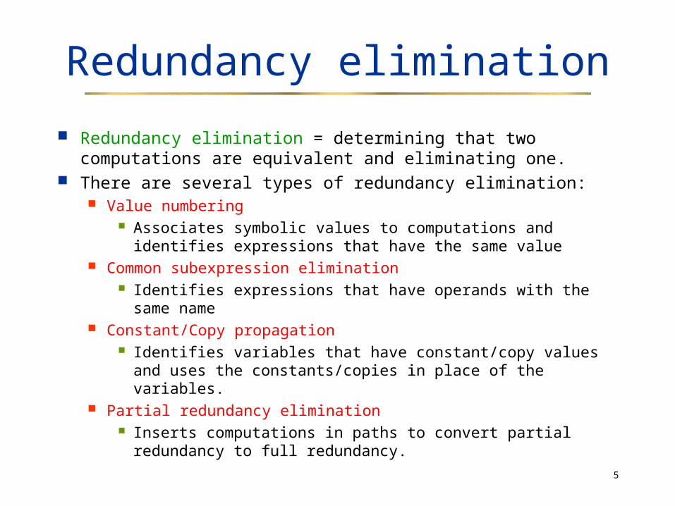
Redundancy elimination = determining that two computations are equivalent and eliminating one.
There are several types of redundancy elimination: Value numbering
Associates symbolic values to computations and identifies expressions that have the same value
Common subexpression elimination Identifies expressions that have operands with the
same name Constant/Copy propagation
Identifies variables that have constant/copy values and uses the constants/copies in place of the variables.
Partial redundancy elimination Inserts computations in paths to convert partial
redundancy to full redundancy.
6
Redundancy elimination
read(i)j = i+1k = in = k+1
i = 2j = i*2k = i+2
a = b * c
x = b * c
7
Value numbering
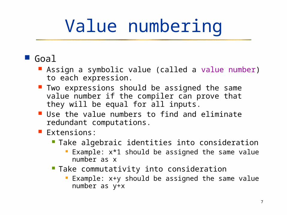
Goal Assign a symbolic value (called a value number) to
each expression. Two expressions should be assigned the same value
number if the compiler can prove that they will be equal for all inputs.
Use the value numbers to find and eliminate redundant computations.
Extensions: Take algebraic identities into consideration
Example: x*1 should be assigned the same value number as x
Take commutativity into consideration Example: x+y should be assigned the same value
number as y+x
8
Value numbering
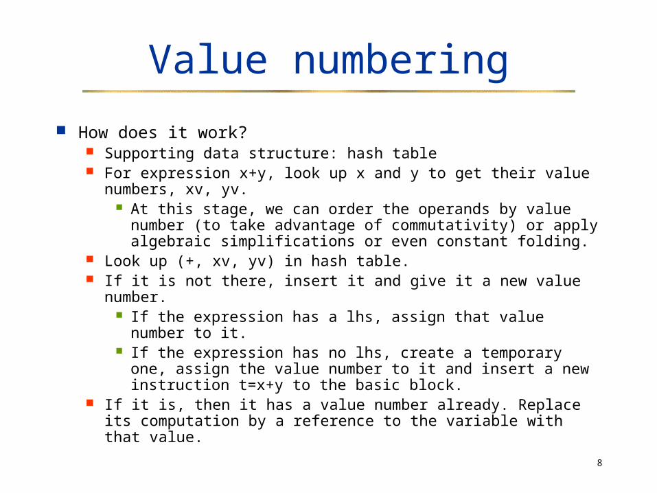
How does it work? Supporting data structure: hash table For expression x+y, look up x and y to get their value
numbers, xv, yv. At this stage, we can order the operands by value
number (to take advantage of commutativity) or apply algebraic simplifications or even constant folding.
Look up (+, xv, yv) in hash table. If it is not there, insert it and give it a new value number.
If the expression has a lhs, assign that value number to it.
If the expression has no lhs, create a temporary one, assign the value number to it and insert a new instruction t=x+y to the basic block.
If it is, then it has a value number already. Replace its computation by a reference to the variable with that value.
9
Value numbering
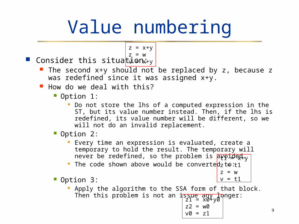
Consider this situation: The second x+y should not be replaced by z, because z
was redefined since it was assigned x+y. How do we deal with this?
Option 1: Do not store the lhs of a computed expression in the ST,
but its value number instead. Then, if the lhs is redefined, its value number will be different, so we will not do an invalid replacement.
Option 2: Every time an expression is evaluated, create a temporary
to hold the result. The temporary will never be redefined, so the problem is avoided.
The code shown above would be converted to:
Option 3: Apply the algorithm to the SSA form of that block. Then
this problem is not an issue any longer:
z = x+yz = wv = x+y
t1 = x+yz = t1z = wv = t1
z1 = x0+y0z2 = w0v0 = z1
10
Local value numbering
Algorithm sketch for local value numbering:
Processing of instruction inst located at BB[n,i]
hashval = Hash(inst.opd, inst.opr1, inst.op2)
If inst matches instruction inst2 in HT[hashval] if inst2 has a lhs, use that in inst
If inst has a lhs remove all instructions in HT that use inst's lhs
If inst has no lhs create new temp insert temp=inst.rhs before inst replace inst with temp
Add i to the equivalence class at hashval.
11
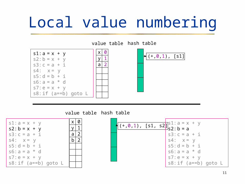
Local value numbering
s1: a =x + ys2: b =x + ys3: c =a + is4: x =ys5: d =b + is6: a =a * ds7: e =x + ys8: if (a==b) goto L
hash table
(+,0,1), [s1]
value table
x 0y 1
hash table
(+,0,1), [s1, s2]
value table
x 0y 1
a 2
a 2b 2
s1: a =x + ys2: b =x + ys3: c =a + is4: x =ys5: d =b + is6: a =a * ds7: e =x + ys8: if (a==b) goto L
s1: a =x + ys2: b =as3: c =a + is4: x =ys5: d =b + is6: a =a * ds7: e =x + ys8: if (a==b) goto L
12
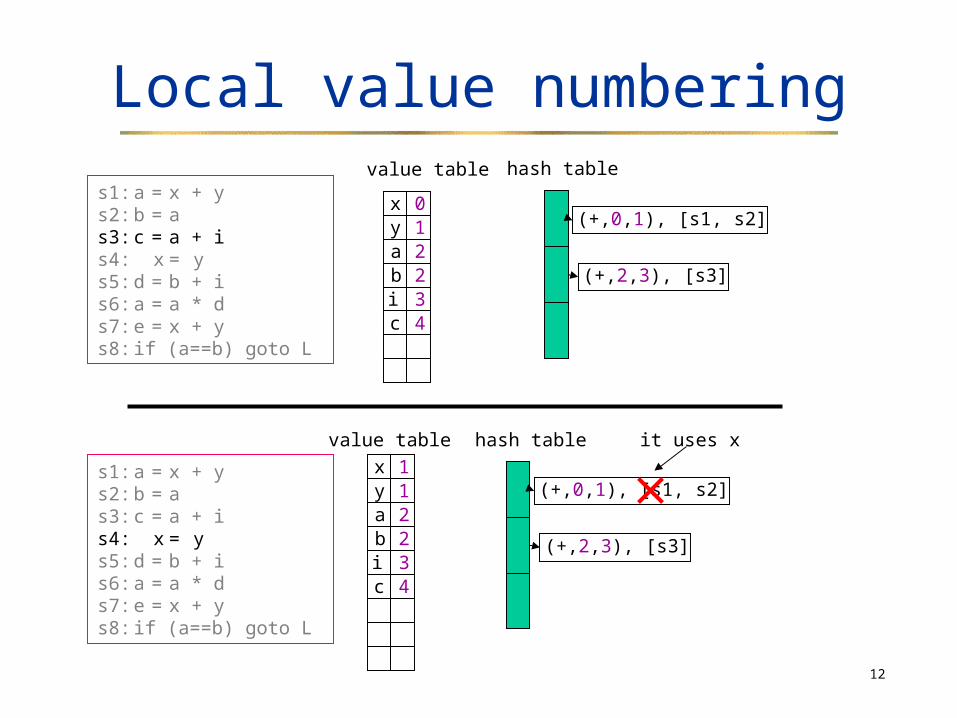
Local value numberinghash table
(+,0,1), [s1, s2]
value table
x 0y 1a 2b 2i 3
(+,2,3), [s3]
c 4
hash table
(+,0,1), [s1, s2]
value table
(+,2,3), [s3]
x 1y 1a 2b 2i 3c 4
s1: a =x + ys2: b =as3: c =a + is4: x =ys5: d =b + is6: a =a * ds7: e =x + ys8: if (a==b) goto L
s1: a =x + ys2: b =as3: c =a + is4: x =ys5: d =b + is6: a =a * ds7: e =x + ys8: if (a==b) goto L
it uses x
13
Local value numberinghash table
(+,0,1), [s2]
value table
(+,2,3), [s3, s5]
x 1y 1a 2b 2i 3c 4
s1: a =x + ys2: b =as3: c =a + is4: x =ys5: d =b + is6: a =a * ds7: e =x + ys8: if (a==b) goto L
s1: a =x + ys2: b =as3: c =a + is4: x =ys5: d =cs6: a =a * ds7: e =x + ys8: if (a==b) goto L
d 4
hash table
(+,0,1), [s2]
value table
(+,2,3), [s3, s5]
x 1y 1a 5b 2i 3c 4
s1: a =x + ys2: b =as3: c =a + is4: x =ys5: d =cs6: a =a * ds7: e =x + ys8: if (a==b) goto L
d 4
(*,2,4), [s6]
14
Local value numberinghash table
(+,0,1), []
value table
(+,2,3), [s5]
x 1y 1a 5b 2i 3c 4
s1: a =x + ys2: b =as3: c =a + is4: x =ys5: d =cs6: a =a * ds7: e =x + ys8: if (a==b) goto L
d 4
(*,2,4), [s6]
(+,1,1), [s7]
e 6
hash table
(+,0,1), []
value table
(+,2,3), [s5]
x 1y 1a 5b 2i 3c 4
s1: a =x + ys2: b =as3: c =a + is4: x =ys5: d =cs6: a =a * ds7: e =x + ys8: if (a==b) goto L
d 4
(*,2,4), [s6]
(+,1,1), [s7]
e 6
(==,2,5), [s8]
t 7
Note how the value numbers forthis expression's operands are sorted, to take advantage ofcommutativity
s1: a =x + ys2: b =as3: c =a + is4: x =ys5: d =cs6: a =a * ds7: e =x + ys8: t =a==bs9: if (t) goto L
15
Local value numbering
value table
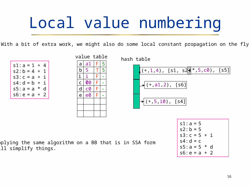
Adding an is_constant entry to the value table, along with the value of the constant, would allow us to incorporate constant folding. We will use SSA numbering for a variable'svalue number and the actual value for a constant's value number.
s1: a =1 + 4s2: b =4 + 1s3: c =a + is4: d =b + is5: a =a * ds6: e =a + 2
s1: a =5s2: b =5s3: c =a + is4: d =cs5: a =a * ds6: e =a + 2
hash table
(+,1,4), [s1, s2]
(+,a1,2), [s6]
(*,5,c0), [s5]
(+,5,i0), [s4]
a a1 F 5b 5 T 5i i
0F -
c c0 F -d c0 F -e e0 F -
16
Local value numberingWith a bit of extra work, we might also do some local constant propagation on the fly.
value table
s1: a =1 + 4s2: b =4 + 1s3: c =a + is4: d =b + is5: a =a * ds6: e =a + 2
s1: a =5s2: b =5s3: c =5 + is4: d =cs5: a =5 * ds6: e =a + 2
hash table
(+,1,4), [s1, s2]
(+,a1,2), [s6]
(*,5,c0), [s5]
(+,5,i0), [s4]
a a1 F 5b 5 T 5i i
0F -
c c0 F -d c0 F -e e0 F -
Applying the same algorithm on a BB that is in SSA formwill simplify things.
17
Superlocal value numbering
Each path on the EBB should be handled separately
However, some blocks are prefixes of more than one EBB. We'd like to avoid recomputing the values in those
blocks Possible solutions :
Use a mechanism similar to those for lexical scope handling
Save the state of the table at the end of each BB
18
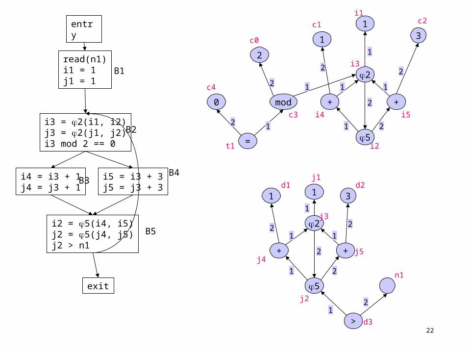
Global value numbering
Main Idea: Variable equivalence Two variables are equivalent at point P iff
they are congruent and their defining assignments dominate P
Two variables are congruent iff their definitions have identical operators and congruent operands.
We need SSA form
19
Global value numbering
Data structure: The Value Graph. Nodes are labeled with
operators function symbols constant values
Nodes are named using SSA-form variables Edges point
from operators or functions to operands
Edges are labeled with numbers that indicate operand position
20
Global value numbering
In the Value Graph: Two nodes are congruent iff
They are the same node, OR Their labels are constants and the constants have the
same value, OR Their labels are the same operator and their operands
are congruent. Algorithm sketch:
Partition nodes into congruent sets Initial partition is optimistic: nodes with the same label are
placed together Note: An alternative would be a pessimistic version,
where initial sets are empty and then fill up in a monotonic way.
Iterate to a fixed point, splitting partitions where operands are not congruent.
21
entry
read(n)i = 1j = 1
i mod 2 == 0
i = i + 1j = j + 1
i = i + 3j = j + 3
j > n
exit
B1
B2
B3 B4
B5
entry
read(n1)i1 = 1j1 = 1
i3 = 2(i1, i2)j3 = 2(j1, j2)i3 mod 2 == 0
i4 = i3 + 1j4 = j3 + 1
i5 = i3 + 3j5 = j3 + 3
i2 = 5(i4, i5)j2 = 5(j4, j5)j2 > n1
exit
B1
B2
B3B4
B5
22
entry
read(n1)i1 = 1j1 = 1
i3 = 2(i1, i2)j3 = 2(j1, j2)i3 mod 2 == 0
i4 = i3 + 1j4 = j3 + 1
i5 = i3 + 3j5 = j3 + 3
i2 = 5(i4, i5)j2 = 5(j4, j5)j2 > n1
exit
B1
B2
B3B4
B5
0
2
1
13
2
+ +
5=
mod
1 1 3
2
+ +
5
>
1
1
1
11
1
1 1
1
1
1
2
2
2 2
2
2 2
2
2
2
c0
c4
c1
i1c2
2
t1
c3
i3
i4 i5
i2
j1d1 d2
j3
j4j5
j2
d3
n1
23
0
2
1
13
2
+ +
5=
mod
1 1 3
2
+ +
5
>
1
1
1
11
1
1 1
1
1
1
2
2
2 2
2
2 2
2
2
2
c0
c4
c1
i1c2
2
t1
c3
i3
i4 i5
i2
j1d1 d2
j3
j4j5
j2
d3
n1
Initially, nodes that have the same labelare placed in the same set.
The initial partition is shown on the left.
Nodes that are in the same set, have thesame color.
i4 and j4 are congruent because theiroperands are congruent.Similarly, i5 and j5 are congruent.However, i4 and i5 are not.The "red" partition needs to be split
Exercise: How would the partitions change if i5 contained a minus?
Answer: <click here>
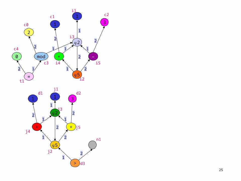
24
0
2
1
13
2
+ –
5=
mod
1 1 3
2
+ +
5
>
1
1
1
11
1
1 1
1
1
1
2
2
2 2
2
2 2
2
2
2
c0
c4
c1
i1c2
2
t1
c3
i3
i4 i5
i2
j1d1 d2
j3
j4j5
j2
d3
n1
The initial partition is shown on the left.
Nodes that are in the same set, have thesame color.
As you can see, i5 and j5 are not congruent this time, since they are labeled differently.
This, in turn, means that i2 and j2 are not congruent, so that set should be split.
As a result of that, i3 and j3 are now not congruent.