1

OUTPUT ANALYSIS FOR SIMULATIONS

2

Introduction Analysis of One System Terminating vs. Steady-State

Simulations Analysis of Terminating

Simulations Obtaining a Specified Precision Analysis of Steady-State

Simulations Method of Batch Means

Outline

3

Introduction

After understanding the under laying process, collecting data, fitting data to a distribution, coding and debugging the simulation program selecting a performance measure to

evaluate the system evaluating your design by runs

But by doing one or two runs, is it enough to evaluate your system? Answer is No. Because components driving your

simulation include randomness, the output of simulation is also random

The output is not independent and identically distributed (i.i.d), we can not use classical statistical methods

4

What Outputs to Watch?

Performance measure - criteria that evaluate how god your system is Average, and worst (longest) time in

system

Average, and worst time in queue(s)

Average hourly production

Standard deviation of hourly production

Proportion of time a machine is up, idle,

or down

Maximum queue length

Average number of parts in system

5

Types of Simulations with Regard to Output Analysis

Transient : A simulation where there is a specific starting and stopping condition that is part of the model. transient performance measures:the performance of system finite horizon

Steady-state: A simulation where there is no specific starting and ending conditions. Here, we are interested in the steady-state behavior of the system. Steady-state performance measures: the

performance for infinite horizon

“The type of analysis depends on the goal of the study.”

6

Analysis for Transient Simulations

Objective: Obtain a point estimate and confidence interval for some parameter

Examples:= E (average time in system for n customers)

= E (machine utilization)

= E (work-in-process)

Reminder: Can not use classical statistical

methods within a simulation run because

observations from one run are not independently

and identically distributed (i.i.d.)

7

Analysis for Transient Simulations

Make n independent replications of the model

Let Yi be the performance measure from the ith replicationYi = average time in system, orYi = work-in-process, or Yi = utilization of a critical facility

Performance measures from different replications, Y1, Y2, ..., Yn, are i.i.d.

But, only one sample is obtained from each replication

Apply classical statistics to Yi’s, not to observations within a run

Select confidence level 1 – (0.90, 0.95, etc.)

8

Analysis for Transient Simulations

Approximate 100(1 – a)% confidence interval for :

estimator of

estimator of Var(Yi)

covers with approximate

probability (1 – a)

is the Half-Width expression

Y nY

n

ii

n

( ) 1

S nY Y n

n

ii

n

2

2

1

1( )

[ ( )]

Y n tS n

nn( )( )

, 1 1 2

( , )( )

,n tS n

nn 1 1 2

9

Consider a single-server (M/M/1) queue. The objective is to calculate a confidence interval for the delay of customers in the queue.

n = 10 replications of a single-server queueYi = average delay in queue from ith replication

Yi’s: 2.02, 0.73, 3.20, 6.23, 1.76, 0.47, 3.89, 5.45, 1.44, 1.23

For 90% confidence interval, = 0.10

= 2.64, = 3.96, t9, 0.95 = 1.833

Approximate 90% confidence interval is

2.64 ± 1.15, or [1.49, 3.79]

Example

Y( )10 S 2 10( )

10

Analysis for Transient Simulations

Interpretation: 100(1 – a)% of the time, the confidence interval formed in this way covers

Wrong Interpretation: “I am 90% confident

that is between 1.49 and 3.79”

(unknown)

11

Issue 1

This confidence-interval method assumes Yi’s are normally distributed. In real life, this is almost never true.

Because of central-limit theorem, as the number of replications (n) grows, the coverage probability approaches 1 – a.

In general, if Yi’s are averages of something, their distribution tends not to be too asymmetric, and the confidence- interval method shown above has reasonably good coverage.

12

The confidence interval may be too wide

In the M/M/1 queue example, the approximate 90% C.I. was:2.64 ± 1.15, or [1.49, 3.79]

The half-width is 1.15 which is 44% of the mean (1.15/2.64)

That means that the C.I. is 2.64 44% which is not very precise.

To decrease the half-width:Increase n until is small enough (this is called Sequential Sampling)

There are two ways of defining the precision in the estimate Y: Absolute precision Relative precision

Issue 2

( , )n

13

Obtaining a Specified Precision

14

Obtaining a Specified Precision

15

Obtaining a Specified Precision

Relative Precision:

16

Analysis for Steady-State Simulations

Objective: Estimate the steady state mean

Basic question: Should you do many short runs or one long run ?????

lim ( )i iE Y

Many short runs

One long run

X1

X2

X3

X4

X5

X1

17

Analysis for Steady-State Simulations

Advantages: Many short runs:

Simple analysis, similar to the analysis for terminating systems

The data from different replications are i.i.d. One long run:

Less initial bias No restarts

Disadvantages Many short runs:

Initial bias is introduced several times One long run:

Sample of size 1 Difficult to get a good estimate of the variance

18

Analysis for Steady-State Simulations

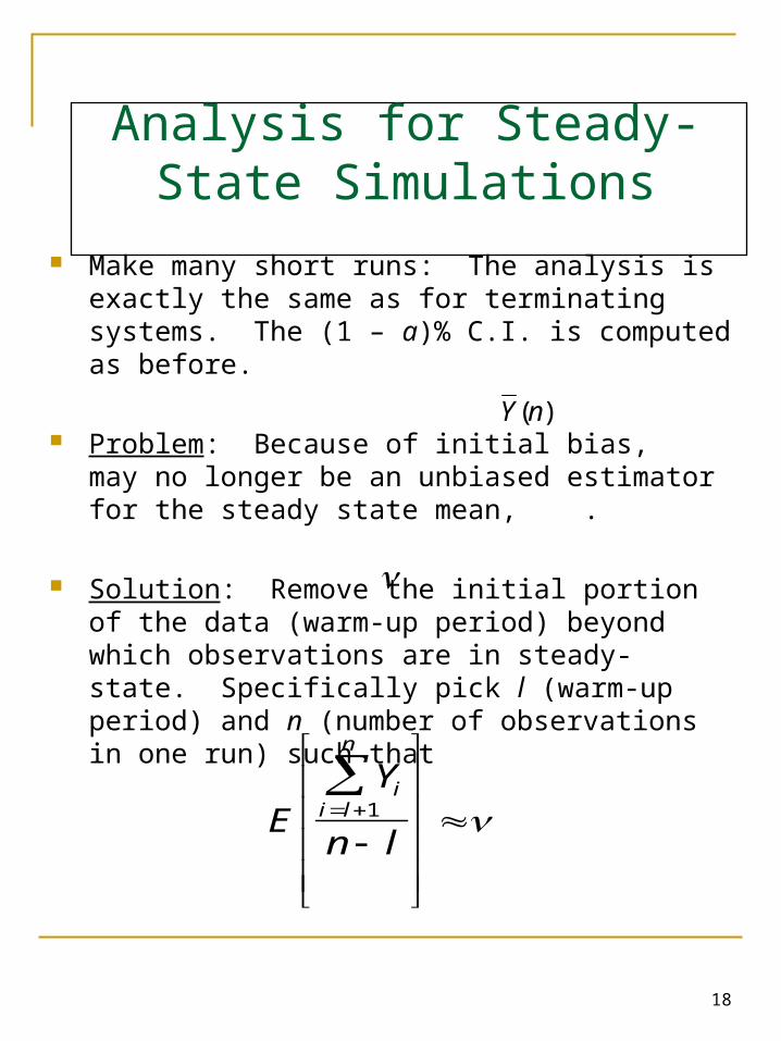
Make many short runs: The analysis is exactly the same as for terminating systems. The (1 – a)% C.I. is computed as before.

Problem: Because of initial bias, may no longer be an unbiased estimator for the steady state mean, .

Solution: Remove the initial portion of the data (warm-up period) beyond which observations are in steady-state. Specifically pick l (warm-up period) and n (number of observations in one run) such that

Y n( )

EY

n l

ii l

n

1

19

Analysis for Steady-State Simulations

Make one Long run: Make just one long replication so that the initial bias is only introduced once. This way, you will not be “throwing out” a lot of data.

Problem: How do you estimate the variance because there is only one run?

Solution: Several methods to estimate the variance: Batch means (only approach to be discussed) Time-series models Spectral analysis Standardized time series

20

Method of Batch Means

Divide a run of length m into n adjacent “batches” of length k where m = nk.

Let be the sample or (batch) mean of the jth batch.

The grand sample mean is computed as

Y j

i

Yi

k k k k k

Y 1 Y 2 Y 3 Y 4 Y 5 m nk

Y

Y

Y

n

Y

m

jj

n

ii

m

1 1

21

Method of Batch Means

The sample variance is computed as

The approximate 100(1 – a )% confidence interval for is

S n

Y Y

nY

jj

n

2

2

1

1( )

( )

Y tS n

nnY 1 1 2,

( )

22

Method of Batch Means

Two important issues:

Issue 1: How do we choose the batch size k? Choose the batch size k large enough

so that the batch means, are

approximately uncorrelated.

Otherwise, the variance, , will be

biased low and the confidence interval

will be too small which means that it

will cover the mean with a probability

lower than the desired probability of

(1 – a ).

Y j ' s

S nY2 ( )

23

Method of Batch Means

Issue 2: How many batches n? Due to autocorrelation, splitting the run into a

larger number of smaller batches, degrades the

quality of each individual batch. Therefore, 20 to

30 batches are sufficient.