1 | Page COMPRESSION ARTIFACT REDUCTION IN HEVC USING ADAPTIVE BILATERAL FILTER by ROHITH REDDY ETIKALA Presented to the Faculty of the Graduate School of The University of Texas at Arlington in Partial Fulfillment of the Requirements for the Degree of MASTER OF SCIENCE IN ELECTRICAL ENGINEERING THE UNIVERSITY OF TEXAS AT ARLINGTON April 2016
Transcript
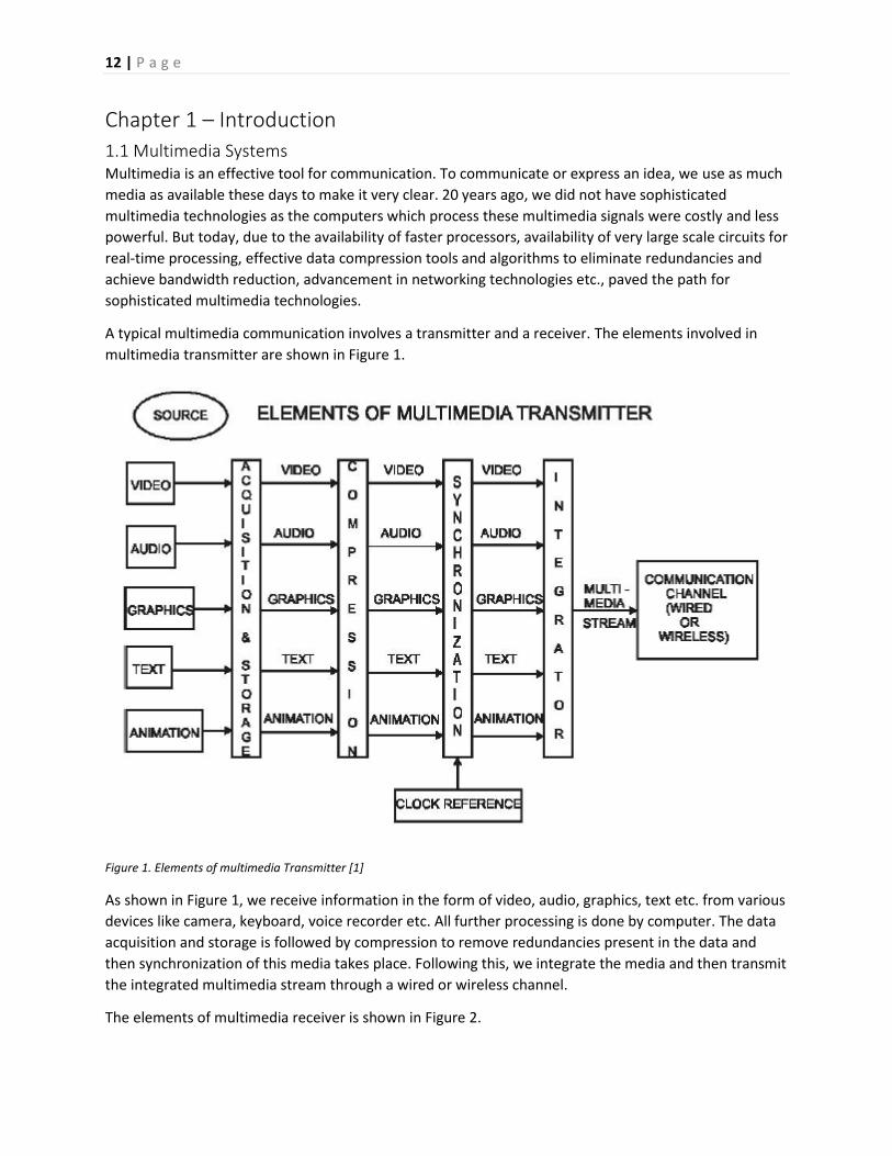
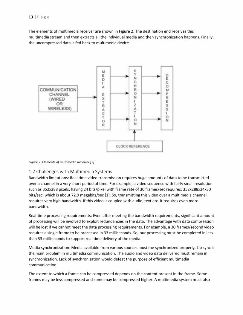
1 | P a g e
COMPRESSION ARTIFACT REDUCTION IN HEVC USING ADAPTIVE BILATERAL FILTER
by
ROHITH REDDY ETIKALA
Presented to the Faculty of the Graduate School of
The University of Texas at Arlington in Partial Fulfillment
List of Acronyms: ......................................................................................................................................... 10
Biographical Information ............................................................................................................................ 83
Figure 44. Example of the ringing effect, where it is most evident around the bright table-edge and the
boundary of the arm [18] ............................................................................................................................ 45
Figure 45. Example of the ringing effect in a sequence coded at a relatively high bit-rate. Most
prominent along the edge formed by the upper-arm in the scene [16] .................................................... 45
Figure 46. Common artifacts due to block based coding. .......................................................................... 46
Karhunen-Love Transforms (KLT) [41], Discrete Wavelet Transforms (DWT) [41] etc.
The quantizer then generates a limited number of symbols that can be used to represent the
transformed data. And, finally coder assigns a code word to each symbol of the quantizer. The code
word can be fixed or variable depending on whether a fixed length or variable length coding technique is
used.
The elements of image de-compression technique are shown in Figure 6. These perform the exact
inverse operations of elements in the image encoding system.
17 | P a g e
Figure 6. Elements of image decoding system [1]
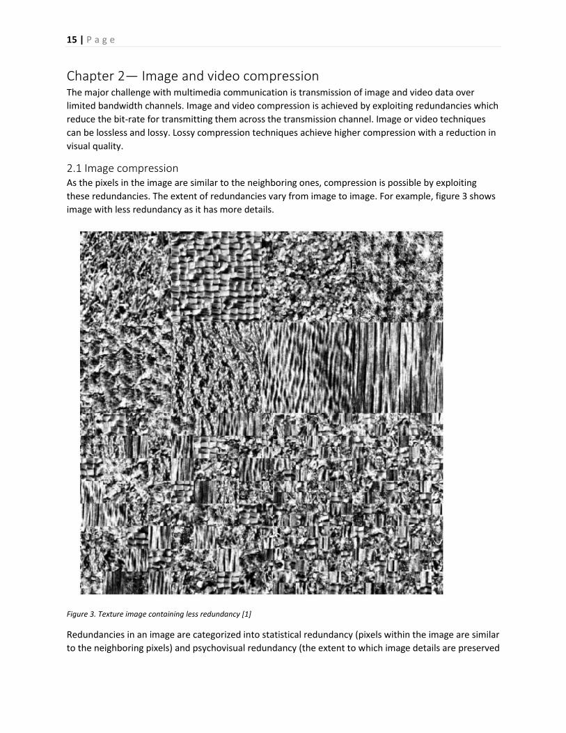
2.2 Image coding standards With the rapid developments of imaging technology, image compression and coding tools and
techniques, it is necessary to develop coding standards so that there is compatibility and interoperability
between the image communication and storage products manufactured by different vendors in the
multimedia market. Without the availability of such standards, encoders and decoders cannot
communicate with one another and hence the service providers will have to support a variety of formats
to meet the needs of the customers and the customers will have to install a number of decoders to
handle a large number of data formats. Towards the objective of setting up coding standards to address
this issue, the international standardization agencies, such as International Standards Organization (ISO),
International Telecommunication Union (ITU), International Electro-technical Commission (IEC) etc. have
formed expert groups and solicited proposals from industries, universities and research laboratories.
These standards use the coding and compression techniques (both lossless and lossy).
The first standard developed for compressing and coding monochrome and color images of any size and
sampling rate was developed by Joint Photographic Experts Group (JPEG) and is known as JPEG. Later
JPEG-2000 has been developed for still images.
The block diagram of JPEG encoder is shown in figure 7.
Figure 7. JPEG Encoder [1]
A more detailed JPEG encoder is shown in figure 8, in which RGB image is converted to YUV image and
then chrominance may be down sampled as human eyes are more sensitive to luminance component
than chrominance.
18 | P a g e
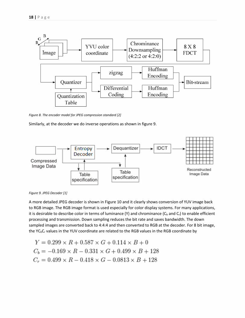
Figure 8. The encoder model for JPEG compression standard [2]
Similarly, at the decoder we do inverse operations as shown in figure 9.
Figure 9. JPEG Decoder [1]
A more detailed JPEG decoder is shown in Figure 10 and it clearly shows conversion of YUV image back
to RGB image. The RGB image format is used especially for color display systems. For many applications,
it is desirable to describe color in terms of luminance (Y) and chrominance (Cb and Cr) to enable efficient
processing and transmission. Down sampling reduces the bit rate and saves bandwidth. The down
sampled images are converted back to 4:4:4 and then converted to RGB at the decoder. For 8 bit image,
the YCbCr values in the YUV coordinate are related to the RGB values in the RGB coordinate by
19 | P a g e
Figure 10. The decoder model for JPEG compression standard [2]
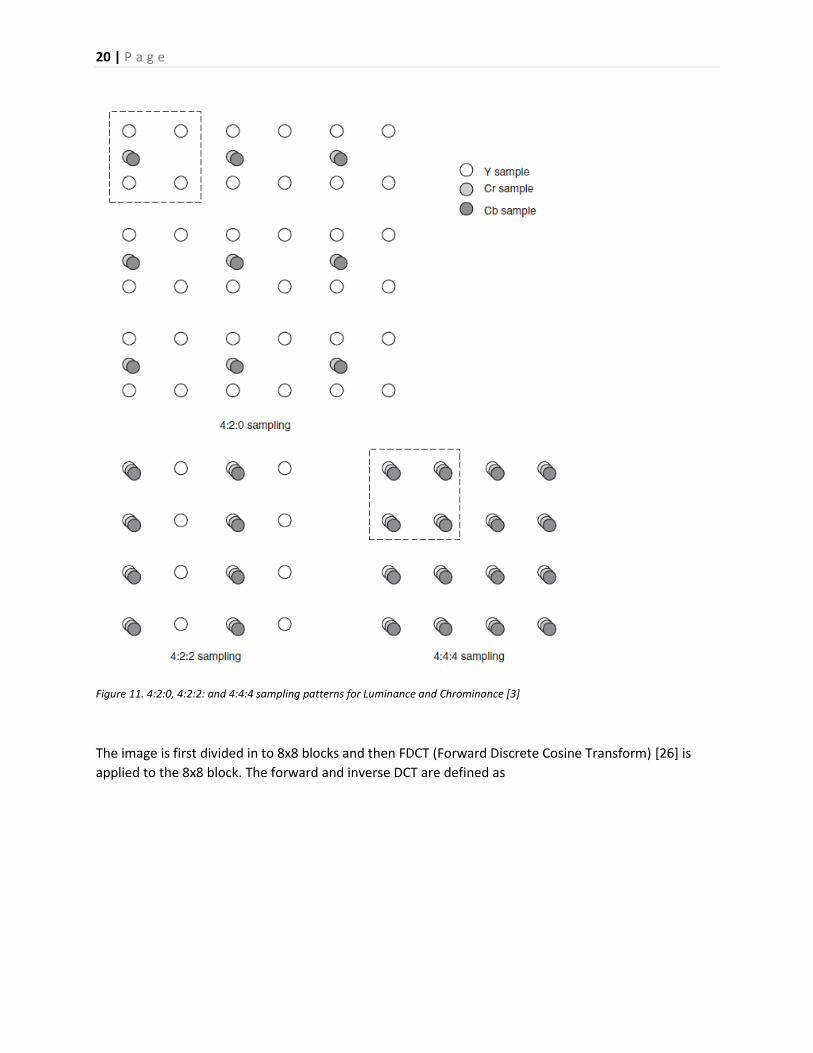
The various sampling patterns (4:2:0, 4:2:2 and 4:4:4) for Luminance and Chrominance supported by
JPEG are shown in Figure 11.
20 | P a g e
Figure 11. 4:2:0, 4:2:2: and 4:4:4 sampling patterns for Luminance and Chrominance [3]
The image is first divided in to 8x8 blocks and then FDCT (Forward Discrete Cosine Transform) [26] is
applied to the 8x8 block. The forward and inverse DCT are defined as
21 | P a g e
The f(x,y) is the value of each pixel in the selected 8×8 block, and the F(u,v) is the DCT coefficient after
transformation. The transformation of the 8×8 block is also a 8×8 block composed of F(u,v). The DCT is a
lossless procedure and the data can be recovered by Inverse DCT. The 8x8 DCT matrix is quantized by
dividing each coefficient by its corresponding quantization value from the default quantization table.
The JPEG committee came up with a 8x8 quantization matrix that works well with performance close to
optimal condition. The quantization matrix for chrominance and luminance are
22 | P a g e
The quantized coefficients (which contain one DC and 63 AC coefficients) are zig-zag scanned as shown
in the Figure 12. Then the coefficients are encoded using Huffman encoding.
Figure 12. Zig-zag scanning order in JPEG [3]
The similar inverse process is followed at the JPEG decoder as shown in figure 10.
JPEG encoding is very popular, but images compressed using JPEG at a very low bit rate show severe
blocking artifacts as we use block based DCT. So, an advanced imaging standard known as JPEG-2000
[38] was developed. JPEG-2000 is based on EBCOT (Embedded Block Coding with Optimized Truncation)
wavelet coding technique.
2.3 Video compression Spatial and temporal sampling of a video is shown in figure 13. Video compression aims at exploiting
redundancies in spatial and temporal domains. Temporal redundancy is exploited by predicting the
current frame using the information from the past frames.
23 | P a g e
Figure 13. Spatial and temporal sampling of a video sequence [3]
The block diagram of a hybrid video encoder is shown in figure 14. The hybrid video decoder is shown in
figure 15. These codecs (encoder and decoder) are popularly called as hybrid codecs as they use
predictive and transform domain techniques. Most of the modern video codecs resemble hybrid video
codec with a slight modification.
The predictive techniques temporally current frame from previously stored frames and it assumes that
video sequences exhibit similarity between consecutive frames. The predicted frame is subtracted from
the current frame and the difference image is obtained. The spatial redundancy in the difference image
is exploited by applying image transforms such as DCT and Integer-DCT and the coefficients are
quantized and entropy coded. The encoded information is sent to the receiver.
The encoder has a built in decoder to reconstruct the difference image. The difference image is added to
the predicted image to generate the buffer. The motion estimation block in the encoder determines the
displacement between current frame and previously stored frames. The displacements computed are
applied on the stored frames to obtain the predicted frame.
24 | P a g e
Figure 14. Hybrid video encoder [1]
Figure 15. Hybrid video decoder [1]
A video sequence itself is considered to have a group of pictures as shown in figure 16.
25 | P a g e
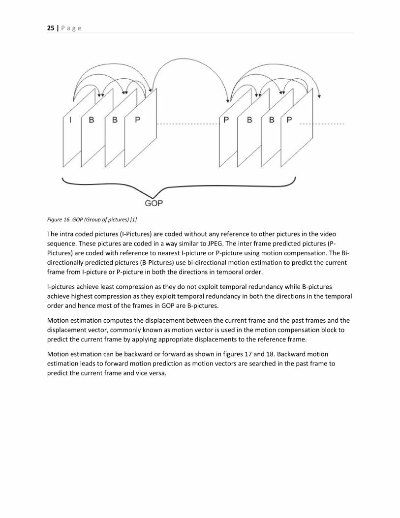
Figure 16. GOP (Group of pictures) [1]
The intra coded pictures (I-Pictures) are coded without any reference to other pictures in the video
sequence. These pictures are coded in a way similar to JPEG. The inter frame predicted pictures (P-
Pictures) are coded with reference to nearest I-picture or P-picture using motion compensation. The Bi-
directionally predicted pictures (B-Pictures) use bi-directional motion estimation to predict the current
frame from I-picture or P-picture in both the directions in temporal order.
I-pictures achieve least compression as they do not exploit temporal redundancy while B-pictures
achieve highest compression as they exploit temporal redundancy in both the directions in the temporal
order and hence most of the frames in GOP are B-pictures.
Motion estimation computes the displacement between the current frame and the past frames and the
displacement vector, commonly known as motion vector is used in the motion compensation block to
predict the current frame by applying appropriate displacements to the reference frame.
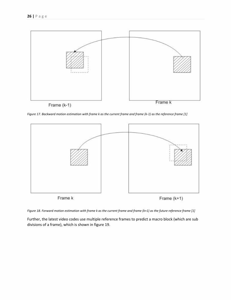
Motion estimation can be backward or forward as shown in figures 17 and 18. Backward motion
estimation leads to forward motion prediction as motion vectors are searched in the past frame to
predict the current frame and vice versa.
26 | P a g e
Figure 17. Backward motion estimation with frame k as the current frame and frame (k-1) as the reference frame [1]
Figure 18. Forward motion estimation with frame k as the current frame and frame (k+1) as the future reference frame [1]
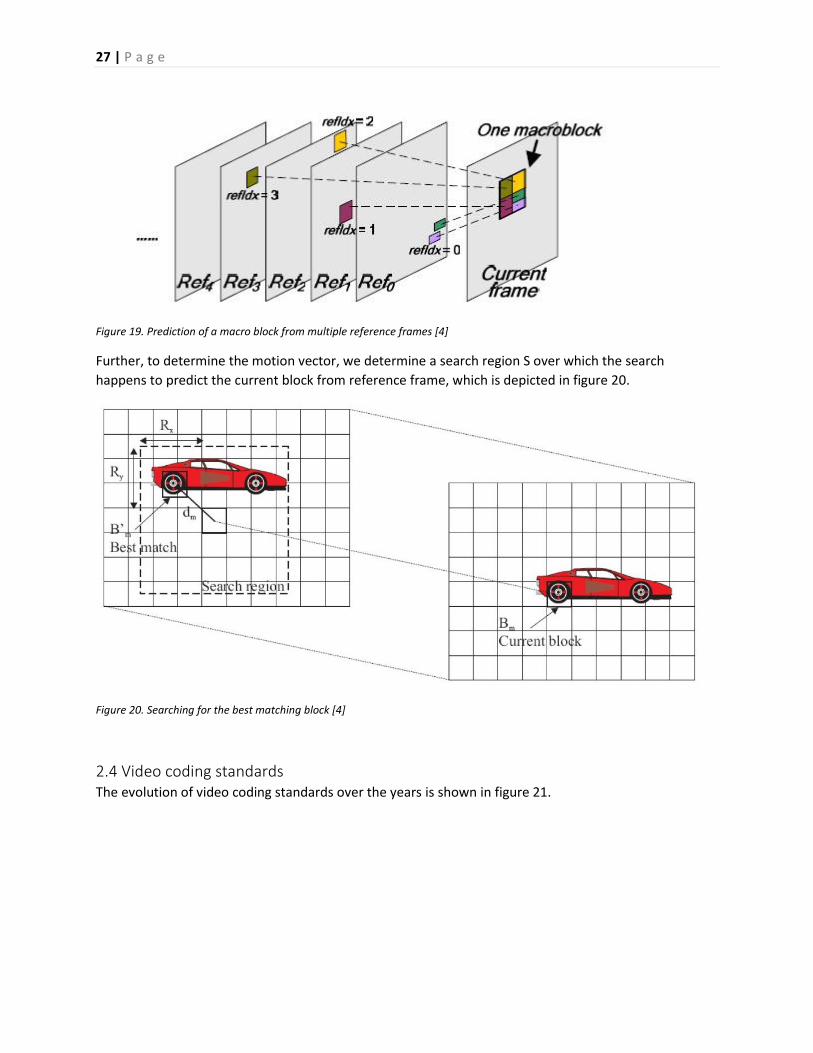
Further, the latest video codes use multiple reference frames to predict a macro block (which are sub
divisions of a frame), which is shown in figure 19.
27 | P a g e
Figure 19. Prediction of a macro block from multiple reference frames [4]
Further, to determine the motion vector, we determine a search region S over which the search
happens to predict the current block from reference frame, which is depicted in figure 20.
Figure 20. Searching for the best matching block [4]
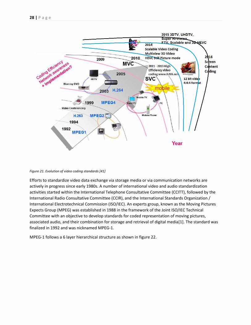
2.4 Video coding standards The evolution of video coding standards over the years is shown in figure 21.
28 | P a g e
Figure 21. Evolution of video coding standards [41]
Efforts to standardize video data exchange via storage media or via communication networks are
actively in progress since early 1980s. A number of international video and audio standardization
activities started within the International Telephone Consultative Committee (CCITT), followed by the
International Radio Consultative Committee (CCIR), and the International Standards Organization /
International Electrotechnical Commission (ISO/IEC). An experts group, known as the Moving Pictures
Expects Group (MPEG) was established in 1988 in the framework of the Joint ISO/IEC Technical
Committee with an objective to develop standards for coded representation of moving pictures,
associated audio, and their combination for storage and retrieval of digital media[1]. The standard was
finalized in 1992 and was nicknamed MPEG-1.
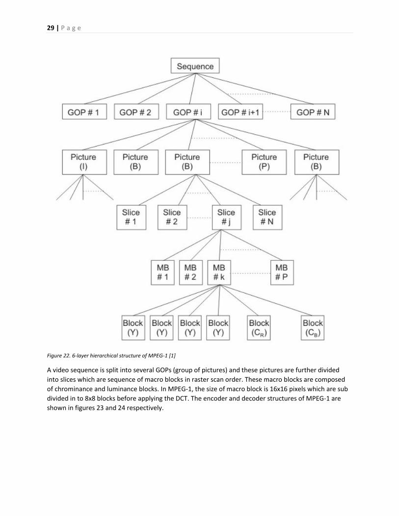
MPEG-1 follows a 6 layer hierarchical structure as shown in figure 22.
29 | P a g e
Figure 22. 6-layer hierarchical structure of MPEG-1 [1]
A video sequence is split into several GOPs (group of pictures) and these pictures are further divided
into slices which are sequence of macro blocks in raster scan order. These macro blocks are composed
of chrominance and luminance blocks. In MPEG-1, the size of macro block is 16x16 pixels which are sub
divided in to 8x8 blocks before applying the DCT. The encoder and decoder structures of MPEG-1 are
shown in figures 23 and 24 respectively.
30 | P a g e
DCT Q
Q-1
IDCT
Motion
Compensation
Motion
Estimation
Entropy
Coding
Input
Video
Frame
Memory
Compressed
Video
Figure 23. Encoder structure of MPEG-1 [4]
Figure 24. Simplified decoder structure of MPEG-1 [6]
MPEG-1 was the first ISO/IEC standard that was primarily targeted for a bit-rate up to 1.5 megabits/sec
for digital storage of video on CDs. The standard was adopted in 1992. As newer application areas like
video broadcasting and HDTV emerged, there was a need to develop new standards [1].
MPEG continued its standardization efforts and the next standard, MPEG-2 [42] was given the charter to
provide video quality not lower than NTSC/PAL. Video coding for broadcast and storing video on digital
video disks (DVD) with an order of 2-15 megabits/sec allocated to audio and video coding were
addressed by MPEG-2. MPEG-2 addresses the emerging applications like digital cable television
distribution, high definitions televisions (HDTV), satellite digital video broadcasts, networked multimedia
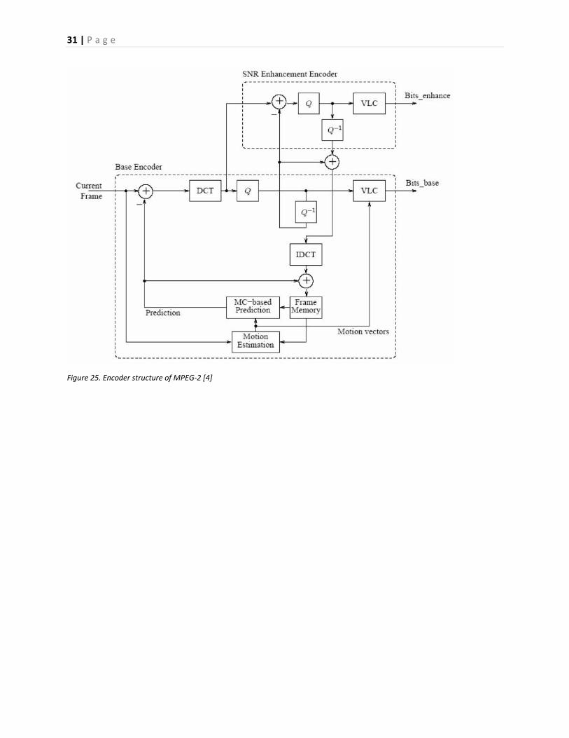
through ATM etc. The encoder and decoder structure of MPEG-2 are shown in figures 25 and 26
respectively.
31 | P a g e
Figure 25. Encoder structure of MPEG-2 [4]
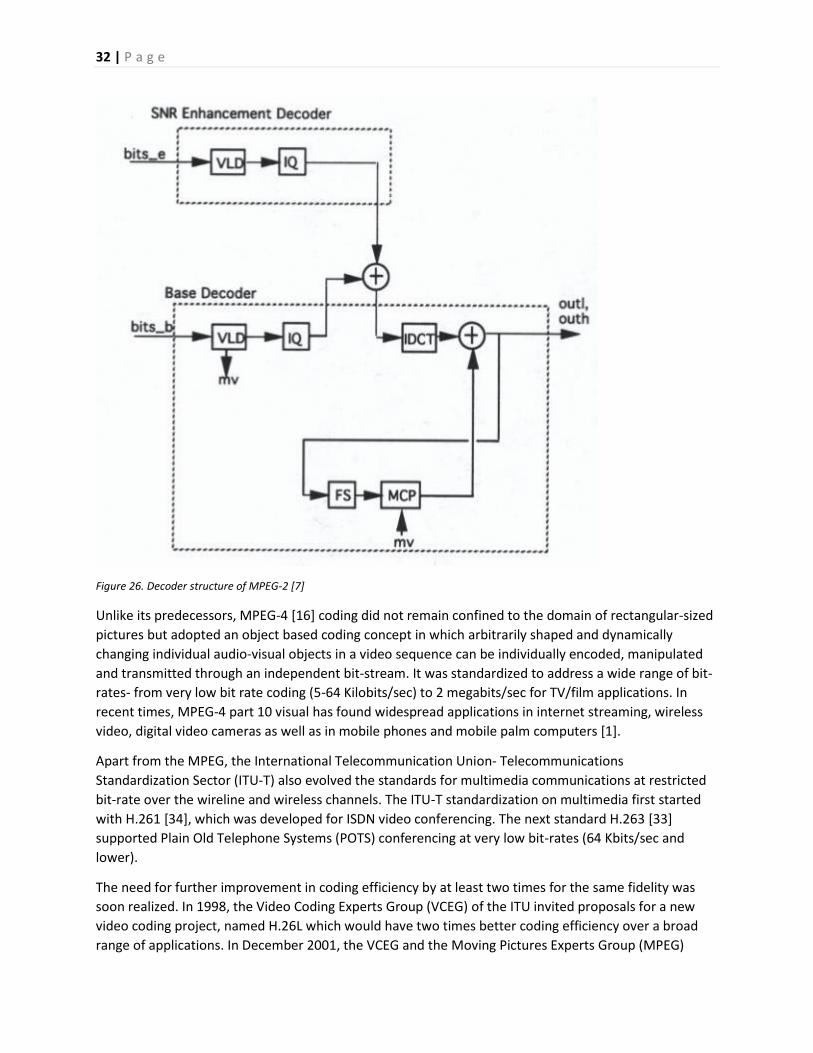
32 | P a g e
Figure 26. Decoder structure of MPEG-2 [7]
Unlike its predecessors, MPEG-4 [16] coding did not remain confined to the domain of rectangular-sized
pictures but adopted an object based coding concept in which arbitrarily shaped and dynamically
changing individual audio-visual objects in a video sequence can be individually encoded, manipulated
and transmitted through an independent bit-stream. It was standardized to address a wide range of bit-
rates- from very low bit rate coding (5-64 Kilobits/sec) to 2 megabits/sec for TV/film applications. In
recent times, MPEG-4 part 10 visual has found widespread applications in internet streaming, wireless
video, digital video cameras as well as in mobile phones and mobile palm computers [1].
Apart from the MPEG, the International Telecommunication Union- Telecommunications
Standardization Sector (ITU-T) also evolved the standards for multimedia communications at restricted
bit-rate over the wireline and wireless channels. The ITU-T standardization on multimedia first started
with H.261 [34], which was developed for ISDN video conferencing. The next standard H.263 [33]
supported Plain Old Telephone Systems (POTS) conferencing at very low bit-rates (64 Kbits/sec and
lower).
The need for further improvement in coding efficiency by at least two times for the same fidelity was
soon realized. In 1998, the Video Coding Experts Group (VCEG) of the ITU invited proposals for a new
video coding project, named H.26L which would have two times better coding efficiency over a broad
range of applications. In December 2001, the VCEG and the Moving Pictures Experts Group (MPEG)
33 | P a g e
formed a Joint Video Team (JVT). Their combined efforts resulted in the new coding standard H.264. This
also forms the Part-10 (Advanced Video Coding) of MPEG-4 and is therefore referred to as H.264 / AVC
standard.
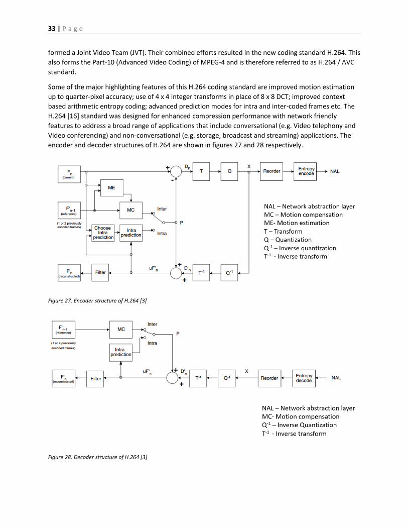
Some of the major highlighting features of this H.264 coding standard are improved motion estimation
up to quarter-pixel accuracy; use of 4 x 4 integer transforms in place of 8 x 8 DCT; improved context
based arithmetic entropy coding; advanced prediction modes for intra and inter-coded frames etc. The
H.264 [16] standard was designed for enhanced compression performance with network friendly
features to address a broad range of applications that include conversational (e.g. Video telephony and
Video conferencing) and non-conversational (e.g. storage, broadcast and streaming) applications. The
encoder and decoder structures of H.264 are shown in figures 27 and 28 respectively.
Figure 27. Encoder structure of H.264 [3]
Figure 28. Decoder structure of H.264 [3]
34 | P a g e
High Efficiency Video Coding Standard (HEVC) was developed after H.264 to provide support for 4K and
8K videos and to support parallel processing architectures. This is discussed in detail in chapter 3.
35 | P a g e
Chapter 3 – High Efficiency Video Coding (HEVC) Standard The High Efficiency Video Coding (HEVC) [8] is the latest video standard developed by Joint Collaborative
Team on Video Coding (JCT-VC), a group of video coding experts from ITU-T Video Coding Experts Group
and SO/IEC Moving Picture Experts Group (MPEG).
As the demand for HD video (4K and 8K) increased, there is a need for stronger coding efficiency than
H.264/AVC. Also, there is increased use of parallel processors. So, HEVC [8] has been introduced to
support increased video resolution and parallel processing. HEVC obtains about 50% reduction in bit rate
when compared to its predecessor H.264/AVC at the same visual quality.
3.1 HEVC encoder and decoder: The block diagrams for HEVC encoder and decoder are shown in figures 29 and 30 respectively. The
input video is split into multiple Coding Tree Units (CTUs) which are predicted using intra/inter
prediction. The residual image is transformed, scaled, quantized and then entropy coded.
Figure 29. Block Diagram of HEVC Encoder [8].
Similarly, the decoder performs entropy decoding followed by rescaling, inverse transform and then
prediction unit is added to reconstruct the video. This process is clearly depicted in Figure 30.
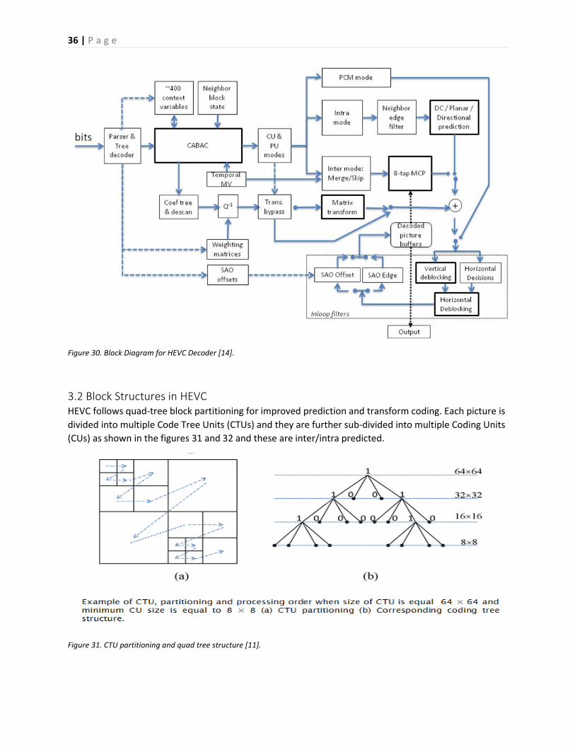
36 | P a g e
Figure 30. Block Diagram for HEVC Decoder [14].
3.2 Block Structures in HEVC HEVC follows quad-tree block partitioning for improved prediction and transform coding. Each picture is
divided into multiple Code Tree Units (CTUs) and they are further sub-divided into multiple Coding Units
(CUs) as shown in the figures 31 and 32 and these are inter/intra predicted.
Figure 31. CTU partitioning and quad tree structure [11].
37 | P a g e
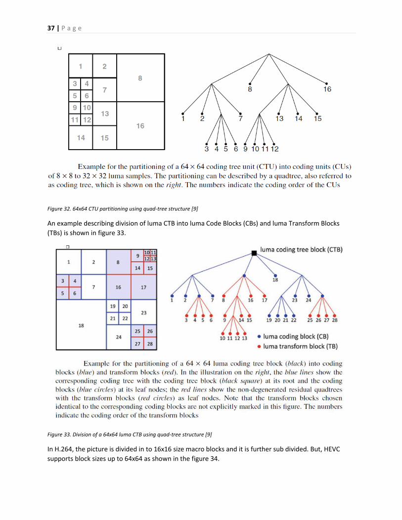
Figure 32. 64x64 CTU partitioning using quad-tree structure [9]
An example describing division of luma CTB into luma Code Blocks (CBs) and luma Transform Blocks
(TBs) is shown in figure 33.
Figure 33. Division of a 64x64 luma CTB using quad-tree structure [9]
In H.264, the picture is divided in to 16x16 size macro blocks and it is further sub divided. But, HEVC
supports block sizes up to 64x64 as shown in the figure 34.
38 | P a g e
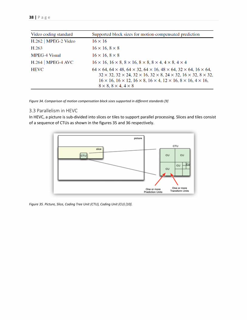
Figure 34. Comparison of motion compensation block sizes supported in different standards [9]
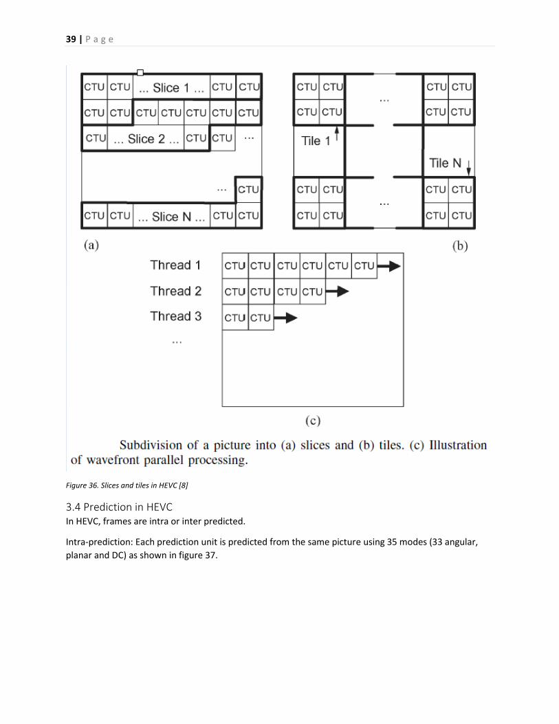
3.3 Parallelism in HEVC In HEVC, a picture is sub-divided into slices or tiles to support parallel processing. Slices and tiles consist
of a sequence of CTUs as shown in the figures 35 and 36 respectively.
Figure 35. Picture, Slice, Coding Tree Unit (CTU), Coding Unit (CU) [10].
39 | P a g e
Figure 36. Slices and tiles in HEVC [8]
3.4 Prediction in HEVC In HEVC, frames are intra or inter predicted.
Intra-prediction: Each prediction unit is predicted from the same picture using 35 modes (33 angular,
planar and DC) as shown in figure 37.
40 | P a g e
Figure 37. Modes and directional orientations for intra prediction in HEVC [8]
Inter-prediction: Each prediction unit is predicted from neighboring picture data using motion
compensated prediction [12] [13] as shown in figure 38.
Figure 38. Illustration of Motion Estimation Process [12]
Further, HEVC uses 7-tap or 8-tap filters for fractional sample interpolation (up to quarter-sample
precision) whereas H.264 uses 6-tap filter for half-sample precision and linear interpolation for quarter-
sample precision. Figure 39 shows integer and fractional sample positions for luma interpolation.
41 | P a g e
Figure 39. Integer and fractional sample positions for luma interpolation [8]
Further, filter coefficients for luma and chroma fractional sample interpolation are shown in figure 40.
Figure 40. Filter coefficients for luma and chroma fractional sample interpolation [8]
3.5 Transform and Quantization Residual CU is transformed by using block transforms such as integer DCT of sizes 32x32, 16x16, 8x8 and
4x4 and then the transformed data is quantized [10] in HEVC.
42 | P a g e
3.6 Entropy Coding Context Adaptive Binary Arithmetic Coding (CABAC) is used to encode quantized transform coefficients
and motion vector data [10] in HEVC.
3.7 In-loop Filters HEVC employs in-loop filters such as deblocking [15] and Sample Adaptive Offset (SAO) [9] as shown in
figure 29, while H.264 employs only deblocking filter. Deblocking filter removes block discontinues due
to transform or prediction at block boundaries. SAO filter reduces ringing artifacts.
43 | P a g e
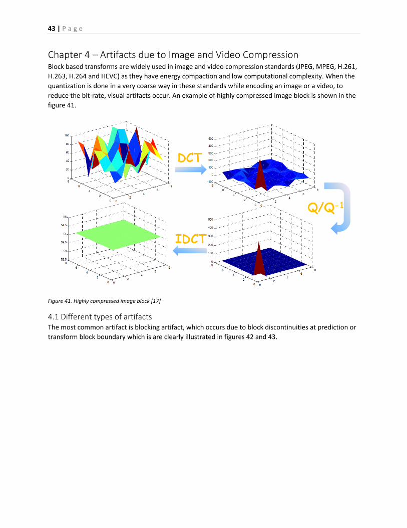
Chapter 4 – Artifacts due to Image and Video Compression Block based transforms are widely used in image and video compression standards (JPEG, MPEG, H.261,
H.263, H.264 and HEVC) as they have energy compaction and low computational complexity. When the
quantization is done in a very coarse way in these standards while encoding an image or a video, to
reduce the bit-rate, visual artifacts occur. An example of highly compressed image block is shown in the
figure 41.
Figure 41. Highly compressed image block [17]
4.1 Different types of artifacts The most common artifact is blocking artifact, which occurs due to block discontinuities at prediction or
transform block boundary which is are clearly illustrated in figures 42 and 43.
44 | P a g e
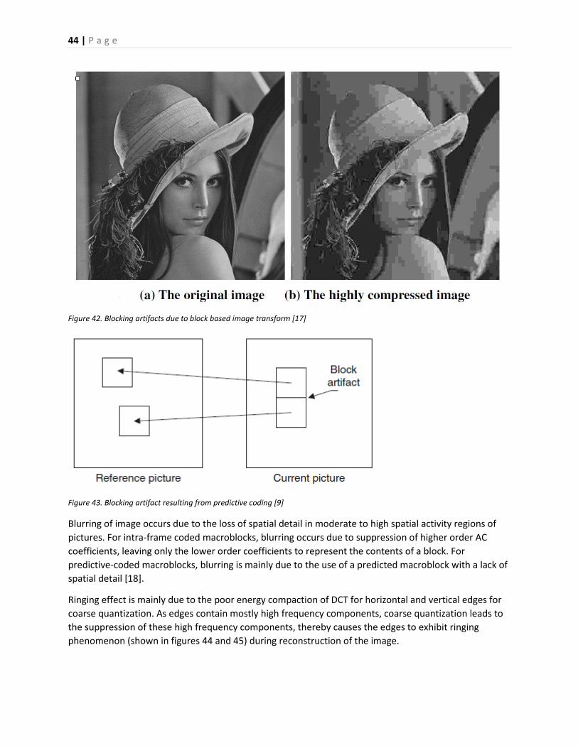
Figure 42. Blocking artifacts due to block based image transform [17]
Figure 43. Blocking artifact resulting from predictive coding [9]
Blurring of image occurs due to the loss of spatial detail in moderate to high spatial activity regions of
pictures. For intra-frame coded macroblocks, blurring occurs due to suppression of higher order AC
coefficients, leaving only the lower order coefficients to represent the contents of a block. For
predictive-coded macroblocks, blurring is mainly due to the use of a predicted macroblock with a lack of
spatial detail [18].
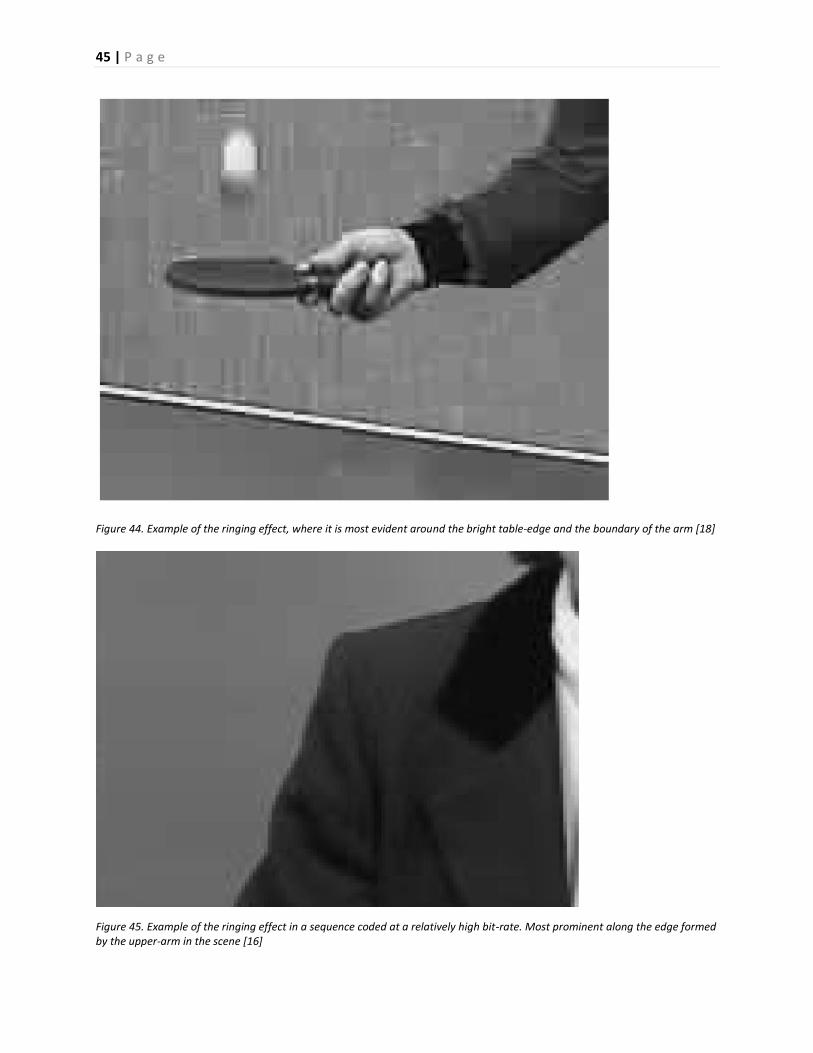
Ringing effect is mainly due to the poor energy compaction of DCT for horizontal and vertical edges for
coarse quantization. As edges contain mostly high frequency components, coarse quantization leads to
the suppression of these high frequency components, thereby causes the edges to exhibit ringing
phenomenon (shown in figures 44 and 45) during reconstruction of the image.
45 | P a g e
Figure 44. Example of the ringing effect, where it is most evident around the bright table-edge and the boundary of the arm [18]
Figure 45. Example of the ringing effect in a sequence coded at a relatively high bit-rate. Most prominent along the edge formed by the upper-arm in the scene [16]
46 | P a g e
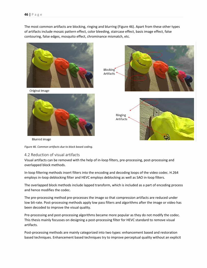
The most common artifacts are blocking, ringing and blurring (Figure 46). Apart from these other types
of artifacts include mosaic pattern effect, color bleeding, staircase effect, basis image effect, false
contouring, false edges, mosquito effect, chrominance mismatch, etc.
Figure 46. Common artifacts due to block based coding.
4.2 Reduction of visual artifacts Visual artifacts can be removed with the help of in-loop filters, pre-processing, post-processing and
overlapped block methods.
In-loop filtering methods insert filters into the encoding and decoding loops of the video codec. H.264
employs in-loop deblocking filter and HEVC employs deblocking as well as SAO in-loop filters.
The overlapped block methods include lapped transform, which is included as a part of encoding process
and hence modifies the codec.
The pre-processing method pre-processes the image so that compression artifacts are reduced under
low bit-rate. Post-processing methods apply low pass filters and algorithms after the image or video has
been decoded to improve the visual quality.
Pre-processing and post-processing algorithms became more popular as they do not modify the codec.
This thesis mainly focusses on designing a post-processing filter for HEVC standard to remove visual
artifacts.
Post-processing methods are mainly categorized into two types: enhancement based and restoration
based techniques. Enhancement based techniques try to improve perceptual quality without an explicit
47 | P a g e
optimization process while restoration techniques recover original image based on some optimization
criteria. This thesis mainly focusses on an enhancement technique using bilateral filter.
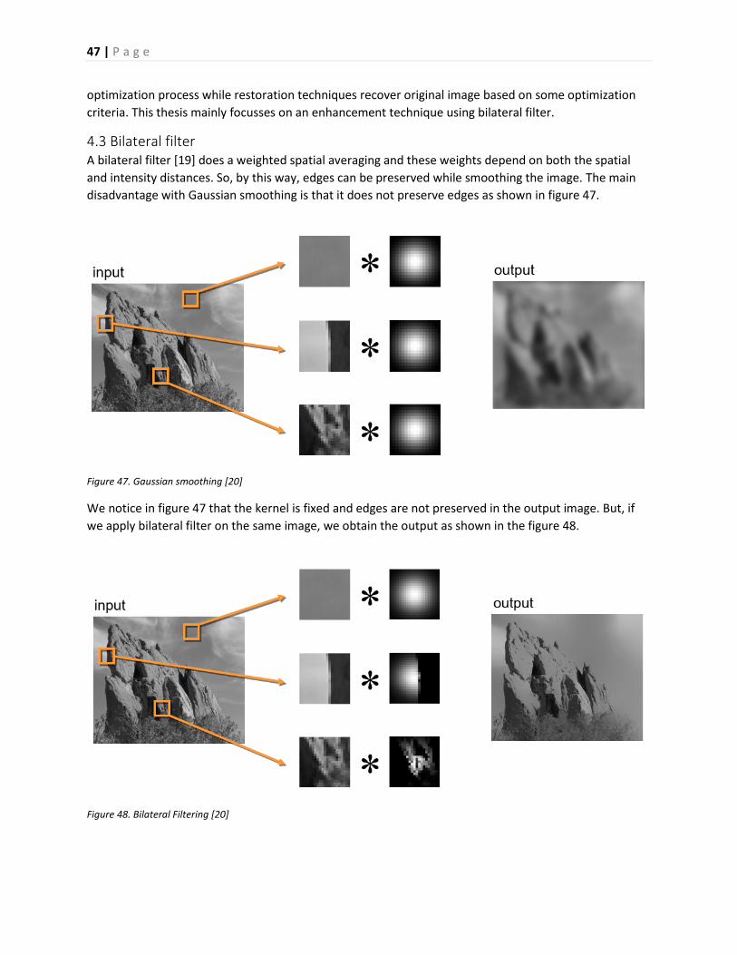
4.3 Bilateral filter A bilateral filter [19] does a weighted spatial averaging and these weights depend on both the spatial
and intensity distances. So, by this way, edges can be preserved while smoothing the image. The main
disadvantage with Gaussian smoothing is that it does not preserve edges as shown in figure 47.
Figure 47. Gaussian smoothing [20]
We notice in figure 47 that the kernel is fixed and edges are not preserved in the output image. But, if
we apply bilateral filter on the same image, we obtain the output as shown in the figure 48.
Figure 48. Bilateral Filtering [20]
48 | P a g e
We notice in figure 48 that, the kernel size depends on the image content and edges are preserved. A
Gaussian filter smoothens edges as it does averaging of pixels across the edges while bilateral filter does
not do averaging of pixels across its edges.
Gaussian blurred image is obtained by applying the 2D Gaussian function at each pixel in the image.
The 2D-Gaussian Function is,
• σ is the standard deviation.
As the size of the kernel or σ increases, the image is strongly smoothened and it is shown in figure 50.
Figure 49. Input image
Figure 50. Limited and strong smoothing [20]
Hence for the Gaussian filter, only spatial distance matters and no special case is considered for edges.
Whereas bilateral filter has an additional edge term as shown in figure 51.
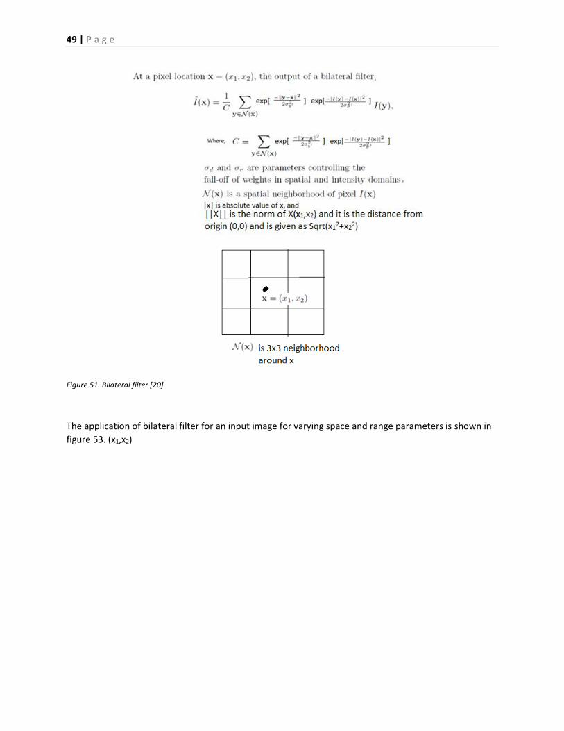
49 | P a g e
Figure 51. Bilateral filter [20]
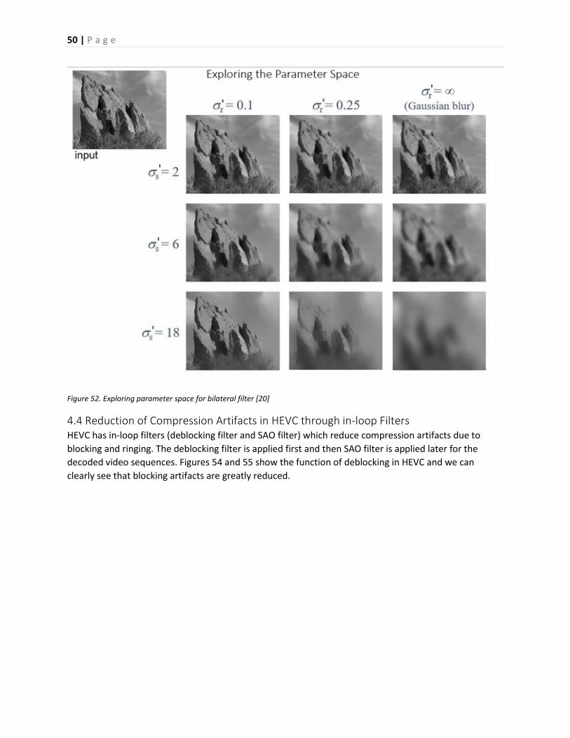
The application of bilateral filter for an input image for varying space and range parameters is shown in
figure 53. (x1,x2)
50 | P a g e
Figure 52. Exploring parameter space for bilateral filter [20]
4.4 Reduction of Compression Artifacts in HEVC through in-loop Filters HEVC has in-loop filters (deblocking filter and SAO filter) which reduce compression artifacts due to
blocking and ringing. The deblocking filter is applied first and then SAO filter is applied later for the
decoded video sequences. Figures 54 and 55 show the function of deblocking in HEVC and we can
clearly see that blocking artifacts are greatly reduced.
51 | P a g e
Figure 53. Performance of Deblocking filter in HEVC for Basketball Drive Sequence [9]
52 | P a g e
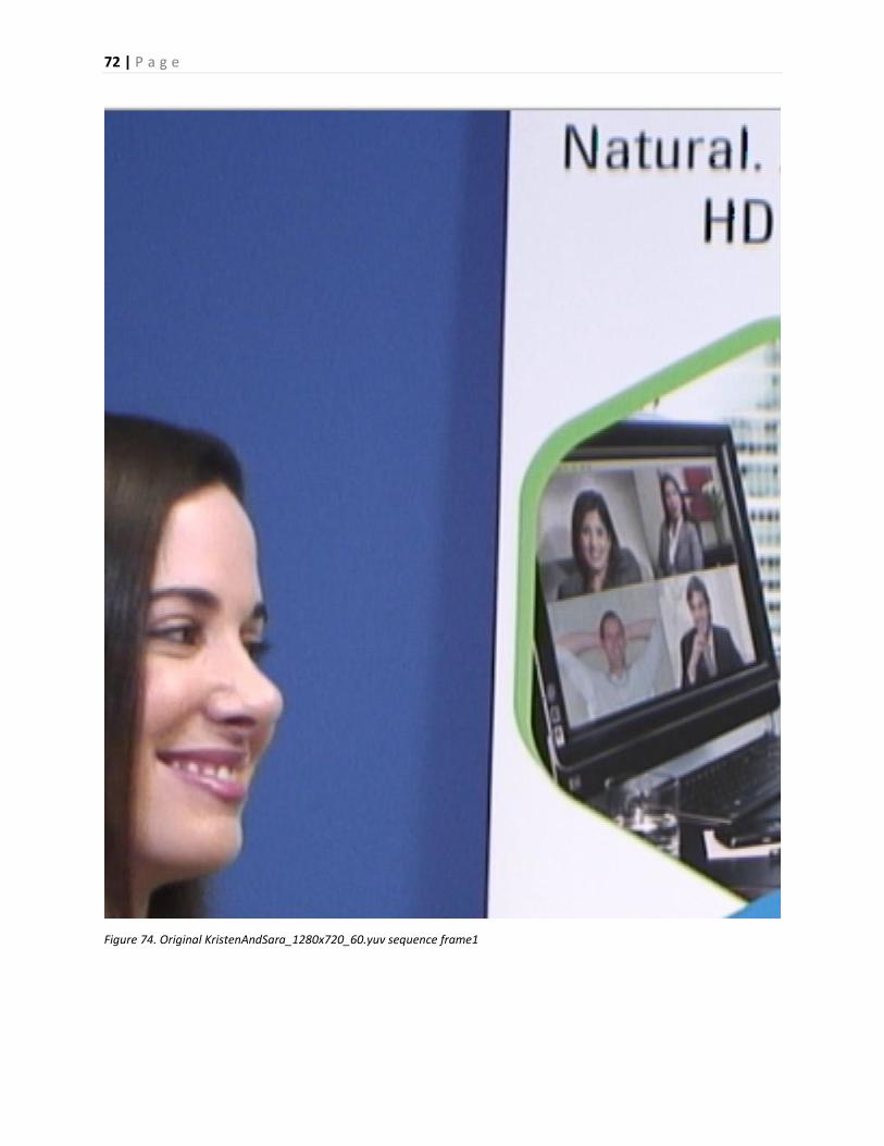
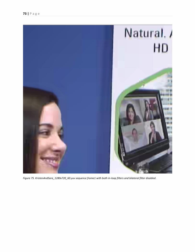
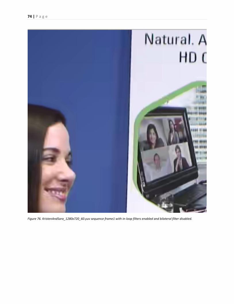
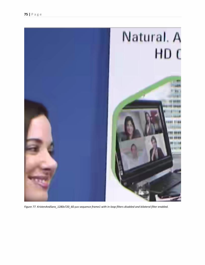
Figure 54. Performance of Deblocking filter in HEVC for KristenAndSara Drive Sequence [9]
Similarly, performance of HEVC SAO filter is shown in figures 56 and 57.
Figure 55. Performance of SAO filter in HEVC on SliceEditing sequence [9]
Figure 56. Performance of SAO filter in HEVC on RaceHorses sequence [9]
As, we can see from the figures 56 and 57, ringing artifacts are slightly reduced.
Even though HEVC greatly reduces the compression artifacts, there is still scope for improvement such
as ringing artifacts and this is the motivation toward my thesis.
53 | P a g e
Chapter 5 – Adaptive Bilateral Filtering to Remove Compression Artifacts Though HEVC employs in-loop filters such as deblocking and SAO filters to remove compression artifacts
due to block based coding and coarse quantization of transform coefficients, there is still a scope for
improvement. As in-loop filters are part of the standard, any modification of in-loop filters would modify
the coding standard. So, post-processing techniques have gained popularity as they would not disturb
the existing standard and reduce compression artifacts.
The current thesis focusses on applying bilateral filter on HEVC decoded frames adaptively to remove
compression artifacts and still maintain very good visual quality.
The bilateral filter discussed in chapter 4.3 is applied at each pixel of the frame. The bilateral filter
preserves the edges while smoothing the image. To apply bilateral filter in an adaptive way, we divide
the frame into 4x4 blocks and calculate sigma for spatial (σ s|) and intensity domains (σ r
|). First, each 4x4
block is categorized in to a strong edge, weak edge, texture or smooth block. This is done by
determining the standard deviation (STD) in a 4x4 block around each pixel [21] and then spatial sigma
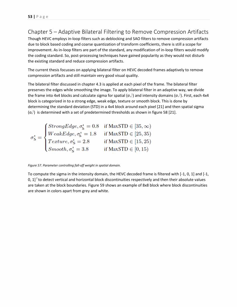
(σs|) is determined with a set of predetermined thresholds as shown in figure 58 [21].
Figure 57. Parameter controlling fall-off weight in spatial domain.
To compute the sigma in the intensity domain, the HEVC decoded frame is filtered with [-1, 0, 1] and [-1,
0, 1] T to detect vertical and horizontal block discontinuities respectively and then their absolute values
are taken at the block boundaries. Figure 59 shows an example of 8x8 block where block discontinuities
are shown in colors apart from grey and white.
54 | P a g e
Figure 58. Block discontinuity Map for 8x8 pixel block [22]
Applying block discontinuities on the edges does not remove compression artifacts completely and
hence it is applied on all the pixels by taking edge discontinuities along the block boundary and
interpolating remainder of pixels using bi-linear interpolation. The center 4 gray pixels are marked zero
before interpolation. After interpolating all the pixels in 8x8 block we get 8x8 discontinuity map. These
values are used as sigma in the intensity domain. Hence using the sigma values in the spatial and
intensity domain for each pixel, bilateral filter is applied and the results are shown in chapter 6.
55 | P a g e
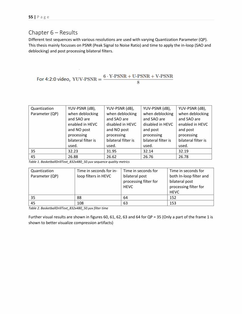
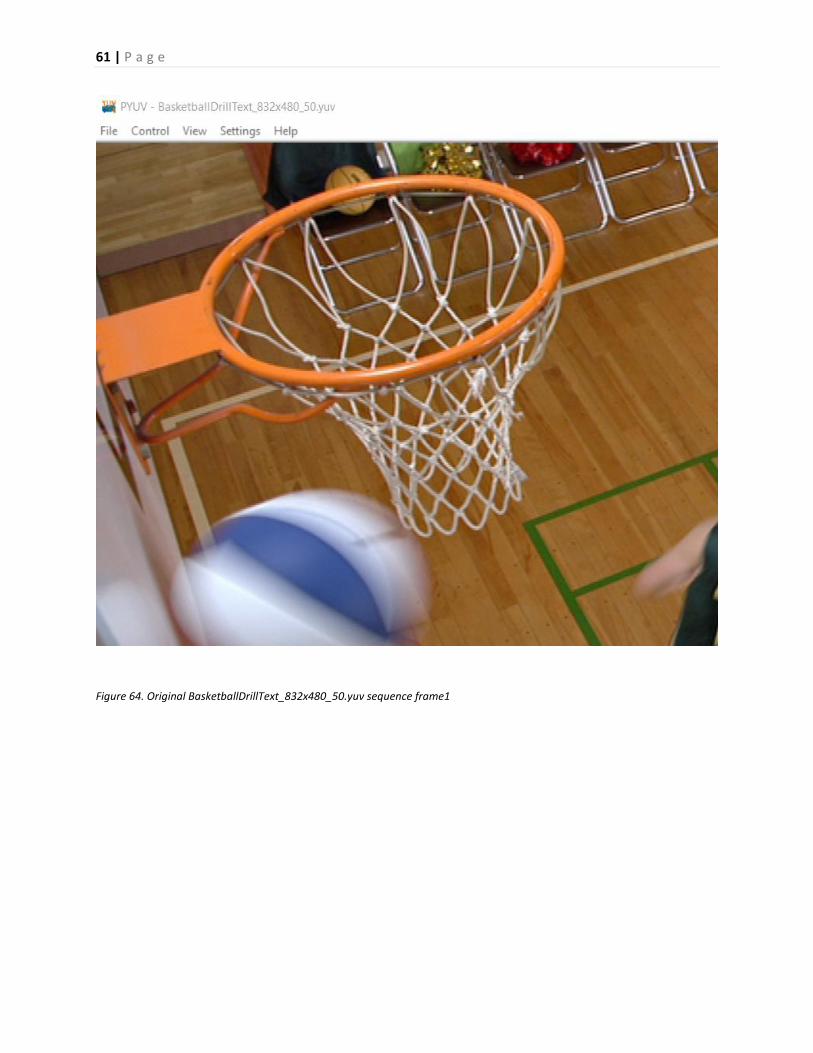
Chapter 6 – Results Different test sequences with various resolutions are used with varying Quantization Parameter (QP).
This thesis mainly focusses on PSNR (Peak Signal to Noise Ratio) and time to apply the in-loop (SAO and
deblocking) and post processing bilateral filters.
Quantization Parameter (QP)
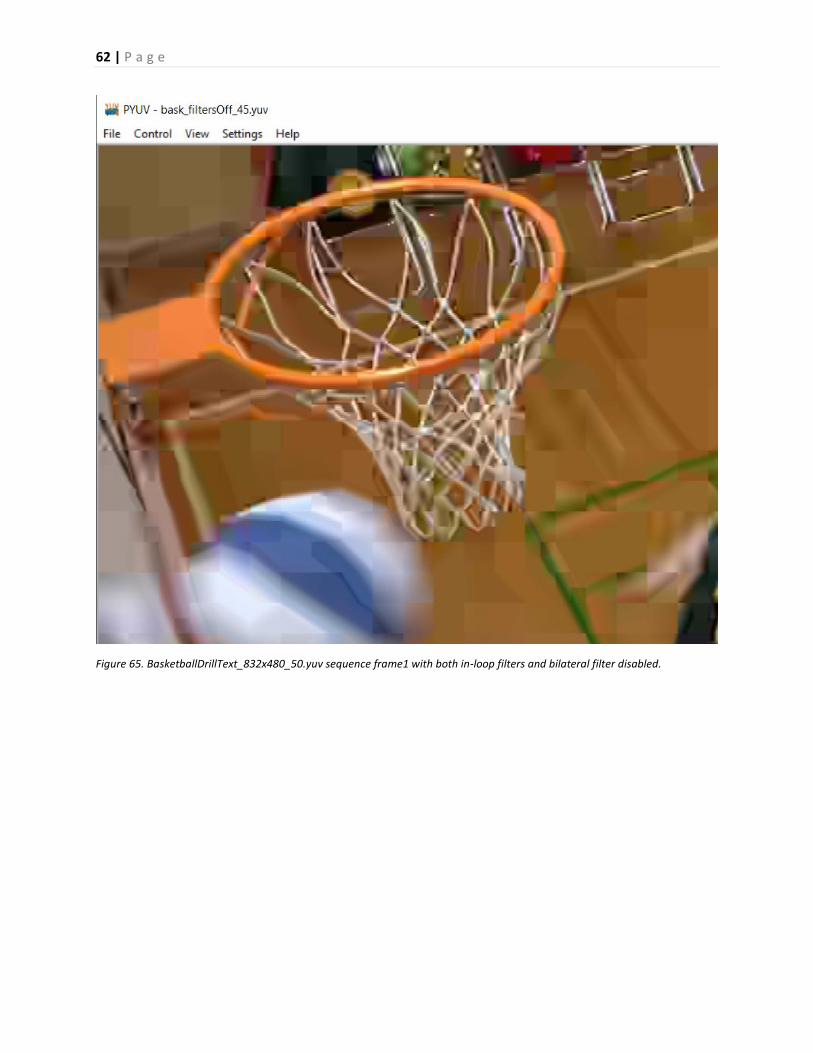
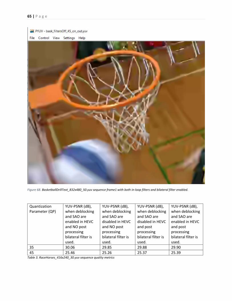
YUV-PSNR (dB), when deblocking and SAO are enabled in HEVC and NO post processing bilateral filter is used.
YUV-PSNR (dB), when deblocking and SAO are disabled in HEVC and NO post processing bilateral filter is used.
YUV-PSNR (dB), when deblocking and SAO are disabled in HEVC and post processing bilateral filter is used.
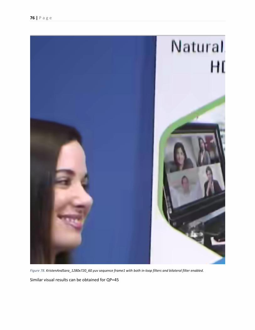
YUV-PSNR (dB), when deblocking and SAO are enabled in HEVC and post processing bilateral filter is used.