40
1 Part IV. Renewable Resources A. Fish – part 1: Biology and optimal harvest B. Forests C. Water D. Biodiversity
| Date post: | 19-Dec-2015 |
| Category: |
Documents |
| View: | 216 times |
| Download: | 2 times |

1
Part IV. Renewable Resources
A. Fish – part 1: Biology and optimal harvest
B. Forests
C. Water
D. Biodiversity

2
B. Fish
Chapter 11

3
Intro
• Modern fishing technology, coupled with increased demand and open-access exploitation of fisheries, has driven many fish stocks to such low levels that they are threatened with extinction.
• As illustrated in Table 11.1, fish populations are declining throughout the world.
• The proportion of global fish stocks that are in a state of decline has risen from 10% in 1975 to almost 30% in 2002.

4
MSY – max amount harvest year after year in a sustainable fashion. Exploitation beyond MSY leads to declining populations.

5
Intro
• Recreational fishing is also very important in the United States.
• According to the U.S. Fish and Wildlife Service, approximately 34 million adult Americans (over age 16) participated in recreational fishing in 2001.
• These anglers accounted for 500,000 days of fishing and $35 billion on fishing-related expenses.

6
Fisheries Biology
• The reproductive potential of a fish population is a function of both the size of the fish population and the characteristics of its habitat.
• Both the growth of the population and the population itself are measured in biomass (weight) units.
• Biomass does not distinguish between number of individuals and mass of individuals.
• Figure 11.1 depicts a logistic growth function which illustrates the relationship between the fish population and the growth rate of the population.

7
Initially, there is no growth, then over some range of population (up to X2), population growth is increasing. Beyond X2, the growth of the population is decreasing.
8
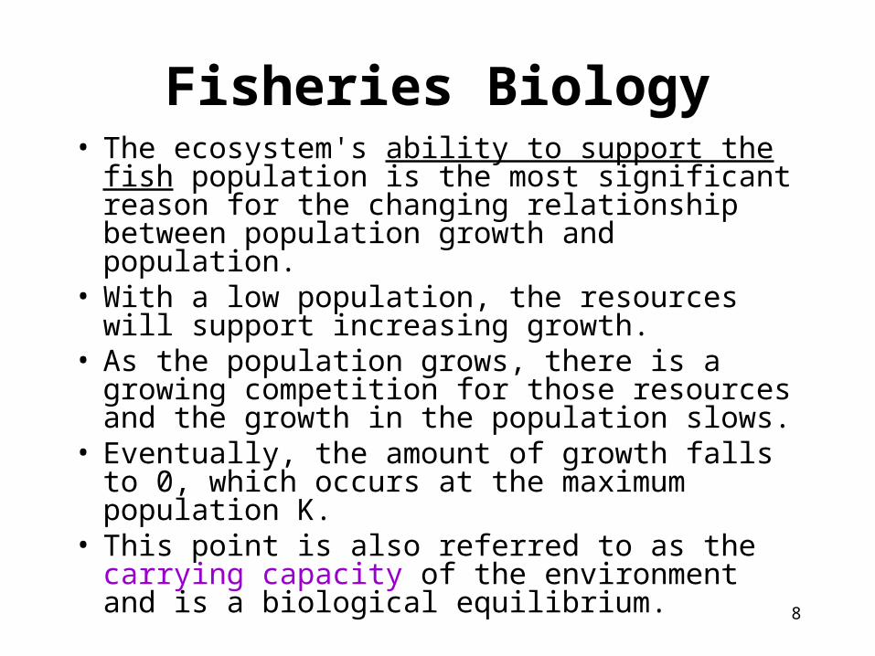
Fisheries Biology• The ecosystem's ability to support the fish
population is the most significant reason for the changing relationship between population growth and population.
• With a low population, the resources will support increasing growth.
• As the population grows, there is a growing competition for those resources and the growth in the population slows.
• Eventually, the amount of growth falls to 0, which occurs at the maximum population K.
• This point is also referred to as the carrying capacity of the environment and is a biological equilibrium.

9
11.2 represents a depensated growth function, where the growth rate initially increases and then decreases.
The logistic growth function represented in Figure 11.1 represents a compensated growth function (growth rate always declining).

10
• Fig.11.3 contains a critically depensated growth function where, X0 represents the minimum viable population. If population falls below this level, growth becomes negative and population becomes irreversibly headed towards 0.• The implication is that if managers make a mistake and allow too much harvest, they may doom the population to extinction.
11
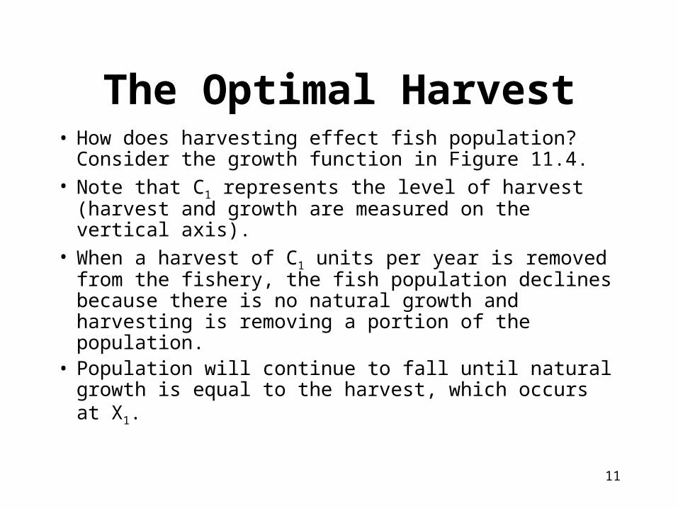
The Optimal Harvest• How does harvesting effect fish population? Consider
the growth function in Figure 11.4. • Note that C1 represents the level of harvest (harvest
and growth are measured on the vertical axis). • When a harvest of C1 units per year is removed from
the fishery, the fish population declines because there is no natural growth and harvesting is removing a portion of the population.
• Population will continue to fall until natural growth is equal to the harvest, which occurs at X1.

12

13
The Optimal Harvest
• In Figure 11.5 a harvest level of C1 is associated with two equilibrium populations (X1' and X1").
• This means that growth is exactly equal to harvest and the population will remain unchanged at either of these levels.
• Cmsy represents the harvest level associated with maximum sustainable yield (MSY) for the fishery.
• This is the only harvest level associated with 1 equilibrium point.

14

15
The Optimal Harvest
• In the early discussions of fishery management, MSY was the theoretical goal of management policies.
• Recent policy targets a more precautionary goal of keeping population between the carrying capacity and the level associated with maximum sustainable yield (harvest to left of MSY)
• Maximization of physical quantity will NOT necessarily maximize economic benefits.

16
The Gordon Model
• In a 1955 article, H. Scott Gordon made the point that uncontrolled access to fishery resources would result in a greater than optimal level of fishing effort.
• Gordon derived a catch function that represented a “bionomic” equilibrium.
• This catch function considered the relationship between fishing effort, catch, and fish population.
• Gordon’s analysis began by assuming that, holding everything else constant, catch is proportional to the fish population.

17
Figure 11.6 illustrates a set of yield functions, where each curve represents a different level of fishing effort.
Of course, not every point on each yield function is sustainable (growth = catch)
18
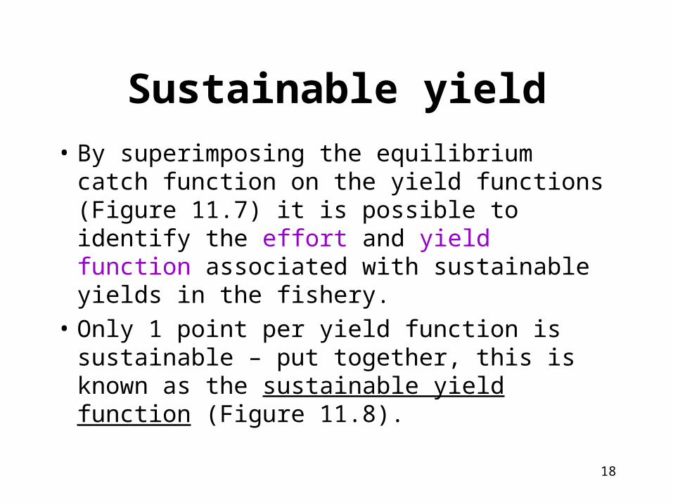
Sustainable yield
• By superimposing the equilibrium catch function on the yield functions (Figure 11.7) it is possible to identify the effort and yield function associated with sustainable yields in the fishery.
• Only 1 point per yield function is sustainable – put together, this is known as the sustainable yield function (Figure 11.8).

19
Superimposed equilibrium catch function on the yield functions – gives sustainable yields (catch=growth) at C1, C2, C3

20
The 1 point of sustainable catch associated with each level of effort is graphed with the corresponding level of effort on the x axis
As effort increases, sustainable yield increases and then decreases. Note order of C1, C2, C3.

21
Sustainable total revenue• A sustainable total revenue function can be derived
from a sustainable yield function.• Price is assumed to be constant, based on the additional
assumption that catch from that particular population will be small relative to the total market.
• Given a constant price, a sustainable total revenue function can be derived simply by rescaling Figure 11.8.
• In Figure 11.9, the sustainable total revenue function is labeled TR and an additional curve representing total costs (TC) is also given.

22
23
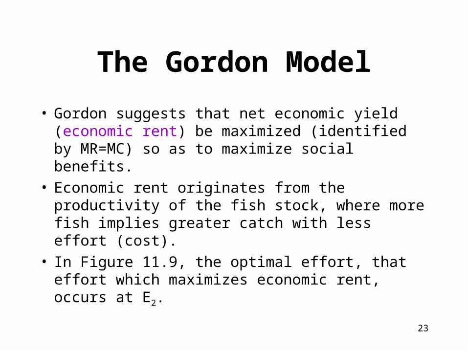
The Gordon Model
• Gordon suggests that net economic yield (economic rent) be maximized (identified by MR=MC) so as to maximize social benefits.
• Economic rent originates from the productivity of the fish stock, where more fish implies greater catch with less effort (cost).
• In Figure 11.9, the optimal effort, that effort which maximizes economic rent, occurs at E2.

24
The Gordon Model
• In an open-access fishery, when economic rent is earned in the fishery, entrance by new firms occurs until economic rent falls to zero, effort level of E1 in Figure 11.9.
• The entrance of firms in response to economic rent and the resulting increase in effort to E1 results in AR = MC rather than the optimal effort level of E2 where MR=MC.
• Table 11.2 illustrates the relationship between total catch, marginal catch, and average catch.

25

26
MR vs. AR
• Examine the 5th fisher in fishery• Adds $70 of catch to total, but actually catches
$78 of catch• If all fishers had same skill, catch same amount of
fish• Of $78, $70 = new catch, $8 would’ve been
caught by existing fishers• When fisher decides whether to enter fishery,
compares $78 to her opportunity cost (instead of $70)
27
Open access decisions
• Important because social efficiency requires MC = MR. Remember why?
• Unlike the behavior of a single firm operator, where the addition to output of an additional unit of input is measured by MR (catch) and compared to price, within the fishery there is not a single firm operator over the whole fishery.
• Each individual fisher compares their average catch and associated revenue (AR) with the value of the highest alternative to fishing.

28
Another example
• If opportunity cost of fishing $50 per day, then workers will continue to enter fishery as long as average catch > $50, which occurs at a level of effort of 12 fishers.
• At this point, the marginal catch of the 12th fisher is actually 0.
• The optimal level of effort occurs at 7 fishers, where marginal catch = opportunity wage

29
30
Too much effort
• The Gordon model is designed to focus on the inefficiency associated with open-access, and the loss in welfare associated with too much effort being employed in the fishery.
• Gordon suggests that a monopoly within the fishery would prevent the inefficiency associated with open-access.
• Policies based on Gordon’s suggestion of limiting effort within the fishery have been ineffective and brought many world fisheries to the brink of collapse. Why?

31
Shortcomings of the Gordon Model
• The primary shortcoming of the Gordon model is that it is static in nature, rather than dynamic.
• Clark (1985) shows that as the discount rate gets very large, the dynamically optimal level of catch approaches that associated with OA.
• Another shortcoming of the Gordon approach is that it does not consider CS and PS, which may exist and be important in many fisheries, particularly for some threatened fisheries such as salmon, redfish, and Alaskan King Crab.

32
Incorporating CS & PS in Fishery Models
• In an attempt to incorporate CS and PS into a model of the fishery, conventional demand and supply models are integrated into the fishery model (Figure 11.11). The horizontal axis is no longer measured in terms of effort, but in units of catch.
• F’s are populations (F1 > F2 > F3…)

33

34
Incorporating CS & PS in Fishery Models
• Figure 11.12 illustrates a family of supply functions, each defined for a different level of the fish stock.
• There are multiple equilibria, each associated with a different supply and demand interaction.
• However, for each level of population represented, there is only 1 sustainable level of catch.

35
Incorporating CS & PS in Fishery Models
• Figure 11.13 identifies the 6 sustainable catch levels (catch=growth), each associated with a different supply function (C1 – C6)
• These catch values are then identified on the supply curves in Figure 11.14. (combines 11.12 + 11.13) For example, the equilibrium catch associated with the max population of F1 is zero, which is identified as point A on Supply function SF1.
• Can you think of why this is?• Sustainable implies catch = growth. At max pop
(K), zero growth.

36

37
Incorporating CS & PS in Fishery Models
• Figure 11.15 illustrates the bioeconomic equilibrium. • It considers the intersection between demand, a supply
function and the biological equilibrium represented by a third backward bending curve.
• Equilibrium occurs at point E (all 3 curves intersect)• A sole owner of a fishery could locate at point F, which is
associated with a higher fish stock (easier to catch same amount).
• At point F, economic rent is equal to the area PEFB, consumers' surplus is the area PDE, and producers' surplus is the area BFA. (price and cost different here)
• At point E there would be no economic rent. This is consistent with an open-access fishery.

38
The objective of fishery management would be to choose a point along the sustainable catch curve that maximizes the sum of economic rent + consumer + producer surplus.

39
Pollution in Fishery Models
• It is also possible to use this model to examine other types of fishery management problems.
• An example would be modeling the fishery-related damages from the pollution in the Chesapeake Bay.
• Evidence suggests that there are strong locational advantages across potential fishing sites.
• This translates into an increasing marginal cost function associated with catching striped bass.
• The impact of pollution may be to decrease the carrying capacity of the environment.

40
The result is that the locus of points that illustrate the biological equilibrium associated with different supply functions has shifted inward (Figure 11.7).


