58


Regional Low-emission pathways
from global models
Deliverable 1.1 for the MILES project
MILES: Modelling and Informing Low-Emission Strategies
Heleen van Soest*1), Lara Aleluia Reis2), Detlef van Vuuren1),
Christoph Bertram3), Laurent Drouet2), Jessica Jewell4), Elmar
Kriegler3), Gunnar Luderer3), Keywan Riahi4), Joeri Rogelj4),
Massimo Tavoni2,5), Michel den Elzen1)
Aayushi Awasthy6), Katherine Calvin7), Pantelis Capros8), Leon Clarke7), Michel
Colombier9), Teng Fei10), Amit Garg11), Fernanda Guedes12), Mariana Imperio12),
Mikiko Kainuma13), Jiang Kejun14), Alexandre C. Köberle12), Peter Kolp4), Volker
Krey4), Alban Kitous15), Paroussos Leonidas16), Andre Lucena12), Toshihiko
Masui13), Larissa Nogueira12), Roberta Pierfederici9), Bert Saveyn15), Roberto
Schaeffer12), Fu Sha17), Bianka Shoai18), P.R. Shukla11), Thomas Spencer 9),
Alexandre Szklo12), Henri Waisman9)

1) PBL Netherlands Environmental Assessment Agency, The Netherlands
2) Centro Euro-Mediterraneo sui Cambiamenti Climatici (CMCC), Italy and
Fondazione Eni Enrico Mattei
3) Potsdam-Institut für Klimafolgenforschung (PIK), Germany
4) International Institute for Applied Systems Analysis (IIASA), Austria
5) Politecnico di Milano, Italy
6) The Energy and Resources Institute (TERI), India
7) Pacific Northwest National Laboratory (PNNL), United States
8) Institute of Communication and Computer Systems (ICCS), Greece
9) Institut du Développement Durable et des Relations Internationales
(IDDRI), France
10) Tsinghua University (TU), China
11) Indian Institute of Management Ahmedabad (IIMA), India
12) The Alberto Luiz Coimbra Institute for Graduate Studies and
Research, Federal University of Rio de Janeiro (COPPE/UFRJ), Brazil
13) National Institute for Environmental Studies (NIES), Japan
14) Energy Research Institute of NDRC (ERI), China
15) European Commission, DG Joint Research Centre (JRC), Spain
16) Energy - Economy - Environment Modelling Laboratory (E3M Lab),
Greece
17) Renmin University and National Centre for Climate Change Strategy
and International Cooperation, China
18) Research Institute of Innovative Technology for the Earth (RITE),
Japan
*Corresponding author: [email protected]

SUMMARY
The purpose of this paper is to synthesize and provide an overview of the
national and regional information contained in different scenarios from various
global models published over the last few years. We use this information to
analyse the emission reductions and related energy system changes in various
countries in pathways consistent with the 2oC target. This analysis provides input
for international policy processes, and the context for more detailed analyses of
meaningful indicators at the national level. We note that although we present the
results of several models, these are used to build significant corridors and not as
a basis for an inter-model comparison, which is not the scope of this work.
In our work, the scenarios were characterized on the basis of the assumed
climate policies: i.e. baseline scenarios (no new policies), reference scenarios
(existing policies) and scenarios aiming at 550 and 450 ppm CO2-eq targets. The
latter were divided into scenarios with and without assumed delay in policy
implementation in the near term. Each of the global models contains information
for about 10-30 regions and countries. The scenarios with delay implement
prescribed policies per region. After the delay period, a uniform global carbon
price is assumed. This implies that the contribution of each country (or region) is
mostly determined by the marginal abatement costs. This is also the case for the
scenarios without delay for the full scenario period. Differences in model
outcomes have been used to indicate model uncertainty ranges for the various
indicators that are shown.
Emission trends
In this summary, we focus on the baseline and 450 ppm CO2-eq scenarios (see
Box 1).
Box 1: Model-based scenario analysis The baseline scenario shows the situation in the absence of climate policy. Such
a scenario is not realistic (as most countries have indicated elaborate plans to implement policies), but forms a counterfactual scenario that can be used to show the effect of policies in each region in a compatible way. For the 450 ppm
scenarios, two categories are shown, i.e. with and without delay. The scenarios without any policy delay are also not realistic, but again, provide a reference
showing the situation if a globally cost-efficient response could be formulated. In the database, results from various models were available for 13 regions.
Models provide insights into cost-optimal trajectories for achieving specific climate goals given assumptions on the costs, efficiency and preferences for
specific technologies, their interaction in the energy system and existing policies.

The information can be used to explore costs and benefits of alternate pathways. Future policy developments are beset with uncertainty. The use of multiple models is one way to obtain some insights into the impact of different model
assumptions.
Figure S.1 shows the mean values of projected trends in per capita GDP levels
and associated per capita emissions for all models (baseline and 450 ppm CO2-
eq) for 13 regions covered in this study. This figure leads to the following
conclusions:
Without climate policy, greenhouse emissions are expected to
increase rapidly in low-income regions, driven by a projected
further increase in economic activity and population. Per capita
emissions are projected to remain more or less stable in high-
income regions. The emissions per capita in high-income countries are
expected to remain more or less stable as a result of opposing trends in
activity growth, efficiency improvement and (slow) decarbonisation of fuel
supply.
Emissions in the mitigation scenarios are significantly reduced
compared to the baseline in all regions, independent of income-
level. Further analysis of the scenarios shows global average CO2
emissions to range from about 0.3 to 2 tCO2/capita in 2050 under delayed
450 scenarios. This range results from differences in non-CO2 emissions
assumptions and assumed mitigation action beyond 2050 (especially the
use of negative emissions). Figure S.1 shows that low-income countries
generally remain below the global average, although the upper end of the
ranges for China, Indonesia and South Africa are slightly above the global
average. Most OECD countries show per capita emissions ranges similar to
or higher than the global average.
The results also show that CO2 emissions from fossil fuels and
industry represent the majority of global total emissions in the
baseline, while the mitigation scenarios result in about equal
shares of non-CO2 emissions and CO2 emissions from fossil fuels
and industry globally in 2050. CO2 emissions are reduced more than
non-CO2 emissions. There are, however, regional differences in the
contribution of the different emission categories. In China, for example,
CO2 emissions from fossil fuels and industry remain the major contributor
to total emissions, while in Indonesia, land use emissions represent the
lion’s share. All countries show increasing shares of low-carbon primary
energy sources (i.e. all energy sources except coal, oil and gas without
carbon sequestration) with lower cumulative carbon emissions. For
developed countries, this generally means a substantial increase on 2010
levels.

Figure S.1: CO2 emissions per capita (tCO2/capita) versus GDP per capita (US$2005/capita) between 2010 and 2050 for baseline scenarios (left panel) and cost-optimal 450 scenarios (right panel).
Greenhouse emissions in 2030
The results across the different models for 2030 greenhouse gas emissions are
summarized in Figure S.2.
The data show a clear difference in 2030 emission levels between
the baseline scenarios and the cost-optimal 450 ppm scenarios.
The delayed 450 ppm scenarios typically show slightly higher emissions
than the cost-optimal 450 ppm scenarios.

Figure S.2: Kyoto gas emissions (MtCO2e) in 2030 for cost-optimal 450 ppm scenarios, delayed 450 ppm scenarios and baseline scenarios. Filled bars show the median value across models, error bars show the 10th to 90th percentile range.
Cumulative emissions
A key outcome of the models are the regional cumulative emissions
consistent with different global climate targets. These can be interpreted as
regional emission constraints assuming cost-efficient implementation of the
global target across all regions. Note that the cumulative emissions linked to e.g.
a <2°C temperature outcome need to be constantly updated to account for
revised estimates of past, current and future emissions as well as developments
in climate science.
Figure S.3 shows the regional cumulative emissions for the baseline and
optimal 450 scenarios for the period 2010-2100. The results indicate the
actual emissions in the cost-optimal scenarios and do not make any
assumptions as to who pays for the emission reductions. The cumulative
emissions between the baseline and 450 scenario are very
different, showing on average around 76% reduction across all
regions. The important role of China, India, and the USA is illustrated by
the fact that in the baseline scenario, each of these regions alone accounts
for at least half the global cumulative emissions consistent with the 2oC
target. The different ratios between baseline emissions and the cost-
optimal 450 emissions mostly reflect abatement opportunities in the
various regions.

Figure S.3: Regional cumulative CO2 emissions between 2010 and 2100, for cost-optimal 450 ppm
and baseline scenarios. Filled bars represent the median, error bars give the 10th to 90th percentile ranges across models.
Emissions peak
A similar picture of stringent climate action in all regions emerges when
looking at the peak year of CO2 emissions (Figure S.4). Under the optimal
450 scenarios that assume direct implementation of policies, most
countries’ CO2 emissions peak before 2025 (except for India). Under
delayed 450 scenarios (taking into account 2020 pledges and introducing
cost-optimal policies between 2020 and 2025), this peak generally shifts
to later in the century, although not by much.

Figure S.4: Regional peak years of CO2 emissions for cost-optimal 450 ppm, delayed 450 ppm and
baseline scenarios. Dots give the median of the models, error bars give the 10th to 90th percentile ranges. The median results can be at the outer end of the range, for instance for OECD countries, as a majority of these regions show an immediate peak with only a few exceptions.
Consequences for energy use
Primary energy demand decreases strongly in the mitigation scenarios,
compared to the baseline scenario, especially in developing countries. The
450 scenarios show a reduction in all countries of roughly 30-40%
compared to the baseline. There are regional differences, with e.g.
South Africa halving its primary energy demand under mitigation
scenarios.
Key differences between the baseline scenario and the 450 ppm
scenario occur for the composition of the energy mix (Figure S.5). In
the baseline scenario, the contribution of low-carbon energy technology
remains around 15%, i.e. similar as today. Large differences across the
different regions can be seen in the baseline projections for 2030 and
2050, with Brazil showing significantly higher shares of low-carbon energy
technology than other regions. In the mitigation scenario, the shares of
low-carbon energy technology are scaled up rapidly towards 2050. While
some differences across the regions can be noticed, the large model
uncertainty ranges indicate that this differs strongly across the models.
Policy costs
There is a cost advantage to starting mitigation early. Delayed 450
scenarios show lower median policy costs in the short term in some
regions (China and World), but higher policy costs in the long term in all
regions, compared to the optimal 450 scenarios.
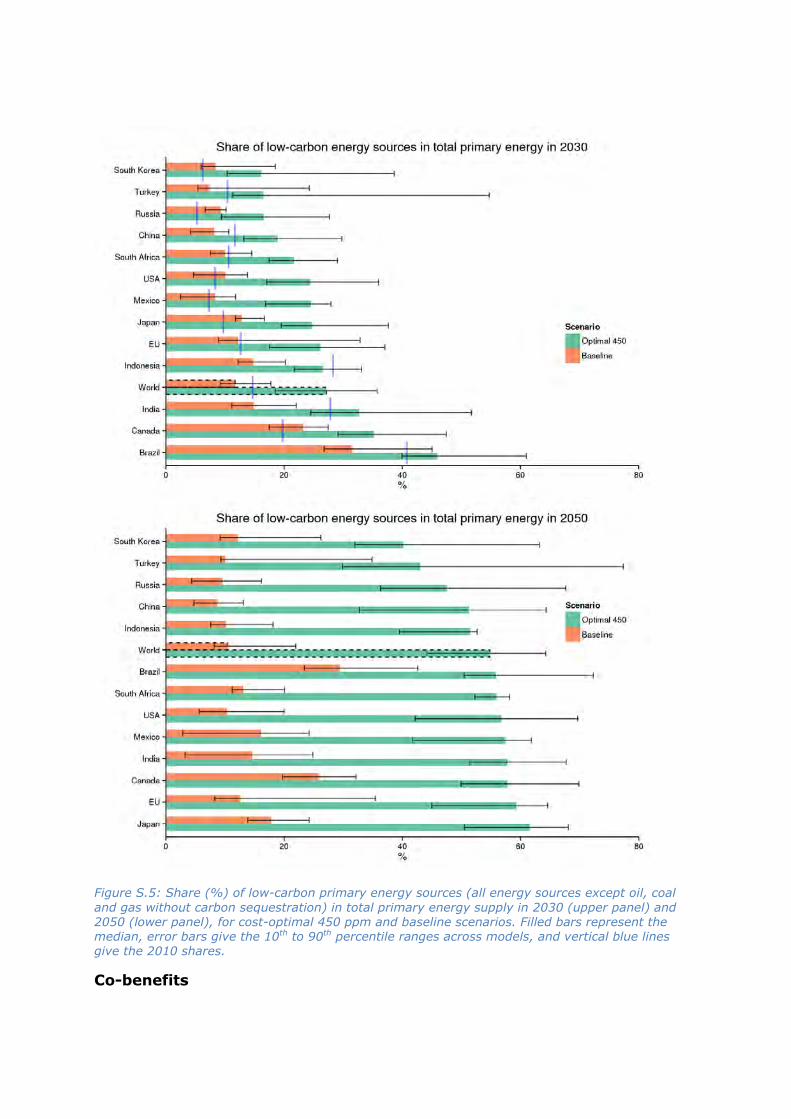
Figure S.5: Share (%) of low-carbon primary energy sources (all energy sources except oil, coal
and gas without carbon sequestration) in total primary energy supply in 2030 (upper panel) and 2050 (lower panel), for cost-optimal 450 ppm and baseline scenarios. Filled bars represent the median, error bars give the 10th to 90th percentile ranges across models, and vertical blue lines give the 2010 shares.
Co-benefits

Mitigation action does not only impact greenhouse gas emissions, but also the
energy mix – and thus energy security and air pollution. Overall, it has been
shown on the global level that mitigation action is likely to result in co-benefits.
The analysis here shows such co-benefits for air pollution (although showing
clear regional differences), but for energy security, the impacts of mitigation
action are dependent on the region.
Looking at air quality, sulphur dioxide emissions are strongly
reduced as a co-benefit of greenhouse gas emission reductions, in
both developing and developed countries (Figure S.6). Also significant
reductions of black carbon emissions can be found, although
emissions increase in countries that strongly rely on bioenergy to reach
mitigation targets. In these cases, additional policies are required to
reduce air pollution from black carbon.
Figure S.6: Changes, in 2050, in black carbon (brown) and sulphur dioxide (orange) emissions when moving from a baseline without new climate policies to a pathway in line with stabilizing atmospheric CO2-equivalent concentrations at 450 ppm. Dots show single model results, bars the full range.
Concerning energy security, energy importing countries generally
experience a decrease in net-energy imports in climate stabilization
scenarios compared to the baseline development, while energy exporters
experience a loss of energy export revenues from climate stabilization
policies (Figure S.7).

Figure S.7: Change in net-energy imports (left) and net-energy exports (right) for major energy importers and exporters. The number for each country represents the number of models.

Contents
INTRODUCTION 13
METHODOLOGY 15
Main Method 15
Regional Coverage of the Models 17
RESULTS 21
Population and GDP 21
Primary Energy 24
Energy Intensity 26
Greenhouse Gas Emissions 27
Emissions: CO2 Energy, CO2 Land Use, Non-CO2 31
Regional cumulative emissions 33
Peak Year 34
Low-carbon energy technology as a function of cumulative emissions 35
Policy Costs 39
Implications of Technology Availability Assumptions 40
Co-benefits 42
Energy Security and Energy Independence Co-benefits of Mitigation 42
Air Pollution Co-benefits of Mitigation 45
CONCLUSIONS 47

Introduction
Governments worldwide have agreed that international climate policy should aim
to limit the increase of global mean temperature to less than 2oC with respect to
pre-industrial levels (UNFCCC, 2010). The IPCC Fifth Assessment Report (AR5)
indicates that scenarios without new climate policies typically result in a an
increase of global mean temperature of around 3-4°C by 2100 (Clarke et al.,
2014). In order to reach the 2oC target, urgent and drastic emission reductions
are required. Such reductions are needed in all regions around the world (Tavoni
et al., 2014).
Global modelling teams have worked on developing a set of scenarios for
international climate policy in projects such as AMPERE (Kriegler et al., 2014a),
LIMITS (Kriegler et al., 2014b, Riahi et al., 2014, Tavoni et al., 2014) and EMF27
(Kriegler et al., 2014c). These scenarios look into possible emission trajectories
without new climate policies, estimates of current policies and different variants
of scenarios aiming at the 2oC target (these scenarios vary in terms of the
probability of achieving the target, technology assumptions and the timing of
climate policy). The scenarios also played an important role in the analysis
performed in the last report of IPCC (Clarke et al., 2014). Typically, these models
contain around 10–30 regions in order to describe trends in global emissions.
While several projects have started to use the regional information of the global
models to look into climate policy strategies at the scale of countries and regions
(e.g. Herreras Martínez et al., 2015, Tavoni et al., 2014, Van Sluisveld et al.,
2013), in general, the regional information has not been used extensively.
The purpose of this paper, therefore, is to analyse the energy system changes in
various countries in pathways consistent with the 2oC target, by looking into the
national/regional information contained in different global scenarios from various
global models. The objectives of this study are:
To better understand the transition pathways at the level of major
economies in a set of global scenarios developed over the past few years;
To specifically investigate various policy relevant indicators such as peak
years and cumulative emissions at the level of major economies;
To provide insights in potential co-benefits of different pathways.
The information presented here was evaluated by both national and international
modelling teams. This analysis could in particular help positioning the different
countries regarding low-emission pathways. The focus of the analysis is on
regional results (and thus not on a model comparison).


Methodology
Main Method
In this paper, we compare scenarios developed in previous studies using global
models in terms of the results for key countries/regions. We use data from the
following studies: AMPERE, LIMITS, and EMF27 (see earlier references), which
include several models such as DNE21+, GCAM, GEM-E3, IMAGE, MESSAGE,
POLES, REMIND, and WITCH.
In addition, new scenarios, developed after these previous studies or specifically
for the MILES project, have been added by the teams participating in MILES. The
MILES project (Modelling and Informing Low Emission Strategies) is an
international cooperation project between 19 international research teams1. Key
objectives of the project are: 1) to explore different country-level strategies
consistent with the 2oC target, 2) to increase understanding of differences
between strategies in different parts of the world, and 3) to enhance in all
participating countries the capacity to perform analysis of mitigation strategies.
In this study, we look into regional results evaluating the drivers, emission
trajectories, and energy system changes. The national and regional emission
pathways in the global studies provide insight into the required energy
transitions at this level. It should be noted that in these studies, the contribution
of each country (or region) in global reductions is determined by the marginal
abatement costs. The results of the global models have been compared with the
results of the national models.
The discussion of the results is divided into three parts, each of them oriented at
the following key questions:
What do regional/national emission and energy system pathways
consistent with different assumptions on international climate policy look
like?
How do assumptions on the availability of different technologies influence
these results?
What are important co-benefits at the national/regional level of the
different policies?
For this analysis, existing scenarios were characterized as indicated in Table 1.
1 ERI, RUC, TU, TERI, IIM, COPPE, PNNL, NIES, RITE, ICCS, IIASA, PIK, PBL, CMCC, CLU, IDDRI, CCROM, CRE, INECC


Table 1: Scenario categories used in this study.
Category Description
Baseline Scenarios that do not include new climate policies other than via the calibration to the historical period. This scenario category thus acts as a counterfactual
scenario providing a consistent reference across all regions for showing the impact of climate policies.
Reference policy Describes possible development assuming implementation of existing policies and some
continuation of these policies in the longer term (without strengthening these policies).
Cost-optimal 500-550 ppm CO2eq
Scenarios aimed at stabilizing GHG concentrations at the level of 500-550 ppm CO2-eq at the lowest costs (within the model).
Cost-optimal 450 A universal global carbon tax is implemented immediately in order to research a target of 450 ppm
CO2eq, resulting in the lowest costs (within the model).
Intermediate 450 This scenario type follows the implementation of the pledges in 2020 and assumes cost-optimal policies
(based on intermediate policies) to be introduced after 2020-2025.
Delayed 450 ppm CO2eq Scenarios that include the current description of pledges until 2020, and assume some further delayed policies up to 2025. In the longer term, cost-optimal
policies are implemented. As a result, global emissions peak after 2025.
Regional Coverage of the Models
Table 2 indicates how the information of the different models was used in this
study to look into regional trends. Table 3 provides the main characteristics of
the models included in this study.

Table 2: Regional coverage per model (X indicates that the region is represented in the model; in
case slightly different regions were used this is indicated in the Table).
DNE21+ GCAM GEM-E3 IMAGE MESSAGE POLES Remind WITCH
Brazil X X X X X
Canada X X X X X
China X Includes Hong Kong
X Includes Hong Kong, Macau
X Includes Hong Kong, Macau
X Includes Mongolia and Taiwan
X Centrally planned Asia and China
X Includes Hong Kong, Macau, Taiwan
X Includes Hong Kong
X
EU X Includes Greenland
X X Includes Norway, Switzerland, Iceland, Balkan countries
X Includes Iceland, Turkey, Norway, Switzerland, Greenland
X X X Includes EFTA
India X X X X X South Asia
X X X
Indonesia X X X X
Japan X X X X X X
Mexico X X X X X
Russia X X X X X X
South Africa
X X X X
South Korea
X X X Includes North Korea
X
USA X X Includes Puerto Rico
X X X North America (includes Canada, Guam, Puerto Rico)
X X Includes Puerto Rico
X
World X X X X X X X X
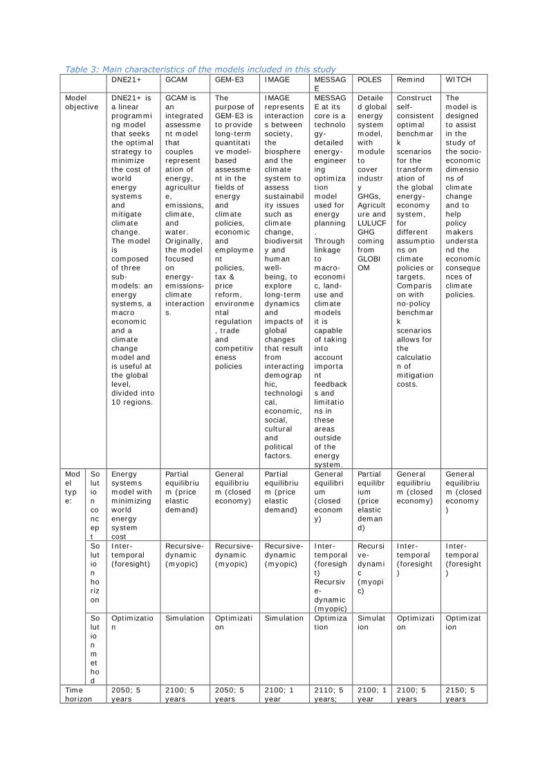
Table 3: Main characteristics of the models included in this study
DNE21+ GCAM GEM-E3 IMAGE MESSAGE
POLES Remind WITCH
Model objective
DNE21+ is a linear programming model that seeks the optimal strategy to minimize the cost of world energy systems and mitigate climate change. The model is composed of three sub-models: an energy systems, a macro economic
and a climate change model and is useful at the global level, divided into 10 regions.
GCAM is an integrated assessment model that couples representation of energy, agriculture, emissions, climate, and water. Originally, the model focused on energy-emissions-climate interactions.
The purpose of GEM-E3 is to provide long-term quantitative model-based assessment in the fields of energy and climate policies, economic and employment policies, tax & price reform, environmental regulation
, trade and competitiveness policies
IMAGE represents interactions between society, the biosphere and the climate system to assess sustainability issues such as climate change, biodiversity and human well-being, to explore long-term dynamics and impacts of
global changes that result from interacting demographic, technological, economic, social, cultural and political factors.
MESSAGE at its core is a technology-detailed energy-engineering optimization model used for energy planning. Through linkage to macro-economic, land-use and climate models it is
capable of taking into account important feedbacks and limitations in these areas outside of the energy system.
Detailed global energy system model, with module to cover industry GHGs, Agriculture and LULUCF GHG coming from GLOBIOM
Construct self-consistent optimal benchmark scenarios for the transformation of the global energy-economy system, for different assumptions on climate policies or targets. Comparison with no-policy benchmark
scenarios allows for the calculation of mitigation costs.
The model is designed to assist in the study of the socio-economic dimensions of climate change and to help policy makers understand the economic consequences of climate policies.
Model type:
Solution concept
Energy systems model with minimizing world energy system cost
Partial equilibrium (price elastic demand)
General equilibrium (closed economy)
Partial equilibrium (price elastic demand)
General equilibrium (closed economy)
Partial equilibrium (price elastic demand)
General equilibrium (closed economy)
General equilibrium (closed economy)
Solution horiz
on
Inter-temporal (foresight)
Recursive-dynamic (myopic)
Recursive-dynamic (myopic)
Recursive-dynamic (myopic)
Inter-temporal (foresight) Recursive-
dynamic (myopic)
Recursive-dynamic (myopic)
Inter-temporal (foresight)
Inter-temporal (foresight)
Solution method
Optimization
Simulation Optimization
Simulation Optimization
Simulation
Optimization
Optimization
Time horizon
2050; 5 years
2100; 5 years
2050; 5 years
2100; 1 year
2110; 5 years;
2100; 1 year
2100; 5 years
2150; 5 years

and time step
(2005-2030); 10 years (2030-2050)
10 years
Number of energy conversion technologies (rough estimate)
50 50 10 50 200 100 60 25
Energy technology substitution
Linear choice (lowest cost)
Logit choice model
Production function
Logit choice model
Linear choice (lowest cost)
Logit choice model
Production function
No discrete technology choices

Results
What do regional/national emission and energy system pathways
consistent with different assumptions on international climate policy
look like?
We selected a set of variables, presented hereafter, which are relevant for the
analysis of national emission and energy system pathways consistent with the
2°C target. The selection includes: population, GDP, primary energy demand,
energy intensity, GHG emissions, cumulative emissions, peak years, shares of
low-carbon energy sources, and policy costs.
Population and GDP are two important socio-economic drivers that have a direct
influence on primary energy demand and GHG emissions. The energy intensity
variable is a measure of the energy use per unit of economic activity and informs
about the general level of efficiency of a given region. Another widely used
indicator is cumulative emissions, which correlates well with the temperature at
the end of the century. The study of peak years allows us to compare countries
in terms of stringency of emission pathways. The shares of low-carbon energy
sources show the transitions needed in energy systems to meet the long-term
climate target. Finally, policy costs are relevant in this study in order to address
the regional impacts of delaying optimal mitigation.
Population and GDP
Figure 1 and Table 4 show the population and GDP per capita projections for the
different countries. Assumptions on the trends in these drivers do not vary
across different scenario categories.
The global population growth in the 2010–2050 period is projected to be about
30–40%. The GDP per capita growth over the same period is considerably faster
and the range in the assumed GDP growth across models is large for individual
regions, but also for the projected global GDP growth (i.e. 110–210%).

Table 4: Projected change in population and GDP per capita per region between 2010 and 2050
(2050 values expressed relative to 2010). UN population projections (medium variant) are also included for reference.
Region Population Population (UN medium)
Population (national scenarios)
GDP per capita
GDP per capita (national
scenarios)
Brazil [1.12, 1.19] 1.18 1.11 [2.53, 5.35] 3.14
Canada [1.29, 1.33] 1.33 [1.69, 1.87]
China [0.97, 1.07] 1.02 [4.91, 10.53]
EU [1, 1.05] 0.96 1.05 [1.77, 2.22] 1.71
India [1.33, 1.45] 1.34 [6.29, 14.65]
Indonesia [1.24, 1.34] 1.34 [4.82, 10.68]
Japan [0.81, 0.86] 0.85 0.80 [1.72, 2.19] 1.75
Mexico [1.17, 1.33] 1.32 [2.78, 4.01]
Russia [0.85, 0.91] 0.84 [2.44, 4.45]
South
Africa [1.13, 1.24] 1.23
[3.28, 5.48]
South Korea [0.91, 1.06]
1.05 [2.36, 2.79]
USA [1.28, 1.3] 1.28 [1.25, 1.88]
World [1.33, 1.39] 1.38 [2.09, 3.12]
Population growth
The projected population growth rates of the OECD countries lie well below the
global average. The populations of Japan and the Russian Federation are
projected to fall. In general, the different global model-based scenarios do not
include a very wide range of population projections, and agree well with UN
population projections. A notable exception is the EU, which shows slightly higher
population projections than the UN medium scenario. A key reason is that some
models include more countries in their EU region than the 28 EU member states
(e.g. Turkey, Greenland or Iceland).
The projected population growth rate of the low-income countries covered in this
study also lies below the global average. Again, the regional model projections
correspond well with the UN medium scenario, with a relatively small range
across the different models. The projected global average population growth rate
is higher than the growth rates of all countries covered in this study (except
India) due to high growth rates in other regions not covered here, most notably
Africa, and India.
Comparison with the national model results
The projections for Brazil are similar to the population projections by the national
modelling team. The Brazilian population is projected to reach around 200 million

inhabitants by 2030 and 230 million by 2050, which is based on the official
projections by the Brazilian Institute of Geography and Statistics (Herreras
Martínez et al., 2015). The projections for Mexico are in line with the findings by
Veysey et al. (2015), reporting on The Climate Modeling and Capacity Building in
Latin America project (CLIMACAP) and the Latin American Modeling Project
(LAMP). They project the Mexican population to reach about 150 million by 2050,
with MILES projections for Mexico reaching about 125 – 175 million.
GDP growth
GDP per capita is projected to increase in all countries. Again, the average of the
OECD countries lies significantly below the global average – although here Russia
forms an exception. The projected increase of other OECD countries is around 1–
1.7% per year, while the Russian growth included in the projections is 2.3-3.8%
per year.
The projected growth rate of the non-OECD countries is more than twice as high
as in OECD countries. The average growth rate of GDP per capita between 2010
and 2050 is projected to be around 3-6% per year in non-OECD countries, and
up to 4.7-6.8% per year for India.
Comparison with the national model results
Growth rates projected by the Indian team are slightly higher than most global
model projections (around 6.5% per year). Also the Brazilian national team’s
GDP projections were higher than those of (most of) the global models, with a
growth rate of 2.3–3.5% in the 2010-2030 period. These national GDP
projections are based on the Brazilian long term National Energy Plan, which
projects an average GDP growth of 4% per year until 2050. Mexico’s GDP in the
global model projections reaches a level of about US$ 2 – 4 trillion by 2050,
which is the same as the range reported by Veysey et al. (2015).

Figure 1: Population and GDP per capita in the 12 countries + world, relative to 2010 values. The
number of models per country reporting these variables is indicated2. No scenario category dimension is shown here, as assumptions on trends in drivers do not vary across scenario categories. Solid black lines show UN population projections (medium variant), solid blue lines show available national scenario projections.
Primary Energy
Primary energy demand projections under baseline, delayed, intermediate, and
optimal 450 scenarios are shown in Figure 2 (delayed and intermediate 450
scenarios are combined into one category). Primary energy demand decreases
strongly in the mitigation scenarios compared to the baseline scenario. This
2 Some regions and variables may show a larger number of models than the eight reported in Table 2, because models exist in different versions and with results of various studies in the database; these different model versions are
counted individually.

effect is strongest in developing countries. For most countries, the scenarios
from the global models encompass the IEA’s World Energy Outlook projections.
The largest difference can be observed in China. Here baseline results are quite
comparable, but the models show an outcome range for the optimal 450
scenarios that lies significantly below the IEA’s 2oC scenario. This may be
explained by the different accounting methods for total primary energy supply
applied by the IEA and official Chinese statistics. The Figure also emphasises the
considerable model uncertainty ranges for individual countries in the scenarios in
the literature.
OECD countries
In general, the primary energy projections for the OECD countries under baseline
assumptions show relatively small changes over time (increase or decrease). The
projections for the 450 scenarios show typically a 30-40% reduction compared to
the baseline scenarios by 2050.
Non-OECD countries
In baseline scenarios, the primary energy demand is projected to increase
strongly in most of the non-OECD countries. In contrast, the 450 scenarios show
a reduction of roughly 30-40% compared to the baseline by 2050, the same
order of magnitude as the reduction in the OECD countries. There are regional
differences, with e.g. South Africa showing a reduction up to 50% between the
baseline and the delayed + intermediate 450 scenarios.
Comparison with the national model results
Compared to national projections, not all global models show a similar reduction
of Indian energy demand (implying that the IEA scenarios are closer to the
national scenario projections than some of the global model projections). The
global model projections for Brazil are slightly lower than the projections by the
national modelling team. Primary energy demand is projected to be about 15 EJ
by 2050 under the intermediate 450 scenario in the global models, compared to
20 EJ according to the national model, which used the same carbon tax to create
a scenario similar to the ones developed by the global models. For the delayed
450 scenario, the Brazilian national model projection shows a slightly different
trajectory but a similar total primary energy demand in 2050 (about 40 EJ).

Figure 2: Total primary energy demand (EJ/year) in baseline, delayed + intermediate 450 ppm,
and optimal 450 ppm scenarios. IEA World Energy Outlook scenarios (450 ppm, current policies, new policies) are also plotted for reference. The number of models per country reporting this variable is indicated. Coloured vertical bars show the 2050 scenario ranges.
Energy Intensity
Primary and final energy intensity decrease strongly in all countries and all
scenarios, including the baseline scenario, but especially in developing countries
and the Russian Federation (Figure 3).
Comparison with the national model results
The projected trends in energy intensity are generally in line with national
scenario projections. For Brazil, the pathways as well as the absolute values are

very similar to the projections by the national modelling team. The Indian team
noted that the projected trend of declining energy intensity agrees with their
results of decoupling of energy use and GDP growth, although rates of
decoupling might differ. Veysey et al. (2015) expect some improvement in
energy intensity in Mexico between 2010 and 2020, and substantially more
improvement towards 2050. This trend is most pronounced in the delayed +
intermediate 450 scenarios shown in Figure 3.
Figure 3: Primary energy intensity (EJ/billion US$2005) in baseline, delayed + intermediate 450 ppm, and optimal 450 ppm scenarios. The number of models per country reporting the variables used to calculate energy intensity is indicated.
Greenhouse Gas Emissions

Figure 4 gives projected total CO2 emissions, while Figure 5 presents projected
CO2 emissions per capita. Worldwide, a strong emission increase can be observed
in the baseline scenarios, mostly driven by the trend in low-income countries. In
contrast, total CO2 emissions decrease rapidly for the mitigation scenarios in all
countries, and even turn negative in Brazil, as a result of land-use management.
Some differences can be observed across the different regions in the reduction
rates – reflecting assumptions on mitigation potential. The Figure also shows
quite substantial differences across the models for the various regions. The IEA
emissions projections are at the lower end of the global model range, because
they exclude land use change emissions.
Per capita CO2 emissions are projected to decline in all countries under mitigation
scenarios. Global average CO2 emissions reach about 0.3 – 2 tCO2/capita by 2050
under delayed 450 scenarios, with intermediate 450 scenarios falling within that
range. Developing countries generally remain below the global average, although
the upper end of the ranges for China, Indonesia and South Africa are slightly
above the global average for the delayed 450 scenario category. Most OECD
countries show per capita emissions ranges similar to or higher than the global
average.
Figure 6 shows that total greenhouse gas emissions in 2030 need to decrease
significantly below the baseline in all countries to remain on a 2°C pathway, as in
the delayed and especially optimal 450 scenarios.
Comparison with the national model results
Indian national scenarios project per capita emissions that remain below the
global average, which is also projected by the global models included in this
study (0.2 – 1.4 tCO2/capita by 2050 under delayed 450 scenarios). Herreras
Martínez et al. (2015) report the results of the MESSAGE-Brazil model with
projected CO2 emissions for Brazil of 1633 MtCO2 by 2050 under their reference
scenario, and 212 MtCO2 under a 450 ppm scenario. These numbers agree with
the results from the global models in MILES, considering that the projections by
Herreras Martínez et al. (2015) do not include land use emissions, while the
projections shown in Figure 4 do. Global model emission projections for the
European Union are in line with regional scenarios developed for the EU.

Figure 4: Total CO2 emissions (Mt CO2/year) in baseline, delayed + intermediate 450 ppm, and
optimal 450 ppm scenarios. IEA World Energy Outlook scenarios (450 ppm, current policies, new policies) are also plotted for reference (note that these projections exclude emissions from land use change, whereas the global models include land use CO2 emissions). The number of models per country reporting this variable is indicated.
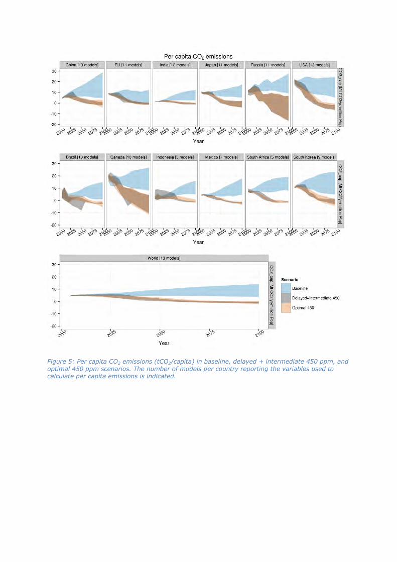
Figure 5: Per capita CO2 emissions (tCO2/capita) in baseline, delayed + intermediate 450 ppm, and
optimal 450 ppm scenarios. The number of models per country reporting the variables used to calculate per capita emissions is indicated.

Figure 6: Kyoto gas emissions (MtCO2e) in 2030 for Baseline, Delayed + intermediate 450, and
Optimal 450 scenarios. Filled bars show the median value across models, error bars show the 10th to 90th percentile range.
Emissions: CO2 Energy, CO2 Land Use, Non-CO2
Figure 7 shows the projected greenhouse gas emissions in 2050 in terms of CO2
emissions from fossil fuels and industry, CO2 emissions from land use, and non-
CO2 emissions. The emissions in each of these categories decline in the
mitigation scenarios with respect to the baseline projections, with land use
emissions even turning negative in some cases (Brazil, USA). CO2 emissions from
fossil fuels and industry represent the majority of global total emissions in the
baseline, while the mitigation scenarios result in about equal shares of non-CO2
emissions and CO2 emissions from fossil fuels and industry globally. There are,
however, regional differences. In China, for example, CO2 emissions from fossil
fuels and industry remain the major contributor to total emissions, while in
Indonesia, land use emissions represent the largest share.


Figure 7: CO2 emissions from energy supply and from land use, and non-CO2 emissions in 2050
(upper graph: MtCO2eq/year; lower graph: indexed to 2010) in baseline, delayed 450, intermediate 450 and optimal 450 scenarios.
Regional cumulative emissions
The scenarios can be used to calculate cumulative CO2 emissions over a given
period. These cumulative CO2 emissions can be interpreted as regional emission
constraints consistent with global climate policy targets assuming cost-efficient
implementation across the regions. Note that the cumulative emissions linked to
e.g. a <2°C temperature outcome need to be constantly updated to account for
revised estimates of past, current and future emissions as well as developments
in climate science. The regional cumulative emissions are presented in Figure 8
(median of all models). The difference in cumulative emissions between the

baseline and the mitigation scenarios is especially pronounced in China and
India.
Figure 8: Cumulative CO2 emissions (Gt CO2) between 2010 and 2100 per country / region and scenario, based on the median of the model ensemble. The number of models per country is indicated. The coloured areas are indicative of the emission reductions going from one scenario category to another. For instance, the black area indicates the additional emissions in the baseline
scenario compared to the current policy (reference) scenarios. The red area shows the additional emissions between current policies and 550 ppm CO2.
Peak Year
Figure 9 presents the peak year in CO2 emissions per region. Under the optimal
450 scenarios, most countries’ CO2 emissions peak before 2025 (except for
India, which peaks around 2030). Under delayed 450 scenarios, this peak
generally shifts to later in the century by construction, although not by much.
The peak year is even later in 500-550 ppm scenarios, especially in India and
Indonesia.

Comparison with the national model results
National scenarios for the European Union indicate that emissions have already
peaked, which is not the case for some of the global model scenario results. For
Brazil, the peak year of CO2 emissions in the reference scenario is projected to
be around 2060 (albeit with a large model spread), which is slightly later than
found by Herreras Martínez et al. (2015), whose reference scenario shows a peak
between 2045 and 2050. Peaking occurs considerably earlier in mitigation
scenarios for Brazil, around 2015 under delayed 450 scenarios. The 450 ppm
scenario by Herreras Martínez et al. (2015) peaks in 2020.
Figure 9: Peak year of CO2 emissions per country, in reference, 500-550 ppm, delayed 450 and optimal 450 scenarios. Models are plotted individually (coloured shapes), lines show the 5th, 50th and 95th percentiles of the range of model results.
Low-carbon energy technology as a function of cumulative
emissions
All countries show increasing deployment of low-carbon primary energy sources
with respect to carbon-intensive energy sources as stringency in mitigation
increases, i.e. lower cumulative emission scenarios, as shown in Figure 10. Low-
carbon primary energy sources are all primary energy sources except coal, gas
and oil without carbon capture and storage (CCS). For developed countries, this
generally means a substantial increase on 2010 levels. Some developing

countries, such as Brazil, India and Indonesia, on the other hand, show 2010
shares of low-carbon primary energy sources that are already close to the range
reached in mitigation scenarios (over 25% of total primary energy supply in
these cases).
Figure 11 shows that the share of low-carbon energy sources in electricity
generation increases substantially in mitigation scenarios, compared to baseline
scenarios. In 2030, the global average share of low-carbon energy sources is
roughly twice as high in mitigation scenarios as the share in baseline scenarios.

Comparison with the national model results
Mexico is projected to reach about a 65% – 100% share of low-carbon energy
sources in the mitigation scenarios, which is confirmed by Veysey et al. (2015).
They conclude that all models included in their study find a significant
decarbonisation necessary to reach Mexico’s greenhouse gas emission reduction
target, with ‘clean sources3’ reaching a share of 80% to 100% of electricity
generation by 2050.
The Brazilian national modelling team created their own intermediate 450
scenario for comparison, in which they defined low-carbon sources in the same
way as was used to produce Figure 11 (i.e. fossil fuels with CCS, nuclear,
biomass with and without CCS, and non-biomass renewables). They find high
shares of low-carbon sources in electricity generation, going from 79% in 2010
to 100% in 2050, mainly due to growth of non-biomass renewables (solar
photovoltaic, solar CSP, distributed solar, wind, wind offshore, hydropower and
ethanol). The global models project similar shares, reaching about 80%–100%
by 2050.
3 Defined as in Mexico’s Electricity Industry Law: non-biomass renewables, biomass, nuclear, and CCS technologies
(Veysey et al., 2015).

Figure 10: Share (%) of low-carbon primary energy sources (all sources except coal, gas and oil
without carbon capture and storage, CCS) in total primary energy supply in 2050, versus cumulative CO2 emissions (Gt CO2) between 2010 and 2100. The scenario categories are shown as colour. 2010 values are indicated by black dotted lines.

Figure 11: Share (%) of low-carbon energy sources in electricity generation (all sources except oil,
gas and oil without carbon capture and storage, CCS). The number of models per country is indicated.
Policy Costs
By 2030, the median policy costs under optimal 450 scenarios are higher than
those under delayed 450 scenarios for the world and for the region of China
(Figure 12). However, the delayed 450 scenarios result in higher policy costs by
2050, compared to the optimal 450 scenarios. This can be explained by the
steeper emission reductions needed in the longer term in the delayed 450
scenarios To some extent, these policy costs may be compensated by avoided
impacts of climate change, though economic modelling is beyond the scope of
this paper.

Note that the regions are covered by less models than for other variables shown
above, because models report different policy cost variables; here, consumption
loss is shown.
Figure 12: Policy costs (consumption loss), expressed as % of average costs in the 500-550 ppm scenarios of the same model, by 2030 and 2050, per country and scenario category. The number
of models per country reporting this cost variable is indicated. Categories include the reference scenario (current climate policies), the cost-optimal implementation of a 450 ppm target and the delayed implementation of a 450 ppm target (see methods).
How do assumptions on the availability of different technologies
influence these results?
Implications of Technology Availability Assumptions
The two modelling inter-comparison projects AMPERE and EMF27 have explored
the implications of different technology assumptions on scenario results. Figure

13 shows the different primary energy mixes for five different technology
assumptions as indicated in Table 5.
Table 5: Scenario categories used to evaluate technology availability implications (all scenario categories are variants of the AMPERE2-450-xxx-OPT scenario, thus assume an optimal 450 ppm pathway).
Scenario category Description
FullTech The default assumption of each model.
LowEI Assuming lower energy intensity of the economy, which can be interpreted as a higher efficiency of
end-use technologies, that are not explicitly represented in some of the models, or a less
materialistic evolution of the economy with a strong focus on the service sector, or a combination of both.
noCCS Assuming that carbon capture and storage will not be used (due to technology failures or as a political decision).
Conv A conventional world, with only limited biomass use (100 EJ globally is available) and the share of
variable power technologies (wind + solar) does not exceed 20% of electricity generation.
EERE A world of high efficiency and with focus on renewable energies. This combines the assumption of
LowEI and noCCS and additionally assumes a global phase-out of nuclear power after the end of the economic lifetime of all standing and currently
planned nuclear reactors.
For this analysis, we have selected the REMIND model for illustration, which
studied several variants of the AMPERE2-450-xxx-OPT scenario for the 6 regions
shown in Figure 13. REMIND was the only model able to provide all scenarios for
all 6 regions.
These different assumptions result in very strong differences in the deployment
of different technologies, with generally more deployment of the unrestricted
options, if one or several options are unavailable. Therefore, the extremes
observed in technology-restricted scenarios tend to be higher than in the default
scenario (FullTech). Moreover, the difference across scenarios is more important
than variability across regions. The results imply a large deployment of CCS for
India and Japan, which might raise feasibility problems. Furthermore, the high
use of biomass for some regions is improbable unless regions can import
biomass.

Figure 13: Primary energy mixes for 4 major economies + world under different assumptions on
technology availability in the REMIND model.
What are important co-benefits at the national/regional level of the
different policies?
Co-benefits
Energy Security and Energy Independence Co-benefits of Mitigation
Climate policies (both existing pledges4 (see e.g. Den Elzen et al., 2015,
Roelfsema et al., 2014) and 450 stabilization scenarios) globally lead to lower
energy trade (Cherp et al., 2013, Jewell et al., 2014, Jewell et al., 2013), but
both the uncertainty and the reduction in net-energy imports (or conversely
reduction in net-exports) from the baseline varies between countries and over
time. There are three types of national dynamics with respect to net-energy
trade. Firstly, energy importers generally experience a decrease in net-energy
imports in climate stabilization scenarios compared to the baseline development
while, secondly, energy exporters experience a loss of energy export revenues
from climate stabilization policies (Figure 14). However, the differences between
the baseline and the climate stabilization scenario are relatively small, except for
the Middle East and North Africa (MENA) region. The results for Canada are
influenced by one model showing a strong decrease in exports. Regional analyses
4 The Pledges scenario is the so-called “Stringent Policy” scenario from the LIMITS exercise (Kriegler et al., 2014b).

for Europe and the 2030 framework study show that energy imports decrease
with increasing ambition of climate policies, confirming the trends shown in
Figure 14.
Figure 14: Change in net-energy imports (left) and net-energy exports (right) for major energy importers and exporters. The number for each country represents the number of models. *Note: Reference Policy includes LIMITS-RefPol and AMPERE3-RefPol. Delayed-450 includes LIMITS-RefPol-450 and AMPERE3-450. Models include IMAGE, MESSAGE, REMIND, TIAM-ECN, WITCH, DNE and POLES. For China and India, we excluded one model which diverges from the trend of all the other models. In both cases, all but one model depict them as energy importers.
Thirdly, there are countries that in the baseline experience changes in their net-
energy trade (Table 6). For these countries, climate policies would likely not have
the biggest impact on their net-energy trade in the short term, but rather the
relative cost of extraction technologies and resource base development between
different regions. This dynamic is most pronounced in the USA, which becomes a
net energy exporter (primarily of coal) in most models between 2025 and 2060;
climate stabilization does not reverse this trend but delays it and prevents the
USA from developing significant energy export revenues in the latter half of the
century. For Mexico, as the country’s oil reserves are depleted, the country
becomes a net energy importer around 2030, followed by growing energy

imports. Climate stabilization curbs the growth of energy imports. Finally, Brazil
is characterized by very low energy imports today, which grow but plateau
around 2030 before becoming a net energy exporter around 2050.

Table 6: Countries with shifting net-energy dependence in the Baseline
Baseline Reference Policy Delayed-450
USA Becomes a net energy
exporter in most models (5
out of 7) between 2025 and
2060.
Similar to Baseline
but the shift is
delayed and coal
exports are lower.
Similar to
Baseline but loses
most energy
exports post
2050.
Mexic
o
Oil reserves are depleted,
and becomes energy
importer ~2030 followed by
growing imports.
Similar to Baseline Similar to
Baseline but lower
imports.
Brazil Very low energy imports
today. In Baseline, modest
growth in energy imports
which plateau ~2030.
Similar to Baseline Similar to
Baseline
Air Pollution Co-benefits of Mitigation
Achieving a 450 ppm stabilization scenario implies a fundamental transformation
of the global energy system. Such a transformation will not only result in the
required greenhouse gas emissions reductions, but will also affect the abundance
of air pollutants in the atmosphere. Greenhouse gas emissions, in particular CO2,
are reduced to a large degree by phasing out unabated fossil-fuel energy
production, like coal, and replacing them with less carbon intensive alternatives
like renewables or biomass energy. Because air pollutants are co-emitted with
CO2 during the combustion processes, changes in the energy system can result
in less or more air pollutants emissions.
Figure 15 shows that, across the board, sulphur dioxide emissions are strongly
reduced as a positive side-effect of greenhouse gas emission mitigation. This is
the case for both developing and developed countries. The main reason for this
reduction is that unabated coal combustion is a dominant source of sulphur
dioxide emissions, and this source of energy production needs to be rapidly
replaced by less carbon-intensive alternatives in order to achieve a 450
stabilization scenario.
Significant reductions can also be found for emissions of black carbon (soot).
However, because black carbon can be emitted during the combustion of fossil

fuels as well as from much less carbon-intensive energy sources, like biomass
(Bond et al., 2013), the effect can vary regionally. While, generally, black carbon
emissions are reduced together with emissions of greenhouse gases in 450
scenarios, some estimates show increasing black carbon emissions in countries
that strongly rely on bioenergy to achieve their greenhouse gas targets. In the
latter cases, more complementary policies are required to specifically reduce air
pollution from black carbon.
Figure 15: Changes in black carbon (brown) and sulphur dioxide (orange) emissions when moving from a baseline in absence of targeted new climate policies to a pathway in line with stabilizing
atmospheric CO2-equivalent concentrations at 450 ppm. Data is provided for 2030 (top) and 2050 (bottom). Dots show single model results, bars the full range. *Note: The LIMITS-Base (LIMITS1) scenario is taken as the baseline scenarios. LIMITS-RefPol-450 (LIMITS6) is taken as the 450 scenario. Models include IMAGE, MESSAGE, REMIND, GCAM, AIM, and WITCH. In case models did not report data at the national level, the reductions in air pollutants from the encompassing region were downscaled based on the shares found in the IMAGE model. Both the baseline and the 450 scenario assume a successful implementation of current air pollution legislation policies (CLE).

Conclusions
In this paper, we have looked into the regional results of a set of global models
in order to derive policy-relevant indicators at the national level and to compare
the insights of the global models with insights of national modelling teams.
General conclusions
The mitigation scenarios require major emission reductions in all
countries. These can only be achieved by a considerable change in
the energy supply of these countries. Primary energy demand
decreases strongly in the mitigation scenarios, compared to the baseline
scenario, especially in developing countries. The 450 scenarios show a
reduction in all countries of roughly 30-40% compared to the baseline.
There are regional differences, with e.g. South Africa showing a stronger
reduction in primary energy demand under mitigation scenarios.
Per capita CO2 emissions are projected to decline in all countries
under mitigation scenarios. Global average CO2 emissions reach
about 0.3 – 2 tCO2/capita under delayed 450 scenarios. Total CO2
emissions decrease in most countries under the mitigation scenarios, and
even turn negative in Brazil (due to land use, acting as a sink). In terms of
per capita emissions, developing countries generally remain below the
global average, although the upper end of the ranges for China, Indonesia
and South Africa are slightly above the global average. Most OECD
countries show per capita emissions ranges similar to or higher than the
global average. CO2 emissions from fossil fuels and industry represent the
majority of global total emissions in the baseline, while the mitigation
scenarios result in about equal shares of non-CO2 emissions and CO2
emissions from fossil fuels and industry globally. There are, however,
regional differences in the mitigation scenarios. In China, for example, CO2
emissions from fossil fuels and industry remain the major contributor to
total emissions, while in Indonesia, land use emissions represent the lion’s
share. The difference in cumulative emissions between the baseline and
the mitigation scenarios is especially pronounced in China and India
(assuming cost-efficient implementation across regions).
Under the optimal 450 scenarios, most countries’ CO2 emissions
peak before 2025 (except for India) and a phase-out of CO2
emission occurs around 2060. Under delayed and intermediate 450
scenarios (taking into account 2020 pledges and introducing optimal
policies between 2020 and 2025), this peak generally shifts to later in the
century, although not by much. The peak year is even later in 500-550
ppm scenarios, especially in India and Indonesia.
All countries show increasing shares of low-carbon primary energy
sources with lower cumulative emissions. For developed countries,
this generally means a substantial increase on 2010 levels. Some

developing countries, such as Brazil, India and Indonesia, on the other
hand, show 2010 shares of low-carbon primary energy sources that are
already close to the range reached in mitigation scenarios (over 25% of
total primary energy supply in these cases).
There is a cost advantage to starting mitigation early. Delayed 450
scenarios show lower median policy costs in the short term in some
regions (China and the world), but higher policy costs in the long term in
all regions, compared to the optimal 450 scenarios.
Comparison with national projections
In general the projections seem to be in line with those used at the
national level, although the latter show somewhat higher growth
rates in Brazil and India.
Primary energy intensity decreases strongly in all countries and all
scenarios, including the baseline scenario, but especially in developing
countries and the Russian Federation.
Co-benefits
Energy importing countries generally experience a decrease in net-
energy imports in climate stabilization scenarios compared to the
baseline development, while energy exporters experience a loss of
energy export revenues from climate stabilization policies.
Countries that experience changes in net energy trade in the baseline,
most notably the USA, are likely more affected by relative costs of
extraction technologies and resource base developments than by climate
policies.
Across the board, sulphur dioxide emissions are strongly reduced
as a positive side-effect of greenhouse gas emission mitigation.
This is the case for both developing and developed countries. Significant
reductions of black carbon emissions can also be found, albeit with
regional differences. Countries that strongly rely on bioenergy to reach
mitigation targets, for example, see increasing black carbon emissions,
thus requiring additional policies to reduce air pollution from black carbon.

Acknowledgements
This publication has been prepared by PBL and FEEM/CMCC for the MILES project
Consortium under contract to DG CLIMA (No.
21.0104/2014/684427/SER/CLIMA.A.4).
The MILES project
The MILES project (Modelling and Informing Low Emission Strategies) is an
international cooperation project between 19 research teams from emerging
countries like China, India and Brazil and research teams in developed countries
from Europe, the US and Japan. Key objectives of the project are: 1) to explore
different country-level strategies consistent with the 2oC target, 2) to increase
understanding of differences between strategies in different parts of the world,
and 3) to enhance in all participating countries the capacity to perform analysis
of mitigation strategies. This is implemented by sharing experience on i) scenario
definition to ensure the necessary level of detail in the definition of the low-
carbon strategies for informing national and international policy discussions on
decarbonisation, ii) model development to ensure the improvement of national
modelling capacities permitting the elaboration of modelling frameworks able to
represent a broad coverage of sectors, activities and GHG, and enable the
representation of socio-economic implications of policy choices; iii) comparative
and diagnostic model analysis to better understand the influence of model
structure on model results and iv) policy analysis of model results to identify
those trajectories that are relevant for the purpose of defining strategies and
policies that are both consistent with climate and development objectives.
This project is funded by the European Union.
Disclaimer: This publication was written by a group of independent experts who
have not been nominated by their governments. The contents of this publication
are the sole responsibility of PBL and FEEM/CMCC and can in no way be taken to
reflect the views of the European Union or any government, organization, etc.

References
BOND, T. C., DOHERTY, S. J., FAHEY, D. W., FORSTER, P. M., BERNTSEN, T., DEANGELO, B. J.,
FLANNER, M. G., GHAN, S., KÄRCHER, B., KOCH, D., KINNE, S., KONDO, Y., QUINN, P. K.,
SAROFIM, M. C., SCHULTZ, M. G., SCHULZ, M., VENKATARAMAN, C., ZHANG, H., ZHANG,
S., BELLOUIN, N., GUTTIKUNDA, S. K., HOPKE, P. K., JACOBSON, M. Z., KAISER, J. W.,
KLIMONT, Z., LOHMANN, U., SCHWARZ, J. P., SHINDELL, D., STORELVMO, T., WARREN, S.
G. & ZENDER, C. S. 2013. Bounding the role of black carbon in the climate system: A
scientific assessment. Journal of Geophysical Research: Atmospheres, 118, 5380-5552.
CHERP, A., JEWELL, J., VINICHENKO, V., BAUER, N. & DE CIAN, E. 2013. Global energy security
under different climate policies, GDP growth rates and fossil resource availabilities. Climatic
Change, 1-12.
CLARKE, L., JIANG, K., AKIMOTO, K., BABIKER, M., BLANFORD, G., FISHER VANDEN, K.,
HOURCADE, J., KREY, V., KRIEGLER, E., LÖSCHEL, A., MCCOLLUM, D., PALTSEV, S., ROSE,
S., R. SHUKLA, P., TAVONI, M., VAN DER ZWAAN, B. & VAN VUUREN, D. P. 2014.
Assessing Transformation Pathways. In: EDENHOFER, O., PICHS-MADRUGA, R., SOKONA,
Y., FARAHANI, E., KADNER, S., SEYBOTH, K., ADLER, A., BAUM, I., BRUNNER, S.,
EICKEMEIER, P., KRIEMANN, B., SAVOLAINEN, J., SCHLÖMER, S., VON STECHOW, C.,
ZWICKEL, T. & MINX, J. C. (eds.) Climate Change 2014: Mitigation of Climate Change.
Contribution of Working Group III to the Fifth Assessment Report of the Intergovernmental
Panel on Climate Change Cambridge, United Kingdom: Cambridge University Press.
DEN ELZEN, M. G. J., FEKETE, H., ADMIRAAL, A., FORSELL, N., HÖHNE, N., KOROSUO, A.,
ROELFSEMA, M., VAN SOEST, H., WOUTERS, K., DAY, T., HAGEMANN, M., HOF, A. &
MOSNIER, A. 2015. Enhanced Policy Scenarios for Major Emitting Countries. Analysis of
Current and Planned Climate Policies, and Selected Enhanced Mitigation Measures. The
Hague: PBL Netherlands Environmental Assessment Agency.
HERRERAS MARTÍNEZ, S., KOBERLE, A., ROCHEDO, P., SCHAEFFER, R., LUCENA, A., SZKLO, A.,
ASHINA, S. & VAN VUUREN, D. P. 2015. Possible energy futures for Brazil and Latin
America in conservative and stringent mitigation pathways up to 2050. Technological
Forecasting and Social Change.
JEWELL, J., CHERP, A. & RIAHI, K. 2014. Energy security under de-carbonization scenarios: An
assessment framework and evaluation under different technology and policy choices.
Energy Policy, 65, 743-760.
JEWELL, J., CHERP, A., VINICHENKO, V., BAUER, N., KOBER, T., MCCOLLUM, D., VAN VUUREN, D.
P. & VAN DER ZWAAN, B. 2013. Energy security of China, India, the E.U. and the U.S.
under long-term scenarios: Results from six IAMs. Climate Change Economics, 04,
1340011.
KRIEGLER, E., RIAHI, K., BAUER, N., SCHWANITZ, V. J., PETERMANN, N., BOSETTI, V., MARCUCCI,
A., OTTO, S., PAROUSSOS, L., RAO, S., ARROYO CURRÁS, T., ASHINA, S., BOLLEN, J.,
EOM, J., HAMDI-CHERIF, M., LONGDEN, T., KITOUS, A., MÉJEAN, A., SANO, F.,
SCHAEFFER, M., WADA, K., CAPROS, P., P. VAN VUUREN, D. & EDENHOFER, O. 2014a.
Making or breaking climate targets: The AMPERE study on staged accession scenarios for
climate policy. Technological Forecasting and Social Change.
KRIEGLER, E., TAVONI, M., ABOUMAHBOUB, T., LUDERER, G., CALVIN, K., DE MAERE, G., KREY,
V., RIAHI, K., ROSLER, H., SCHAEFFER, M. & VAN VUUREN, D. 2014b. What does the 2°C
target imply for a global climate agreement in 2020? The LIMITS study on Durban Platform
scenarios. Climate Change Economics, 4.
KRIEGLER, E., WEYANT, J. P., BLANFORD, G. J., KREY, V., CLARKE, L., EDMONDS, J., FAWCETT,
A., LUDERER, G., RIAHI, K., RICHELS, R., ROSE, S. K., TAVONI, M. & VAN VUUREN, D. P.

2014c. The role of technology for achieving climate policy objectives: Overview of the EMF
27 study on global technology and climate policy strategies. Climatic Change, 123, 353-
367.
RIAHI, K., KRIEGLER, E., JOHNSON, N., BERTRAM, C., DEN ELZEN, M., EOM, J., SCHAEFFER, M.,
EDMONDS, J., ISAAC, M., KREY, V., LONGDEN, T., LUDERER, G., MÉJEAN, A., MCCOLLUM,
D. L., MIMA, S., TURTON, H., VAN VUUREN, D. P., WADA, K., BOSETTI, V., CAPROS, P.,
CRIQUI, P., HAMDI-CHERIF, M., KAINUMA, M. & EDENHOFER, O. 2014. Locked into
Copenhagen pledges - Implications of short-term emission targets for the cost and
feasibility of long-term climate goals. Technological Forecasting and Social Change.
ROELFSEMA, M., DEN ELZEN, M. G. J., HÖHNE, N., HOF, A. F., BRAUN, N., FEKETE, H.,
BRANDSMA, R., LARKIN, J. & BÖTTCHER, H. 2014. Are major economies on track to
achieve their pledges for 2020? An assessment of domestic climate and energy policies.
Energy Policy.
TAVONI, M., KRIEGLER, E., RIAHI , K., VAN VUUREN, D. P., ABOUMAHBOUB, T., BOWEN, A.,
CALVIN, K., KOBER, T., JEWELL, J., LUDERER, G., MARANGONI, G., MCCOLLUM, D., VAN
SLUISVELD, M., ZIMMER, A. & VAN DER ZWAAN, B. 2014. Post-2020 climate agreements
in the major economies assessed in the light of global models. Nature Clim. Change,
Published on-lie.
UNFCCC 2010. Report of the Conference of the Parties on its sixteenth session, held in Cancun
from 29 November to 10 December 2010. Addendum. Part Two: Action taken by the
Conference of the Parties at its sixteenth session. Decision 1/CP.16: The Cancun
Agreements: Outcome of the work of the Ad Hoc Working Group on Long-term Cooperative
Action under the Convention. FCCC/CP/2010/7/Add.1.
VAN SLUISVELD, M. A. E., GERNAAT, D. E. H. J., ASHINA, S., CALVIN, K. V., GARG, A., ISAAC, M.,
LUCAS, P. L., MOURATIADOU, I., OTTO, S. A. C., RAO, S., SHUKLA, P. R., VAN VLIET, J. &
VAN VUUREN, D. P. 2013. A multi-model analysis of post-2020 mitigation efforts of five
major economies. Climate Change Economics, 04, 1340012.
VEYSEY, J., OCTAVIANO, C., CALVIN, K., MARTINEZ, S. H., KITOUS, A., MCFARLAND, J. & VAN
DER ZWAAN, B. 2015. Pathways to Mexico’s climate change mitigation targets: A multi-
model analysis. Energy Economics.


č


