1

Performance Evaluation of Computer Networks

Objectives Introduction to Queuing Theory Little’s Theorem Standard Notation of Queuing Systems Poisson Process and its Properties M/M/1 , M/M/m , M/M/m/m , and M/G/1

Queuing System Network of queues

Jackson Networks

2

Introduction Each one of us has spent a great deal of

time waiting in lines. One example in the Cafeteria Other examples of queues are

Printer queue Packets arriving to a buffer Calls waiting for answer by a technical support

3

What makes up a queue?

The System: A collection of objects under study It is important to define the system

boundariesThe Entities: The people, packets, or

objects that enter the system requiring some kind of service

The Servers: The people, resources, or servers that perform the service required

The Queue: An accumulation of entities that have entered the system but have not been served

4

Queue Discipline

First Come First Served - FCFS Most customer queues

Last Come First Served - LCFS Packages, Elevator

Served in Random Order - SIRO Entering Buses

Priority Service Multi-processing on a computer Emergency room

5

What factors effect system performance The Arrivals Process

The time between any two successive arrivals Does this depend on the number of packets in the system? Finite populations

The Service Process The time taken to perform the service Does this depend on the number of packets in the system?

The number of servers operating in system The Service Discipline System Capacity

Processes waiting + processes being served

6

Measuring System Performance The total time an “entity” spends in the

system (Denoted by W) The time an “entity spends in the queue

(Denoted by Wq) The number of “entities” in the system

(Denoted by L) The number of “entities” in the queue

(Denoted by Lq) The percentage of time the servers are busy

(Utilization time)

These quantities are variable over time

7

What is Queuing Theory?

Primary methodological framework for analyzing network delay

Often requires simplifying assumptions since realistic assumptions make meaningful analysis extremely difficult

Provide a basis for adequate delay approximation

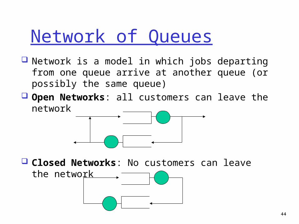
queue

8

Packet Delay

Packet delay is the sum of delays on each subnet link traversed by the packet

Link delay consists of: Processing delay Queuing delay Transmission delay Propagation delay

node

node

node

packet delay

link delay

9

Link Delay Components (1)

Processing delay Delay between the time the packet is

correctly received at the head node of the link and the time the packet is assigned to an outgoing link queue for transmission

head node tail node

outgoing link queue

processing delay

10

Link Delay Components (2)

Queuing delay Delay between the time the packet is

assigned to a queue for transmission and the time it starts being transmitted

head node tail node

outgoing link queue

queuing delay

11

Link Delay Components (3)

Transmission delay Delay between the times that the first and

last bits of the packet are transmitted

head node tail node

outgoing link queue

transmission delay

12

Link Delay Components (4)

Propagation delay Delay between the time the last bit is

transmitted at the head node of the link and the time the last bit is received at the tail node

head node tail node

outgoing link queue

propagation delay

13

Queuing System (1)

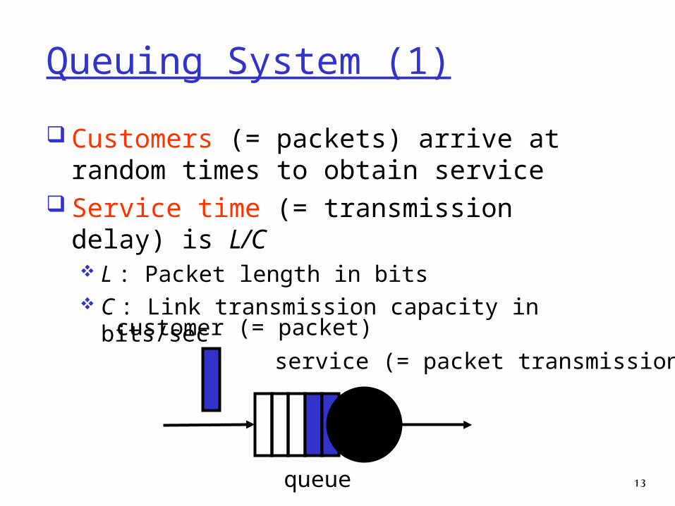
Customers (= packets) arrive at random times to obtain service

Service time (= transmission delay) is L/C L : Packet length in bits C : Link transmission capacity in bits/sec

queue

customer (= packet)

service (= packet transmission)

14

Queuing System (2)

Assume that we already know: Customer arrival rate Customer service rate

We want to know: Average number of customers in the system Average delay per customer

customer arrival rate

customer service rate

average delay

average # of customers

15

Little’s Theorem

16

Definition of Symbols (1)

pn = Steady-state probability of having n customers in the system

= Arrival rate (inverse of average interarrival time)

= Service rate (inverse of average service time)

N = Average number of customers in the system

17

Definition of Symbols (2)

NQ = Average number of customers waiting in queue

T = Average customer time in the system

WQ = Average customer waiting time in queue (does not include service time)

18

Little’s Theorem

N = Average number of customers = Arrival rate T = Average customer time in the

systemN = T

Hold for almost every queuing system that reaches a steady-state

Express the natural idea that crowded systems ( large N ) are associated with long customer delays ( large T ) and reversely

19

Application of Little’s Theorem (2) Consider a window flow control system

W : Window size : Packet arrival rate T : Average packet delay

From Little’s TheoremW >= T

If T increases, must eventually decrease If is limited due to congestion, increasing

W merely serves to increase T

20

Standard Notation of Queuing Systems

21

Standard Notation of Queuing Systems (1)

X/Y/Z/K X indicates the nature of the arrival process

M : Memoryless (= Poisson process, exponentially distributed interarrival times)

G : General distribution of interarrival times D : Deterministic interarrival times

Y indicates the probability distribution of the service times M : Exponential distribution of service times G : General distribution of service times D : Deterministic distribution of service times

22

Standard Notation of Queuing Systems (2)

X/Y/Z/K Z indicates the number of servers K (optional) indicates the limit on the

number of customers in the system Examples:

M/M/1, M/M/m, M/M/∞, M/M/m/m M/G/1, G/G/1 M/D/1, M/D/1/m

23

Poisson Process and its Properties

24

The Poisson Arrival Model

A Poisson process is a sequence of events “randomly spaced in time”

Examples Customers arriving to a bank Packets arriving to a buffer

The rate λ of a Poisson process is the average number of events per unit time (over a long time)

25

Properties of Poisson Process (1)

Interarrival times n are independent and exponentially distributed with parameter

The mean and variance of interarrival times n are 1/ and 1/^2, respectively

26

Properties of Poisson Process (2)

If two or more independent Poisson process A1, ..., Ak are merged into a single process A = A1 + A2 + ... + Ak, the process A is Poisson with a rate equal to the sum of the rates of its components

A1

Ai

Ak

A

independent Poisson processes

Poisson process

merge1

i

k

k

ii

1

27

Properties of Poisson Process (3)

If a Poisson process A is split into two other processes A1 and A2 by randomly assigning each arrival to A1 or A2, processes A1 and A2 are Poisson

A1

A2

A

Poisson processes

Poisson process

split randomly1

2

with probability p

with probability (1-p)

28

M/M/1 Queuing System

29

M/M/1 Queuing System

A single queue with a single server Customers arrive according to a Poisson

process with rate The probability distribution of the

service time is exponential with mean 1/

Poisson arrival with arrival rate

Exponentially distributed service timewith service rate

single server

infinite buffer

30

M/M/1 Queuing System: Results (1) Utilization factor (proportion of time the

server is busy)

Probability of n customers in the system

Average number of customers in the system

(1 )nnp

1N

31

M/M/1 Queuing System: Results (2) Average customer time in the system

Average number of customers in queue

Average waiting time in queue

1NT

2

1QN W

1W T

32

M/M/m Queuing System

33

M/M/m Queuing System

A single queue with m servers Customers arrive according to a Poisson

process with rate The probability distribution of the

service time is exponential with mean 1/

Poisson arrival with arrival rate Exponentially

distributedservice time with rate

m servers

infinite buffer

1

m

34

M/M/m Queuing System: Results (1) Ratio of arrival rate to maximal system

service rate

Probability of n customers in the system

m

10

0

0

0

1( ) ( )

! !(1 )

( )

!

!

m

k

n

nm m

k mm mp

k m

mp n m

npm

p n mm

35

M/M/m Queuing System: Results (2) Probability that an arriving customer

has to wait in queue (m customers or more in the system)

Average waiting time in queue of a customer

Average number of customers in queue

0( )

!(1 )

m

Qp m

Pm

(1 )

Q QN PW

0 1

QQ m n

n

PN np

36

M/M/m Queuing System: Results (3) Average customer time in the system

Average number of customers in the system

1 1 QPT W

m

1

QPN T m

37

M/M/m/m Queuing System

38

M/M/m/m Queuing System A single queue with m servers (buffer size

m) Customers arrive according to a Poisson

process with rate The probability distribution of the service

time is exponential with mean 1/

Poisson arrival with arrival rate Exponentially

distributedservice time with rate

m servers

buffer size m

1

m

39

M/M/m/m Queuing System: Results Probability of m customers in the

system

Probability that an arriving customer is lost

00

0

11

!

1, 1,2, ,

!

nm

n

n

n

pn

p p n mn

0

( / ) / !

( / ) / !

m

m m n

n

mp

n

40

M/G/1 Queuing System

41

M/G/1 Queuing System

A single queue with a single server Customers arrive according to a Poisson

process with rate The mean and second moment of the

service time are 1/and X2

Poisson arrival with arrival rate

Generally distributed service timewith service rate

single server

infinite buffer

42

M/G/1 Queuing System: Results (1) Utilization factor

Mean residual service time

2

2

XR

43

M/G/1 Queuing System: Results Pollaczek-Khinchin formula

2

1 2(1 )

1

R XW

T W

22

22

2(1 )

2(1 )

QX

N W

XN T

44

Network of Queues Network is a model in which jobs departing

from one queue arrive at another queue (or possibly the same queue)

Open Networks: all customers can leave the network

Closed Networks: No customers can leave the network

45

Jackson Networks

Jackson Network is named after James R. Jackson

It is the first significant development in the theory of networks of queues

Each node of the queueing network can be analyzed separately

The utilization of all of the queues is less than one

46

Open Jackson Networks

There are J queues Customers arrive at queue l according to independent

Poisson processes with rate The service times in queue l are exponential with rates Upon leaving queue l, each customer is sent to queue m with

probability and leaves the network with probability

The routing decision is independent of the past evolution of the network

l

l

lmr

J

mlmr

1

1

47

An Open Jackson Network

ii

j

k

k

j

ikrkjr

ijr

m

imr

48

Conclusion

Queuing models provide qualitative insights on the performance of computer networks, and quantitative predictions of average packet delay

To obtain tractable queuing models for computer networks, it is frequently necessary to make simplifying assumptions

A more accurate alternative is simulation, which, however, can be slow, expensive, and lacking in insight