1

PROBABILITY MODELS FOR ECONOMIC DECISIONS

Chapter 1: Simulation and Conditional Probability

The difficulties of decision-making under uncertainty are familiar to everyone. We all

regularly have to make decisions where we lack important information about factors that could

significantly affect the outcomes of our decisions. Decision analysis is the study of general

techniques for quantitatively analyzing decisions under uncertainty. This book offers an

introduction to decision analysis, with an emphasis on showing how to make sophisticated

models of economic decisions that involve uncertainty.

The idea of quantitatively analyzing uncertainty may seem puzzling at first. How can we

analyze what we do not know? The answer is that we can describe our information and

uncertainty in the language of probability theory, which is the basic mathematics of uncertainty.

Whenever there is something that we do not know, our uncertainty about it can (in principle) be

described quantitatively by probabilities. This book includes an introduction to the basic ideas of

probability theory, but the aim throughout is to show how probability theory can be applied to

gain understanding and insights into practical decision problems.

In recent decades, economists have increasingly recognized the critical impact of

uncertainty on decision-making, in the formulation of competitive strategies and financial plans.

So a professional economist has good reason to believe that the study of probability theory

should be an important technical topic in the training of business students. But in traditional

approaches to teaching probability, most business students see little or no connection between

probability theory and the practical decisions under uncertainty that they will confront in their

managerial careers. This disconnection occurs because the formulas which are traditionally

taught in basic probability courses become hard to apply in problems that involve more than one

or two unknown quantities, but realistic decision problems typically involve many unknown

quantities.

Recent advances in computer technology, however, allows us to teach probability

differently today, in ways that can eliminate this disconnection between theory and application.

Electronic spreadsheets, which were invented in the late 1970s, offer an intuitive graphical

2

display in which it much easier to visualize and understand mathematical models, even when

they involve large numbers of variables. Randomized ("Monte Carlo") simulation methods offer

a general way to compute probabilities without learning a lot of specialized formulas.

Mathematicians used to object that such simulation methods were computationally slow and

inefficient, but the increasing speed of personal computers has continually diminished such

computational concerns. So the emphasis throughout this book is on formulating randomized

simulation models in spreadsheets. With this approach, even in the first chapter, we can analyze

a model that involves 21 random variables.

Chapter 1 is an introduction to working with probabilities in simulation models.

Fundamental ideas of conditional probability are developed here, in the context of simple

examples about learning from observations. With these examples, we show how probabilities

can be used to construct a simulation model, and then how such a model can be used to estimate

other probabilities.

1.0 Getting started with Simtools in Excel

All the work in this book is done in Microsoft Excel. Within Excel, there are many

different ways of telling the program to do any one task. Most commands can begin by selecting

one of the options on the menu bar at the top of the screen ("File Edit View Insert Format Tools

Data Window Help") and then selecting among the secondary options that appear under the menu

bar. Many common command sequences can also be entered by a short-cut keystroke (which is

indicated in the pop-down menus), or by clicking on a button in a toolbar that you can display on

the screen (try the View menu). But in this book, I will describe command descriptions as if you

always use the full command sequence from the top menu. There are many fine books on Excel

that you may consult for more background information about using Excel.

Unfortunately, Excel by itself is not quite enough to do probabilistic decision analysis at

the level of this book. To fill in its weak spots, Excel needs to be augmented by a decision-

analysis add-in. In this book, we will use an add-in for Excel called simtools.xla which is

available on an accompanying disk and on the Internet at

http://home.uchicago.edu/~rmyerson/addins.htm

3

Simtools.xla is comparable to a number of other commercially available add-ins for decision

analysis, such as @Risk (www.palisade.com), Crystal Ball (www.decisioneering.com), and

Insight.xla (www.analycorp.com).

When you copy or download simtools.xla, you should save it in your macro library folder

under the Microsoft Office folder on your computer's hard disk, which is often called

C:\Program Files\Microsoft Office\Office\Library

Then, in Excel, you can install Simtools by using the Tools:Add-Ins command sequence and then

selecting the "Simulation Tools" option that will appear in the dialogue box. Once installed,

"Simtools" should appear as an option directly in Excel's Tools menu.

(Also available with simtools.xla is another add-in formlist.xla, for auditing formulas in

spreadsheets. All spreadsheets in this book have lists of formulas that were produced with the

help of this Formlist add-in, and I would recommend downloading and installing it along with

Simtools.)

1.1. How to toss coins in a spreadsheet

When we study probability theory, we are studying uncertainty. To study uncertainty

with a spreadsheet, it is useful to create some uncertainty within the spreadsheet itself. Knowing

this, the designers of Excel gave us one simple but versatile way to create such uncertainty: the

RAND() function. I will now describe how to use this function to create a spreadsheet that

simulates tossing coins (a favorite first example of probability teachers).

With the cursor on cell A1 in the spreadsheet, let us type the formula

=RAND()

and then press the Enter key. A number between 0 and 1 is displayed in cell A1. Then (by

mouse or arrow keys) let us move the cursor to cell B1 and enter the formula

=IF(A1<0.5,"Heads","Tails")

(The initial equals sign [=] alerts Excel to the fact that what follows is to be interpreted as a

mathematical formula, not as a text label. The value of an IF function is its second parameter

when the first parameter is a true statement, but its value is the third parameter when the first

parameter is false.) Now Excel checks the numerical value of cell A1, and if A1 is less than 0.5

4

then Excel displays the text "Heads" in cell B1, but if A1 is greater than or equal to 0.5 then

Excel displays the text "Tails" in cell B1.

If you observed this construction carefully, you would have noticed that the number in

cell A1 changed when the formula was entered into cell B1. In fact, every time we enter

anything into spreadsheet, Excel recalculates the everything in the spreadsheet and it picks a new

value for our RAND() function. (I am assuming here that Excel's calculation option is set to

"Automatic" on your computer. If not, this setting can be changed under Excel's Tools:Options

menu.) We can also force such recalculation of the spreadsheet by pushing the "Recalc" button,

which is the [F9] key in Excel. If you have set up this spreadsheet as we described above, try

pressing [F9] a few times, and watch how the number in cell A1 and the text in cell B1 change

each time.

Now let us take hands away from the keyboard and ask the question: What will be the

next value to appear in cell A1 after the next time that the [F9] key is pressed? The answer is

that we do not know. The way that the Excel program determines the value of the RAND()

function each time is, and should remain, a mystery to us. (The parentheses at the end of the

function's name may be taken as a sign that the value depends on things that we cannot see.) My

vague understanding is that the program does some very complicated calculations, which may

depend in some way on the number of seconds past midnight on the computer's clock, but which

always generate a value between 0 and 1. I know nothing else specific about these calculations.

The only thing that you and I need to know about these RAND() calculations is that the value,

rounded to any number of decimal digits, is equally likely to be any number between 0 and 1.

That is, the first digit of the decimal expansion of this number is equally likely to be 0, 1, 2, 3, 4,

5, 6, 7, 8, or 9. Similarly, regardless of the first digit, the second decimal place is equally likely

to be any of these digits from 0 to 9, and so on. Thus, the value of RAND() is just as likely to be

between 0 and .1 as it is to be between .3 and .4. More generally, for any number v, w, x, and y

that are between 0 and 1, if v ! w = x ! y then the value of the RAND() expression is as likely

to be between w and v as it is to be between y and x. This information can be summarized by

saying that, from our point of view, RAND() is drawn from a Uniform probability distribution

over the interval from 0 to 1.

5

The cell B1 displays "Heads" if the value of A1 is between 0 and 0.5, whereas it displays

"Tails" if A1 is between 0.5 and 1. Because these two intervals have the same length (0.5!0 =

1!0.5), these two events are equally likely. That is, based on our current information, we should

think that, after we next press [F9], the next value of cell B1 is equally likely to be Heads or

Tails. So we have created a spreadsheet cell that behaves like a fair coin toss every time we press

[F9]. We have our first simulation model.

After pressing [F9] to relieve your curiosity, you should press it a few more times to

verify that, although it is impossible to predict whether Heads or Tails will occur next in cell B1,

they tend to happen about equally often when we recalculate many times. It would be easier to

appreciate this fact if we could see many of these simulated coin tosses at once. This is easy to

do by using the spreadsheet's Edit:Copy and Edit:Paste commands to make copies of our

formulas in the cells A1 and B1. So let us make copies of this range A1:B1 in all of the first 20

rows of the spreadsheet. (Any range in a spreadsheet can be denoted by listing its top-left and

bottom right cells, separated by a colon.)

To copy in Excel, we must first select the range that we want to copy. This can be done

by moving the cursor to cell A1 and then holding down the shift key while we move the cursor to

B1 with the right arrow key. (Pressing an arrow key while holding down the shift key selects a

rectangular range that has one corner at the cell where the cursor was when the shift key was first

depressed, and has its opposite corner at the current cell. The selected range will be highlighted

in the spreadsheet.) Then, having selected the range A1:B1 in the spreadsheet, open the Edit

menu and choose Copy. Faint dots around the A1:B1 range indicate that this range has been

copied to Excel's "clipboard" and is available to be pasted elsewhere. Next, select the range

A1:A20 in the spreadsheet, and then open the Edit menu again and choose Paste. Now the

spreadsheet should look something like Figure 1.1 below. (The descriptions that appear in the

lower right corner of Figure 1.1 are just text that I typed into cells E17:E20, with the help of the

add-in Formlist.xla, which is available along with Simtools.xla.)

In Figure 1.1, we have made twenty copies of the horizontal range A1:B1, putting the

left-hand side of each copy in one of the cells in the vertical range A1:A20. So each of these

twenty A-cells contains the RAND() function, but the values that are displayed in cells A1:A20

1234567891011121314151617181920

A B C D E F G0.765196 Tails0.223048 Heads0.941351 Tails0.129491 Heads0.688211 Tails0.93142 Tails0.747859 Tails0.166433 Heads0.316867 Heads0.834753 Tails0.45684 Heads0.43939 Heads0.737932 Tails0.331283 Heads0.500878 Tails0.898716 Tails0.202086 Heads FORMULAS FROM RANGE A1:D200.656246 Tails A1. =RAND()0.518526 Tails B1. =IF(A1<0.5,"Heads","Tails")0.835384 Tails A1:B1 copied to A1:B20

6

Figure 1.1. Simulation of coin tossing in a spreadsheet.

are different. The value of each RAND() is calculated independently of all the other RANDs in

the spreadsheet. The spreadsheet even calculates different RANDs within one cell

independently, and so a cell containing the formula =RAND()-RAND() could take any value

between !1 and +1.

The word "independently" is being used here in a specific technical sense that is very

important in probability theory. When we say that a collection of unknown quantities are

independent of each other, we mean that learning the values of some of these quantities would

not change our beliefs about the other unknown quantities in this collection. So when we say

that the RAND() in cell A20 is independent of the other RANDs in cells A1:A19, we mean that

knowing the values of cells A1:A19 tells us nothing at all about the value of cell A20. If you

covered up cell A20 but studied the values of cells A1:A19 very carefully, you should still think

that the value of cell A20 is drawn from a uniform distribution over the interval from 0 to 1 (and

7

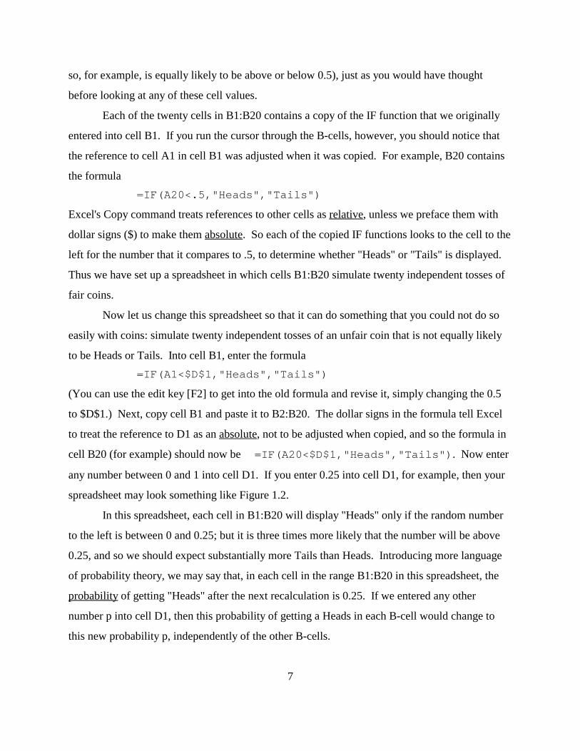
so, for example, is equally likely to be above or below 0.5), just as you would have thought

before looking at any of these cell values.

Each of the twenty cells in B1:B20 contains a copy of the IF function that we originally

entered into cell B1. If you run the cursor through the B-cells, however, you should notice that

the reference to cell A1 in cell B1 was adjusted when it was copied. For example, B20 contains

the formula

=IF(A20<.5,"Heads","Tails")

Excel's Copy command treats references to other cells as relative, unless we preface them with

dollar signs ($) to make them absolute. So each of the copied IF functions looks to the cell to the

left for the number that it compares to .5, to determine whether "Heads" or "Tails" is displayed.

Thus we have set up a spreadsheet in which cells B1:B20 simulate twenty independent tosses of

fair coins.

Now let us change this spreadsheet so that it can do something that you could not do so

easily with coins: simulate twenty independent tosses of an unfair coin that is not equally likely

to be Heads or Tails. Into cell B1, enter the formula

=IF(A1<$D$1,"Heads","Tails")

(You can use the edit key [F2] to get into the old formula and revise it, simply changing the 0.5

to $D$1.) Next, copy cell B1 and paste it to B2:B20. The dollar signs in the formula tell Excel

to treat the reference to D1 as an absolute, not to be adjusted when copied, and so the formula in

cell B20 (for example) should now be =IF(A20<$D$1,"Heads","Tails"). Now enter

any number between 0 and 1 into cell D1. If you enter 0.25 into cell D1, for example, then your

spreadsheet may look something like Figure 1.2.

In this spreadsheet, each cell in B1:B20 will display "Heads" only if the random number

to the left is between 0 and 0.25; but it is three times more likely that the number will be above

0.25, and so we should expect substantially more Tails than Heads. Introducing more language

of probability theory, we may say that, in each cell in the range B1:B20 in this spreadsheet, the

probability of getting "Heads" after the next recalculation is 0.25. If we entered any other

number p into cell D1, then this probability of getting a Heads in each B-cell would change to

this new probability p, independently of the other B-cells.

1234567891011121314151617181920

A B C D E F G0.129665 Heads 0.25 P(Heads) on each toss0.526313 Tails0.604349 Tails0.775623 Tails0.599284 Tails0.938539 Tails0.634633 Tails0.171716 Heads0.981668 Tails0.494835 Tails0.356306 Tails0.058359 Heads0.944084 Tails0.946007 Tails0.840926 Tails0.612527 Tails0.779595 Tails FORMULAS FROM RANGE A1:D200.219282 Heads A1. =RAND()0.4022 Tails B1. =IF(A1<$D$1,"Heads","Tails")

0.267915 Tails A1:B1 copied to A1:B20

8

Figure 1.2. Coin tossing with adjustable probabilities.

More generally, when I say that the probability of some event "A" is some number q

between 0 and 1, I mean that, given my current information, I think that this event "A" is just as

likely to occur as the event that any single RAND() in a spreadsheet will take a value less than q

after the next recalculation. That is, I would be indifferent between a lottery ticket that would pay

me $100 if the event "A" occurs and a lottery ticket that would pay me $100 if the RAND()'s next

value is less than the number q. When this is true, I may write the equation P(A) = q.

1.2. A simulation model of twenty sales calls

Perhaps it seems somewhat frivolous to model 20 coin tosses. So let us consider instead

a salesperson who will call on 20 customers this week. In each sales call, the salesperson may

make a sale or not. To adapt the spreadsheet in Figure 1.2 to this situation, let us begin by re-

editing the formula in cell B1 to simulate the first sales call. So instead of displaying "Heads" or

"Tails", the cell should display either 1, to represent a sale, or 0, to represent no-sale. The

9

RAND() value that determines the value of this cell can actually be generated inside the cell's

formula itself. So let us select cell B1 and change its formula to

=IF(RAND()<$D$1,1,0)

Next, copy this cell B1 and paste it to the range B1:B20, and you should see a column of random

0's and 1's in B1:B20, simulating the results of twenty sales calls.

We should have a label above this column of 0's and 1's to remind ourselves that they

represent sales. We also do not need the column of RANDs on the left any more. So let us first

eliminate the current leftmost column by selecting cell A1 and using the command sequence

Edit:Delete:EntireColumn. Next, let us insert a new top row by selecting (the new) A1 and using

the command sequence Insert:Rows. Notice that the cell that was originally B1 has now become

cell A2, and its formula is now

=IF(RAND()<$C$2,1,0)

(Excel has automatically adjusts all references appropriately when row or columns are inserted or

deleted in a spreadsheet. Dollar-signs make a reference "absolute" only for the process of

copying and pasting.)

Let us now enter the label 'Sales in the new empty cell A1. If we enter the value

0.5 into cell C2 then, with our new interpretation, this spreadsheet simulates a situation in which

the salesperson has a probability 1/2 of making a sale with each of his 20 customers. So we

should enter the label

'P(Sale) in each call

into cell C1.

Indicating sales and no-sales in the various calls by 1s and 0s makes it easy for us to

count the total number of sales in the spreadsheet. We can simply enter the formula

=SUM(A2:A21) into cell C8 (say), and enter the label 'Total Sales in 20 calls

into the cell above. The result should look similar to Figure 1.3.

123456789101112131415161718192021

A B C D ESales? P(Sale in each call)

1 0.500101 Total Sales in 20 calls1 81100000110 FORMULAS FROM RANGE A1:C210 A2. =IF(RAND()<$C$2,1,0)0 A2 copied to A2:A210 C8. =SUM(A2:A21)

10

Figure 1.3. Simple model of independent sales calls.

This Figure 1.3 simulates the situation for a salesperson whose selling skill is such that he

has a probability 0.50 of making a sale in any call to a customer like these twenty customers. A

more skilled salesperson might be more likely to make a sale in each call. To simulate 20 calls

by a more (or less) skilled salesperson, we could simply replace the 0.50 in cell D2 by a higher

(or lower) number that appropriately represents the probability that this salesperson will get a

sale from any such call, given his actual level of skill in selling this product. In this sense, we

may think of a salesperson's probability of making a sale in any call to a customer like these as

being a numerical measure of his "skill" at this kind of marketing.

But once the number 0.50 is entered into cell C2 in Figure 1.3, the outcomes of the 20

simulated sales calls are determined independently, because each depends on a different RAND

variable in the spreadsheet. In this spreadsheet, if we knew that the salesperson made sales to all

of the first 19 customers, we would still think that his probability of making a sale to the 20th

customer is 1/2 (as likely as a RAND() being less than 0.50). Such a strong independence

11

assumption may seem very unrealistic. In real life, even if we knew that this company's

salespeople generally make sales in about half of their calls, a string of 19 successful visits might

cause us to infer that this particular salesperson is very highly skilled, and so we might think that

he would be much more likely to get a sale on his 20th visit. On the other hand, if we learned

that this salesperson had a string of 19 unsuccessful calls, then we might infer that he was

probably unskilled, and so we might think him unlikely to make a sale on his twentieth call. To

take account of such dependencies, we need to revise our model to one in which the outcomes of

the 20 sales calls are not completely independent.

This independence problem is important to consider whenever we make simulation

models in spreadsheets. The RAND function makes it relatively easy for us to make many

random variables and events that are all independent of each other. Making random variables

that are not completely independent of each other is more difficult. In Excel, if we want the

random values of two cells to not be independent of each other, then there must be at least one

cell with a RAND function in it which directly or indirectly influences both of these cells. (You

can trace all the cells which directly and indirectly influence any selected cell by repeatedly using

the Tools:Auditing:TracePrecedents command sequence until it adds no more arrows. Then use

Tools:Auditing:RemoveAllArrows.) So to avoid assuming that the sales simulated in A2:A21

are completely independent, we should think about some unknown quantities or factors that

might influence all these sales events, and we should revise our spreadsheet to take account of

our uncertainty about such factors.

Notice that the our concern about assuming independence of the 20 sales calls was really

motivated in the previous discussion by our uncertainty about the salesperson's skill level. This

observation suggests that we should revise the model so that it includes some explicit

representation of our uncertainty about the salesperson's skill level. The way to represent our

uncertainty about the salesperson's skill level is to make the skill level in cell C2 into a random

variable. When C2 is random, then the spreadsheet will indeed have a random factor that

influences all the twenty sales events. Making C2 random is appropriate because we do not

actually know the salesperson's level of skill. As a general rule in our probability modeling,

whenever we have significant uncertainty about a quantity, it is appropriate to model this quantity

12

as a random variable in our spreadsheets.

To keep things as simple as possible in this introductory example, let us suppose (for

now) that the salesperson has just two possible skill levels: a high level of skills in which he has

a 2/3 probability of making a sale from any call, and a low level of skills in which he has a 1/3

probability of making a sale from any call. Under this assumption, we may simply say that the

salesperson is "skilled" if he has the high level of skills that give him a 2/3 probability of selling

in any sales call; and we may say that he is "unskilled" if he has the low level of skills that give

him a probability 1/3 of selling in any sales call. For simplicity, let us also suppose that, before

observing the outcomes of any sales calls, we think that this salesperson is equally likely to be

either skilled or unskilled in this sense. To model this situation, we can modify the simple model

in Figure 1.3 by entering the formula

=IF(RAND()<0.5,2/3,1/3)

into cell C2. Then we can enter the label 'Salesperson's level of Skill into

cell C1, and the result should be similar to Figure 1.4.

If we repeatedly press the Recalc key [F9] for the spreadsheet in Figure 1.4, we can see

the value of cell D2 changing between 0.666667 and 0.333333. When the value is 0.666667, the

spreadsheet model is simulating a skilled salesperson. When the value is 0.333333, the

spreadsheet model is simulating an unskilled salesperson. When the salesperson is skilled, he

usually succeeds in more than half of his sales opportunities; and when he is unskilled, he usually

fails in more than half of the calls. But if you recalculate this spreadsheet many times, you

should occasionally see it simulating a salesperson who is skilled but who nevertheless fails in

more than half of his twenty calls.

123456789101112131415161718192021

A B C D E F GSales? Salesperson's level of Skill

1 0.3333330 (potential rate of sales in the long run)1101 Total Sales in 20 calls0 910 The results of these 20 sales-calls are0 conditionally independent given the Skill.10 FORMULAS FROM RANGE A1:C210 C2. =IF(RAND()<0.5,2/3,1/3)1 A2. =IF(RAND()<$C$2,1,0)0 A2 copied to A2:A210 C8. =SUM(A2:A21)1010

13

Figure 1.4. Model of 20 sales calls with uncertainty about salesperson's skill.

Let us now ask a question that might arise in the work of a supervisor of such

salespeople. If the salesperson sold to exactly 9 of the 20 customers on whom he called this

week, then what should we think is the probability that he is actually skilled (but just had bad

luck this week)? Remember: we are assuming that we believed him equally likely to be skilled

or unskilled at the beginning of the week; but observing 9 sales in 20 gives us some information

that should cause our beliefs to change.

To answer this question with our simulation model, we should recalculate the simulation

many times. Then we can see how often do skilled salespeople make only 9 sales, and how often

do unskilled salespeople make 9 sales. The relative frequencies of these two events in many

recalculated simulations will give us a way to estimate how much can be inferred from the

evidence of only 9 sales.

There is a problem, however. Our model is two-dimensional (spanning many rows and

14

several columns), and it is not so easy to make hundreds of copies of it. In this simple example,

we could put the whole model into 22 cells of a single row of the spreadsheet, and then we could

make thousands of copies of the model in the rows of our spreadsheet, but recopying a random

model thousands of times would be make for slow calculations in the spreadsheet, and this

technique would become unwieldy in even a slightly more complicated model.

But we do not really need a spreadsheet to hold thousands of copies of our whole model.

In our simulation, we only care about two things: is the salesperson skilled; and how many sales

did he make? So if we ask Excel to recalculate our model many times, then we only need it to

make a table that records the answers to these two questions for each recalculated simulation.

All the other information (about which customers among the twenty in A2:A21 actually

bought) that is generated in the repeated recalculations of the model can be erased as the next

recalculation is done. Excel has the capability to make just such a table, which is called a "data

table" in the language of spreadsheets. Simtools gives us a special version of the data table,

called a "simulation table," which is particularly convenient for analyzing such models.

To make a simulation table with Simtools, the output from our model that we want to

store in the table must be listed together in a single row. This model-output row must also have

at least one blank cell to its left, and beneath the model-output row there must be many rows of

blank cells where the simulation data will be written. In our case, the simulation output that we

want is in cells C2 and C8, but we can easily repeat the information from these cells in an

appropriate model-output row. So to keep track of whether the simulated salesperson's skill is

high, let us enter the formula =IF(C2=2/3,1,0) into cell B35, and to keep track of the

number of sales achieved by this simulated salesperson, let us enter the formula =C8 into cell

C35. To remind ourselves of the interpretations of these cells, let us enter the labels 'Skill

hi? and '#Sales into cells B34 and C34 respectively. In cells B34 and B35 here, we apply

here the convention that, whenever a Yes/No question is posed in a spreadsheet, the value 1

denotes "Yes" and the value 0 denotes "No".

Now we select the range in which the simulation table will be generated. The top row of

the selected range must include the model-output range B35:C35 and one additional unused cell

to the left (cell A35). So we begin by selecting the cell A35 as the top-left cell of our simulation

3031323334

353637383940414243444546

A B CFORMULASB35. =IF(C2=2/3,1,0)C35. =C8

Skill hi? Sales

SimTable 0 50 0 5

0.001 0 90.002 0 40.003 0 60.004 1 160.005 1 120.006 0 60.007 0 60.008 0 30.009 0 70.01 0 9

15

Data continues to row 1036 Figure 1.5. Simulation table formodel of twenty sales calls.

table. With the [Shift] key held down, we can then press the right-arrow key twice, to select the

range A35:C35. Now, when we extend the selected range downwards, any lower row that we

include in the selection will be filled with simulation data. If we want to record the results of

about 1000 simulations, then we should include in our simulation table about 1000 rows below

A35:C35. So continuing to hold down the [Shift] key, we can press the [PgDn] key to expand

our selection downwards. Notice that the number of rows and columns in the range size is

indicated in the formula bar at the top left of the screen (or in a pop-up box near the bottom of

the selected range) while we are using the [PgDn] or arrow keys with the [Shift] key held down.

Let us expand the selection until the range A35:C1036 is selected, which gives us 1002 rows that

in our selected range: one row at the top for model output and 1001 rows underneath it in which

to store data. (We will see that SimTable output looks a bit nicer when the number of data rows

is 1 plus a multiple of 100.) Finally, with this range A35:C1036 selected, we enter the command

sequence Tools:Simtools:SimulationTable. After a pause for some computations, the result

should look similar to Figure 1.5 below.

16

The data from the 1001 simulations are stored in B36:C1036 as values that do not change

when we recalculate the spreadsheet by pressing [F9]. Having these values fixed will be

important, because it will allow us to sort the data and analyze it statistically without having it

change every time we calculate another statistic. But above the data range, the model-output

cells B35:C35 still contain the formulas that link them to our simulation model, and so these two

cells will change when [F9] is pressed.

In the cells A36:A1036, on the left edge of the simulation table, Simtools has entered

percent-rank values that show, for each row of simulation data, what fraction of the other data

rows are above this row. Because we selected a range with 1001 data rows, these percentile

numbers increase by 1/1000 per row, increasing from 0 in the first data row (row 36) to 1 in the

last data row (row 1036). (Using 1001 data rows gives us nice even 1/1000 increments here

because each data row has 1000 "other data rows" above and below it. These percentile-ranks

will be used later for making cumulative distribution charts, after sorting the simulation data.)

Now, recall our basic question: What we can infer about the salesperson's skill level if he

gets 9 sales in 20 calls? Paging down the data range, we may find some rows where a skilled

salesperson got 9 sales, but most of the cases where 9 sales occurred are cases where the

salesperson was unskilled. To get more precise information out of our huge data set, we need to

be able to efficiently count the number of times that 9 sales (or any other number of sales)

occurred with either skill level.

To analyze the skill levels where in the simulations where a salesperson made exactly 9

sales, let us first enter the number 9 into the cell E33. (Cell E33 will be our comparison cell that

we can change if we want to count the number of occurrences of some other number of sales.)

Next, into cell E36, enter the formula

=IF(C36=$E$33,B36,"..")

Then copy the cell E36 and paste it to the range E36:E1036. Now the cells in the E column

display the value 1 in each data row where a skilled salesperson gets 9 sales, the value 0 in each

data row where an unskilled salesperson gets 9 sales, and the label ".." in all other data rows.

(Notice the importance of having absolute references to cell $E$33 in the above formulas, so that

they do not change when they are copied.) With the cells in E36:E1036 acting as counters, we

17

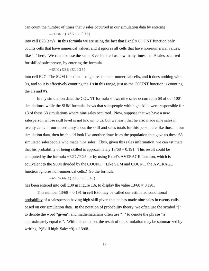
can count the number of times that 9 sales occurred in our simulation data by entering

=COUNT(E36:E1036)

into cell E28 (say). In this formula we are using the fact that Excel's COUNT function only

counts cells that have numerical values, and it ignores all cells that have non-numerical values,

like ".." here. We can also use the same E cells to tell us how many times that 9 sales occurred

for skilled salesperson, by entering the formula

=SUM(E36:E1036)

into cell E27. The SUM function also ignores the non-numerical cells, and it does nothing with

0's, and so it is effectively counting the 1's in this range, just as the COUNT function is counting

the 1's and 0's.

In my simulation data, the COUNT formula shows nine sales occurred in 68 of our 1001

simulations, while the SUM formula shows that salespeople with high skills were responsible for

13 of these 68 simulations where nine sales occurred. Now, suppose that we have a new

salesperson whose skill level is not known to us, but we learn that he also made nine sales in

twenty calls. If our uncertainty about the skill and sales totals for this person are like those in our

simulation data, then he should look like another draw from the population that gave us these 68

simulated salespeople who made nine sales. Thus, given this sales information, we can estimate

that his probability of being skilled is approximately 13/68 = 0.191. This result could be

computed by the formula =E27/E28, or by using Excel's AVERAGE function, which is

equivalent to the SUM divided by the COUNT. (Like SUM and COUNT, the AVERAGE

function ignores non-numerical cells.) So the formula

=AVERAGE(E36:E1036)

has been entered into cell E30 in Figure 1.6, to display the value 13/68 = 0.191.

This number 13/68 = 0.191 in cell E30 may be called our estimated conditional

probability of a salesperson having high skill given that he has made nine sales in twenty calls,

based on our simulation data. In the notation of probability theory, we often use the symbol "*"

to denote the word "given", and mathematicians often use "." to denote the phrase "is

approximately equal to". With this notation, the result of our simulation may be summarized by

writing P(Skill high*Sales=9) . 13/68.

232425262728293031323334

353637383940414243444546

A B C D E F GFORMULAS FROM RANGE A26:E1036B35. =IF(C2=2/3,1,0)C35. =C8 With Sales=9:E36. =IF(C36=$E$33,B36,"..") Frequency in Simtable:E36 copied to E36:E1036 13 Skill hiE27. =SUM(E36:E1036) 68 TotalE28. =COUNT(E36:E1036) P(Skill hi|Sales=9)E30. =AVERAGE(E36:E1036) 0.191176E25. ="With Sales="&E33&":"

Given Sales=9

Skill hi? Sales

SimTable 1 16 Skill hi?0 0 5 ..

0.001 0 9 00.002 0 4 ..0.003 0 6 ..0.004 1 16 ..0.005 1 12 ..0.006 0 6 ..0.007 0 6 ..0.008 0 3 ..0.009 0 7 ..0.01 0 9 0

18

Figure 1.6. Simulation data and analysis.

In a probability model like this one, where we learn about some unknown quantity by

observing other events that depend on it, the probabilities that describe our beliefs before the

observation are called prior probabilities, and the conditional probabilities that describe our

beliefs after the observation are called posterior probabilities. With this terminology, we could

say that, in this example, our prior probability of the salesperson's skill being high is 1/2, but our

posterior probability of his skill being high after we observe 9 sales in twenty calls should be

only about 0.2.

(Note: The labels in cells E25 and E29 in Figure 1.6 have been set up so that the number

"9" that is displayed will change when the value of cell E33 changes. Each of these cells actually

contains a formula that builds up the label using &, which is Excel's concatenation operator.

Thus, cell E29 actually contains the text formula

19

= "With Sales=" & E33 & ":"

returns the label "With Sales=9:" when cell E33 has the value 9. Similarly, the formula

= "P(Skill hi|Sales=" & E33 & ")"

returns the label "P(Skill hi|Sales=9)" in cell E29 in Figure 1.6 (even though this formula is not

actually listed in the figure). Throughout this book, our figures that show spreadsheets will list

all the formulas that are used in numerical computations, but we may omit some formulas that

are used for generating such live text labels.)

1.3. Analysis using Excel's Data-Table command

Changing the 9 in cell E33 to other numbers, we can see the outcome frequencies for

other sales numbers. But it would be helpful to make a table in which we can see together the

results for all sales numbers from 0 to 20. Such a table can be easily made with Excel's data-

table command (sometimes called a "what-if table" in other spreadsheet programs).

Here we will learn to use one form of data table called a column-input data table. The

structure of a column-input data table is similar to the simulation table that we made in the

previous section. (This similarity is not coincidental, because Simtools actually uses Excel's

column-input data tables to make its simulation tables.)

To make our data table, we must first make a row that contains the outputs from our

model that we want listed in the table, and there must be a blank range under this row where the

table will be made. In this case, we want to make a table of the recalculated values of the

frequency numbers and conditional probabilities listed in cells E27, E28, and E30 of Figure 1.6,

but there these are not in a row and there are not enough blank cells underneath these cells to

make the data table there. So let us enter the formula =E28 into cell I34, to echo there the

number of salespeople who made the given number of sales in cell E33. Next let us enter the

formula =E27 into cell J34, to display there the number of skilled people who made the given

number of sales. To compute the number of unskilled people who made the given number of

sales, let us enter the formula =I34-J34 into cell K34. To compute the fraction of skilled

salespeople among those who mader the given number of sales, let us enter the formula

=J34/(J34+K34) into cell L34. This range I34:L34 will be the output range at the top of the

262728293031323334

353637383940414243444546474849505152535455

H I J K L MFORMULAS FROM RANGE H34:L55I34. =E28J34. =E27K34. =I34-J34L34. =J34/(J34+K34)I35:L55. {=TABLE(,D34)}

Frequencies: Sales: Total Skill Hi Skill Lo P(Skill=Hi|Sales)(,E33) 68 13 55 0.1911765

0 0 0 0 #DIV/0!1 1 0 1 02 9 0 9 03 25 0 25 04 49 0 49 05 82 0 82 06 82 0 82 07 105 3 102 0.02857148 67 5 62 0.07462699 68 13 55 0.191176510 61 32 29 0.524590211 65 55 10 0.846153812 75 70 5 0.933333313 75 73 2 0.973333314 82 82 0 115 76 75 1 0.986842116 50 50 0 117 23 23 0 118 5 5 0 119 1 1 0 120 0 0 0 #DIV/0!

20

Figure 1.7. Data table of results for different numbers of sales.

data table. Underneath, the data table will list the recalculated the values of these cells as the

parameter in cell E33 is adjusted from 9 to other values between 0 and 20.

The other values that we want to substitute into cell E33 must be listed in the column to

the left of the output range, in the rows below it. So we must enter the numbers 0 to 20 into the

cells from H35 to H55. (To do so quickly, first enter the number 0 into cell H35, and then select

the range H35:H55 and use the command sequence Edit:Fill:Series with the Series dialogue-box

21

options: Columns, Linear, StepValue 1, and StopValue 20.)

Now we select the range H34:L55 and use the command sequence Data:Table. When the

"Row and Column Input" dialogue box comes up, we leave the "Row Input" entry blank, but we

tab to the "Column Input" box and enter cell E33 as the Column Input Cell.

Following this Data:Table command, Excel will compute the data entries into the range

I35:L55 as follows. For each row in this range, Excel first takes the value of the cell in column H

(the leftmost column in our selected range H34:L55) and enters it into cell E33. Then Excel

recalculates the whole spreadsheet. The new values of the output row at the top of the data table

I34:L34 are then copied down into the corresponding (I to L) cells in this row. When all the cells

in I35:K55 have been filled in this way, Excel restores the original contents of the input cell E33

(the value 9). Notice in Figure 1.7 that the data in row 44 of the data table (I44:K44) is identical

to the output above in I34:K34, because row 44 is based on the input value of 9 (from H44),

which is the actual current value of cell E33 (as shown previously in Figure 1.6).

If you check the formulas in the cells from I35 to L55, you will find that they all share the

special formula {=TABLE(,E33)}. The braces mean that this is an array formula, which

Excel has entered into the whole range I35:L55 at once. (Excel will not let you change any one

cell in an array; you have to change all or none. To emphasize that these cells together form an

array, I have put a border around the data range I35:L55 in Figure 1.7, using a Format:Cells

command.) The TABLE formula tells us that this range contains the data range of a data table

that has no row-input cell but has E33 as its column-input cell. But recall that the whole range

that we selected before invoking the Data:Table command also included one row above this data

range and one column to the left of this data range. The column on the left side of the data table

contains the alternative input values that are substituted one at a time into the designated column-

input cell. The row at the top of the data table contains the output values that were recalculated

and entered into the table below as as these alternative substitutions are done.

The conditional probability of any event A given some other event B, denoted by the

formula P(A*B), is the probability that we would assign to this event A if we learned that the

event B occurred. So the ratios in the L column of the data table give us estimates of the

conditional probability of a salesperson's having high skill, given the total number of sales that he

22

has made in twenty calls. Notice how these conditional probabilities of having high skill

increase from 0 to 1 as the given sales total increases. If the salesperson made only 7 sales in

twenty calls, then we would estimate that his conditional probability of being skilled was only

about 0.02. But if he made 12 sales out of twenty calls, then we would estimate that his

conditional probability of being skilled was about 0.93, according to the simulation data in this

spreadsheet.

Our simulation table gives us no data in Figure 1.7 for the extreme cases of 0 or 20 sales.

But it is obvious from the entries immediately below cell L35 that finding 0 successes in the 20

trials should make us almost sure that the salesperson is unskilled. Similarly, the entries just

above cell L55 indicate clearly that 20 successes out of 20 trials should make us almost sure that

the salesperson is skilled.

(Note: I can now tell you how you could make a simulation table if you did not have the

Simtools add-in for Excel. Recall that we prepared to make our simulation table by putting our

model output in cells B35 and C35, as shown in Figures 1.5 and 1.6. Then we selected a range

that had these cells B35:C35 plus the next cell on the left, A35, as its top row, and that also

included 1001 more rows below. With this range A35:C1036 selected, we used the command

sequence Tools:Simtools:SimulationTable. If you did not have Simtools then, after selecting the

range A35:C1036, you could instead use the command sequence Data:Table. When the dialogue

box asks you to specify input cells, leave the row-input box blank, and specify a column-input

cell that has no effect on any of our calculations, such as cell A34 or A35. The result will be that

Excel then recalculates the model 1001 times and stores the results in the rows of B36:C1036,

just as before. The column-input substitutions affect nothing, but the recalculation of the

RANDs gives us different results in each row. Unfortunately, Excel data tables are alive, in the

sense that they will be recalculated every time we recalculate the spreadsheet. When we do

statistical analysis, we will not want our simulation data to keep changing. To fix this, you could

select the data range B36:C1036, copy it to the clipboard by Edit:Copy, and then with

B36:C1036 still selected use the command sequence Edit:PasteSpecial:Values. The result is that

the TABLE formulas in the data range are replaced by the values that were displayed, and these

numerical values now will not change when [F9] is pressed. The Simtools simulation-table

0

20

40

60

80

100

120

0 1 2 3 4 5 6 7 8 9 10 11 12 13 14 15 16 17 18 19 20

Number of Sales

Freq

uenc

y in

Sim

ulat

ion

Skill Low

Total

Skill Hi

23

Figure 1.8. Frequencies of sales in simulation data (total and by skill level).

procedure, as written in Excel's VBA macro language, actually tells Excel to do just such a data-

table command followed by a copy and paste-special-values command.)

The data in cells I35:K55 of Figure 1.7 can also be exhibited in a chart, as shown in

Figure 1.8. (This chart can be made in our spreadsheet by first selecting the data range I35:K55

and then using the Insert:Chart command sequence, selecting the Column Chart type at the first

dialogue box. Then at a later dialogue box, the three series can be renamed "Total," "Skill Hi,"

and "Skill Low", and the category-values range H35:H55 can be specified.)

24

1.4. Conditional independence

Consider again the spreadsheet model in Figure 1.4. In this simulation model, the results

of the twenty sales calls in the cells A2:A21 are not independent, because they all depend on the

random skill level in cell C2. But notice these results also depend on the independent RAND()

values in the formulas of cells A2:A21, which represent the different customers idiosynchratic

feelings about our salesperson's product. In this case, we may say that the results of the 20 sales

calls are conditionally independent of each other when the salesperson's skill level is given.

In general, when we say that some random variables, say X and Y, are conditionally

independent given some other random variables, say Z, we mean that once you have learned the

value of Z, getting further information about X would not affect your beliefs about Y, and getting

further information about Y would not affect your beliefs about X. In a spreadsheet model, such

conditional independence holds among random cells X and Y if the random cells X and Y are not

both influenced by any random cells other than Z.

Conditional independence is an important and subtle idea. Because the results of the 20

sales calls are not independent in our model (Figure 1.4), learning that the results of the first 19

calls could cause use to revise our beliefs about the probability of a successful sale resulting from

the 20th call. But because the sales calls are conditionally independent given the skill level in

this model, if we knew that the salesperson had a high skill level (because we could see that cell

C2 contained the value 2/3) then we would think that his probability of making a sale in the 20th

call was 2/3, even if he had not made a sale in any of the first 19 calls.

These concepts of conditional probability and conditional independence will be very

important for describing what we do in our spreadsheet simulation models. With this

terminology, the analysis of our model in Section 1.2 can be summarized as follows:

The salesperson may either have a high skill level or a low skill level, each with

probability 1/2. Each of 20 sales calls may result in either a sale or no sale. The results

of 20 sales calls are conditionally independent of each other given the salesperson's level

of skill. In each call, the conditional probability of a sale would be 2/3 given that the

salesperson's skill his high, but the conditional probability of a sale would be 1/3 given

that the salesperson's skill is low. Given this situation, we analyzed data from 1001

simulations of the model to estimate that the conditional probability that the salesperson's

25

skill is high, given 9 sales in the 20 calls, would be approximately 0.2.

1.5. A continuous random skill variable from a Triangular distribution

In this course, we are learning how to make quantitative models of managerial situations

that involve uncertainty. Even when our models seem complicated, they will always be

simplifications which omit or distort much of the real situation that we trying to study. Of

course, it is not possible to think about anything in the world without simplifying it. As powerful

as our brains and computers may be, the complexity of the real world is always greater than their

limited capacity. So perhaps we should not worry too much about simplification. We can look

for useful insights from our analysis of a model like that in Figure 1.4 above, even while

recognizing that it is a simplification of the real situation which exists when a new salesperson

begins to build a reputation for skill (or lack thereof) in his first sales calls.

But of course there is always a danger that we may have oversimplified and omitted from

our model some important details of the real situation that would significantly change our results.

So in applied analytical work, we should always be ready to look at one or more variations of our

model, where each new variation is an attempt to add another fact of the real world into a model,

or to revise some of the simplifying assumptions that we have made. This process of analyzing

different variations on our model, to see how they may affect our conclusions is called sensitivity

analysis.

Thus, although I think that a model like the one in Figure 1.4 above can give useful

insights into a real situation of evaluating salespeople who have limited track records,

nevertheless I can imagine that a real sales manager might be disturbed by some of the extreme

simplifications that we used to make the model tractable. If I were a consultant to this manager,

my response would be first to get a list of areas where the manager finds shortcomings in my

model, and then to build one or more new models that make include her suggestions for more

realism in these areas. That is, although I can never make one perfect model, but I should always

be prepared to make a sequence of models where each new model addresses specific concerns

that have been expressed about my previous models. To do so, I need to have a versatile toolkit

26

for making analytical models. The ultimate goal of our study here is to develop such a toolkit.

So now let us suppose that a sales manager looks at our model in Figure 1.4 and reacts to

our assumption of only two possible skill levels as an absurd over-simplification. Perhaps she is

willing to accept our concept of a "skill level" that represents a person's potential long-run rate of

success in sales calls, but she may tell us that such a "skill level" in this sense could be any

number between 0 and 1, not just 1/3 or 2/3. We might then ask the manager to describe more

fully her beliefs about new salespeople before they make their first twenty sales calls. Suppose

that, in response, the manager repeats that a salesperson's potential long run success rate could be

anywhere between 0% and 100%, but adds that success rates close to 50% are probably the most

common. So to take account of these beliefs, we should represent the skill level by a random

variable random variable that can take any value between 0 and 1, and that is more likely to be

near 0.5 than any other number.

A unknown quantity that can take any possible value in an interval of numbers is called a

continuous random variable. To generate such continuous random variables, we generally use

one of several famous mathematical probability formulas. Among the commonly used formulas,

one of the simplest formulas that can be used to model beliefs like those described above is the

formula for a Triangular random variable. We can generate such Triangular random variables in

our spreadsheets by a Simtools function called TRIANINV. To learn about this statistical

function, use the command sequence Insert:Function to launch the PasteFunction dialogue box,

and then search for TRIANINV among the Statistical functions. You will find that TRIANINV

takes four parameters. After the first parameter, the latter three parameters are called

"lowerbound," "mostlikely," and "upperbound." So the second, third, and fourth parameters

should be 0, 0.5, and 1 when we want to make a random variable that could be any number from

0 to 1 but is most likely to be near 0.5. The first parameters, which is mysteriously called

"probability," should be a RAND() function, to make the result a random variable. Thus, the

formula

=TRIANINV(RAND(), 0, 0.5, 1)

returns a Triangular random variable that could be any number from 0 to 1 but is more likely to

be near 0.5 than any other number in this interval.

27

What does a Triangular random variable really mean? I could tell you that its probability

density has a simple triangular shape, positive over the interval from 0 to 1, with a peak at 0.5.

But if that does not mean much to you, you should just enter this formula into a cell in a

spreadsheet, press [F9] many times, and watch how this value jumps around. It can take any

value between 0 and 1, but the first decimal place is more likely to be 4 or 5 than any other digit.

So our uncertainty about the next value of this formula may be a good model for simulating the

manager's beliefs about the new salesperson.

Figure 1.9 shows a revised version of our old model from Figure 1.4, in which the

salesperson's simulated skill level in cell C2 has been changed to a triangular random variable,

generated by the formula

=TRIANINV(RAND(),E3,E4,E5)

where the value of cell E3 is the lower bound 0, the value of E4 is the most likely value 0.5, and

the value of cell E5 is the upper bound 1 for the random variable. (Note: If you want to make

your own version of Figure 1.9, you should probably start on a clean spreadsheet page, because

some cells will be different from Figure 1.6.) As before, we make twenty simulated sales calls

that depend on the skill level in C2, by entering

=IF(RAND()<$C$2,1,0)

into cell A2 and copying A2 to A2:A21. The total number of sales is computed by

=SUM(A2:A21)

in cell C8 of Figure 1.9.

Now we need to analyze the model and find how our beliefs about the salesperson should

change after we observe the number of successful sales he gets in 20 calls. In our simulation

data, we will want to see the skill level (from cell C2) and the resulting number of successful

sales (from cell C8) for each simulation. To echo the values of these random variables in one

row that can be the top of our simulation table, let us enter the formula =C2 in cell B35 and the

formula =C8 in cell C35. Then we can select the range A35:C1036 and enter the command

sequence Tools:Simtools:SimulationTable. When Excel finishes calculating, the skill level and

sales numbers from 1001 simulations are contained in the rows of the data range B36:C1036.

123456789101112131415161718192021222324252627282930313233343536373839404142434445

A B C D E F G HSales? Salesperson's Skill level (potential long-run sales rate)

0 0.15444 from a Triangular distribution with:0 lower bound 00 most likely 0.51 upper bound 100 Total Sales in 20 calls0 411 FORMULAS0 C2. =TRIANINV(RAND(),E3,E4,E5)1 A2. =IF(RAND()<$C$2,1,0) A2 copied to A2:A210 C8. =SUM(A2:A21)0 B35. =C2 C35. =C80 E36. =IF(C36=$E$34,B36,"..")0 E36 copied to E36:E10360 B26. =PERCENTRANK(B36:B1036,$B$24)0 B26 copied to E260 B29. =PERCENTILE(B$36:B$1036,A29)0 B29 copied to B29:B31 and E29:E310 F37. =COUNT(E36:E1036)

Compare to Skill cutoff:0.5

P(Skill<=B24) P(Skill<=B24|Sales=E34)0.489 0.592

%Rank Skill %Rank Skill given Sales=E340.90 0.778536 0.90 0.6110120.50 0.506776 0.50 0.4778080.10 0.221666 0.10 0.365129

Given Sales=Skill Sales 9

SimTable 0.15444 4 Skill|Sales=E340 0.594393 9 0.594393 Count(subsample)

0.001 0.77063 16 .. 730.002 0.515541 13 ..0.003 0.513165 14 ..0.004 0.187994 3 ..0.005 0.438439 9 0.4384390.006 0.288075 8 ..0.007 0.22497 4 ..0.008 0.664638 17 ..0.009 0.309164 6 ..

28

Figure 1.9. Sales model with skill level from a Triangular distribution.

29

One question that we may ask is: Given any number x, how likely is the salesperson's

skill level to be less than x in our simulation model? To get an answer to this question from our

simulation data, we can use the Excel function PERCENTRANK. Looking up this function with

the Insert:Function command, you can find that PERCENTRANK takes two parameters, where

the first parameter is an array or range of cells that contain numerical data, and the second

parameter is a number x. Then PERCENTRANK(array,x) returns the fraction of the numerical

data in the array that is less than the given value x. (Note: Excel's PERCENTRANK reports this

fraction rounded to the nearest 1/1000, unless you specify another significance level by an

optional third parameter.)

In Figure 1.9, cell B26 contains the formula

=PERCENTRANK(B36:B1036,$B$24)

Cell B24 contains the value 0.5. So the value PERCENTRANK(B36:B1036,0.5) = 0.489 in

cell B30 tells us that 48.9% of the simulated skill levels in cells B36:B1036 are less than 0.5. If

we changed the value of cell B24 in this spreadsheet to 0.2, then the value of cell B30 would

change to about 0.08, telling us that only about 8% of the simulated skill levels in this data set

are below 0.2.

It can actually be more useful to ask a second question that inverts the previous one:

Given any number k between 0 and 1, for what number x would the salesperson's skill level have

a probability k of being less than x? When k is 1/2, the answer to this question is called the

median of the probability distribution. That is, the median skill level is number x such that the

salesperson's skill level is equally likely to be above or below x. When k is 1/10, the answer to

this question may be close to the lowest skill level that we should worry about, because the

salesperson's probability of being below this skill level is only 1/10. On the other hand, when k

is 9/10, the answer may be close to the highest skill level that we could reasonably hope to find,

because his probability of being more skilled is only 1/10.

To compute an answer to this second question from our simulation data, we can use the

Excel function PERCENTILE. According to the Insert:Function dialogue box, PERCENTILE

takes two parameters, where the first parameter is an array or range of cells in the spreadsheet,

30

and the second parameter is a number k that is between 0 and 1. Then PERCENTILE(array,k)

returns the value x such that the given fraction k of the array's numerical values are less than x.

(Note: Because there may be no data value whose fraction-below is exactly the fraction k, the

PERCENTILE function actually reports a weighted average of the data values whose

fractions-below are closest to k.)

In Figure 1.9, cell B29 contains the formula

=PERCENTILE(B$36:B$1036,A29)

and cell A29 has the value 0.90. Thus the value 0.778 in cell B29 tells us that 90% of the skill

values in E36:E1036 are less than 0.778, so we may say that 0.778 is the 0.90-percentile for skill

in this probability distribution. Cell B29 has been copied down to cells B30 and B31 in

Figure 1.9 (where the absolute ($) before 36 and 1036 in its formula maintains the array reference

to B$36:B$1036, but the second parameter adjusts to take the percent-rank from the cell on the

left). So with the value 0.50 in cell A30, the value PERCENTILE(B$36:B$1036,A30) = 0.506

in cell B30 tells us that half of the simulated skill levels in B$36:B$1036 are less than 0.506.

With the value 0.10 in cell A31, the value PERCENTILE(B$36:B$1036,A31) = 0.221 in cell

B31 tells us that 10% of the simulated skill levels in B$36:B$1036 are less than 0.221.

These statistics in cells B27 and B30:B32 tell us something more about this Triangular

distribution which, in practice, could be used to verify whether this Triangular distribution is an

appropriate description of the manager's actual uncertainty about her new salespeople's skill

levels. That is, we might ask the manager whether, before observing the results of any sales

calls, she would estimate that a new salesperson's potential long-run sales rate is about equally

likely to be above or below 50%, has about a 1/10 chance of being above 78%, and has about a

1/10 chance of being below 22%. If the manager felt that these probabilities were in reasonable

agreement with her prior beliefs about the new salesperson, then our Triangular distribution with

parameters (0, 0.5, 1) could be considered a reasonably good fit to her prior beliefs about the

salesperson's skill level. If these numbers seemed seriously wrong, then we could try adjusting

the parameters in E3:E5 and regenerating the simulation data, until we found a distribution that

generated percentile values in B30:B32 which fit better the manager's actual prior beliefs about

her new salespeople.

31

We can now ask the harder question of how our beliefs about a salesperson should change

if he makes (say) 9 sales in his first twenty calls. This sales value 9 has been entered into cell

E34 in Figure 1.9. So we can filter out the skill levels for individuals who made exactly 9 sales

in their twenty calls by entering into cell E36 the formula

=IF(C36=$E$34,B36,"..")

and then copying cell E36 to the range E36:E1036. Then the range E36:E1036 contains the skill

levels of all those who made 9 sales, and contains nonnumerical text ("..") for all the simulations

that had other outcomes. For the spreadsheet shown in Figure 1.9, the simulation table actually

contained data from 73 simulations in which 9 successful sales occured, as indicated by the value

cell F37, which contains the formula

=COUNT(E36:E1036).

To say more about the distribution of skill levels in these 74 simulations, we copy the

PERCENTRANK formula from cell B26 to cell E26, and we copy the PERCENTILE formulas

from cells B29:B31 to cells E29:E31, with the numbers (0.90, 0.50, 0.10) also copied from cells

A29:A31 to cells D29:D31. Because we did not put any absolute $ before the B's in the formulas

in cells B26 and B29, these copied PERCENTRANK and PERCENTILE formulas in the E

column take their data from the subsample in cells E36:E1036 which includes only the skills of

people who made 9 (E34) sales. (Like the other statistical functions that we have seen,

PERCENTRANK and PERCENTILE ignore the nonnumerical cells in our filtered data range.)

With 0.5 in cell B24, the value 0.592 in cell E26 tells us

PERCENTRANK(E36:E1036,0.5) = 0.592,

and so 59.2% of the simulations with 9 sales had skill levels below 0.5. That is, our simulation

results suggest that

P(Skill<0.5|Sales=9) . 0.592

With the number 0.10 in cell D31, the value 0.365 in cell E31 tells us that

PERCENTILE(E$36:E$1036, 0.10) = 0.365

and so 10% of the simulations with 9 sales had skill levels below 0.365. That is, our simulation

data suggests that

0.10 . P(Skill<0.365|Sales=9).

32

Similarly, the value of cells E30 and E29 in Figure 1.9 tell us that, among the simulations with 9

sales, 50% had skill levels below 0.477, and 90% had skill levels below 0.611. (Notice,

however, that these estimates are based on a selected subsample of only 73 simulations.) To

describe these results, we may say that 0.365 is the conditional 0.10-percentile for skill given 9

sales, 0.477 is the conditional 0.50-percentile or the conditional median for skill given 9 sales,

and 0.611 is the conditional 0.90-percentile for skill given 9 sales.

By changing the value of cell E34 to something other than 9, we can see how our beliefs

about the salesperson's skill level should change if he got different outcomes in his first twenty

sales calls. For example, with the simulation data in Figure 1.9, entering 14 into cell E34 would

show that, among salespeople who had 14 sales, 1/10 had skill levels below 0.54 (the new value

of cell E31), half had skill levels below 0.66 (the new value of cell E30), and 9/10 had skill levels

below 0.79 (the new value of cell E29). So these results indicate that 0.54 is the conditional

0.10-percentile for skill given 14 sales, 0.66 is the conditional median for skill given 14 sales,

and 0.79 is the conditional 0.90-percentile for skill given 14 sales. (With different simulation

data, you may get slightly different numbers.) So according to this simulation datas, while 9

sales in the first twenty calls would lead us to believe that his potential long-run sales rate was

very likely to be between 0.36 and 0.61, 14 sales would make us believe that his potential long-

run sales rate was very likely to be between 0.55 and 0.79. These results may give us a good

indication of how much can be learned about a new salesperson's skill from the results of his first

twenty sales calls.

1.6. Probability trees and Bayes's rule

Students often find conditional probability to be hard to use because it involves the use of

different counterfactuals. When I ask you to estimate P(B*A), the conditional probability of

some event B given some other event A, I am asking how likely you would think B was if you

learned that A was true. So even though you do not know that A is true, you have to be ready to

say what you would think if it were true. Keeping track of what you can and cannot assume to be

true gets confusing. One useful way to keep track of the various conditional probabilities that are

being used in the construction of a probability model is to use a probability-tree diagram. In this

33

section, we introduce the use of such tree diagrams, in the context of a simple example about

exploration for new oil fields.

The government sometimes sells rights to drill for oil and gas in tracts of off-shore

continental shelf. In this example, suppose that we are working for an oil-exploration firm,

which has been invited to bid on a couple of tracts in an area of continental shelf which has not

been well explored geologically. If favorable geological strata exist underneath the surface in

this area, then about 30% of the tracts in this area should contain oil. On the other hand, if

favorable geological strata do not exist under this area, then only about 10% of the tracts in this

area should contain oil. Our firm is considering the possibility of bidding for the oil-

development rights in two specific tracts, which we may call Tract A and Tract B. At this time,

given our current information, our geologists figure that the probability of favorable geological

strata existing deep under this general area is 0.6.

A spreadsheet simulation model for this example is shown in Figure 1.10. Cell B3

contains the formula

=IF(RAND()<0.6,1,0)

Thus, based on our current information, the probability of cell B3 taking the value 1 is equal to

0.6, which is the probability of favorable strata existing in this area of continental shelf. So our

interpretation is that cell B3 simulates the existence of favorable strata when the value of B3 is 1,

and it simulates the nonexistence of favorable strata when its value is 0. As before, we are using

the convention that, in answer to a question, the value 1 means Yes and 0 means No.

Cell C3 in Figure 1.10 simulates the presence or absence of oil at Tract A, so that a 1 in

cell C3 denotes the existence of oil at Tract A, but a 0 in cell C3 denotes no oil at Tract A. For

this model to correctly simulate the oil-exploration problem described above, the probability of a

1 in cell C3 must depend on whether there are favorable geological strata, as indicated in

cell B3. If the value of cell B3 is 1 (denoting favorable strata) then the probability of a 1

(denoting oil) in cell C3 should be 0.3, which could be accomplished by the formula

IF(RAND()<0.3,1,0). (Recall that C1 contains a RAND.) But if the value of cell B3 is 0

(unfavorable strata) then the probability of a 1 (oil) in cell C3 should be 0.1, which could be

accomplished by the formula IF(RAND()<0.1,1,0). So using nested IF statements, we enter the

12345678910111213141516171819

A B C D E FSIMULATION MODEL FavStr? Oil@A? Oil@B?

0 1 1

FORMULASB3. =IF(RAND()<0.6,1,0)C3. =IF(RAND()<IF($B$3=1,0.3,0.1),1,0)D3. =IF(RAND()<IF($B$3=1,0.3,0.1),1,0)

RESULTS FROM 1000 SIMULATIONSFavStr? Oil@A? Oil@B? FrequencyYes Yes Yes 56Yes Yes No 129Yes No Yes 141Yes No No 284No Yes Yes 3No Yes No 37No No Yes 32No No No 318

34

Figure 1.10 Simulation model of Oil Exploration example.

formula

=IF(RAND()<IF($B$3=1,0.3,0.1),1,0)

into cell C3. Similarly, we can simulate the presence or absence of oil at Tract B by copying the

same formula into cell D3. It is important to have the same cell $B$3 referenced by both cells

C3 and D3, because the probability of finding oil in each tract is influenced by the same

(favorable or unfavorable) geological strata that underlie the whole area that includes these two

tracts. But the formulas in cells C3 and D3 contain RANDs that are evaluated independently,

representing the other idiosyncratic factors that may determine the presence or absence of oil in

each tract.

With three random variables in our model, each of which can take the value 0 or 1, there

are 2*2*2 = 8 possible outcomes for each simulation. Figure 1.10 contains a table showing how

many times each of these outcome occurred in the 1000 simulations of this model. This table

was constructed using some advanced spreadsheet techniques which will be explained later in

Section 1.7. (See Figure 1.14 below.)

35

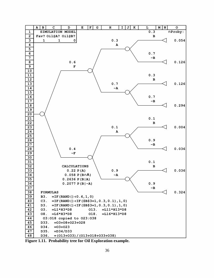
Figure 1.11 shows a tree diagram that summarizes the probability assumptions that were

used to construct the simulation model in Figure 1.10. (The simulation model is also

reconstructed in cells B3:D3 of Figure 1.11.) To read this tree diagram, you need to understand a

few basic rules that we will apply in all such probability-tree diagrams.

The circles in our probability-tree diagrams are called nodes, and the lines that go out to

the right from these nodes are called branches. Our probability-tree diagrams should be read

from left to right, and they begin at the left-hand side with one node which we may simply call

the root of the tree.

Each branch in a probability tree is assigned a label that identifies it with some event that

could occur. At each node, the branches that go out to the right from it must represent all

possible answers to some question about which we are now uncertain. That is, the branches that

go out to the right from each node must represent events that are mutually exclusive (in the sense

that at most one of them can be occur) and exhaustive (in the sense that at least one of them must

be occur). The label of each branch is shown directly above the branch in our tree diagrams.

The two branches that follow from the root of Figure 1.11 represent the two possible

answers to the question: "Do favorable strata exist in this area?" Here we use the abbreviation F

to denote the event that favorable strata exist in this area, and we let !F to denote the event that

favorable strata do not exist. In this abbreviated notation for events, a minus sign may be read as

an abbreviation for the word "not."

123456789101112131415161718192021222324252627282930313233343536373839404142434445464748

A B C D E F G H I J K L M N OSIMULATION MODEL 0.3 ∩∩∩∩Proby:

Fav? Oil@A? Oil@B? B1 1 0 0.3 0.054

A

0.7-B

0.6 0.126F

0.3B

0.7 0.126-A

0.7-B

0.294

0.1B

0.1 0.004A

0.9-B

0.4 0.036-F

0.1CALCULATIONS B

0.22 P(A) 0.9 0.0360.058 P(B∩Α∩Α∩Α∩Α) -A

0.2636 P(B|A)0.2077 P(B|-A) 0.9

-BFORMULAS 0.324B3. =IF(RAND()<0.6,1,0)C3. =IF(RAND()<IF($B$3=1,0.3,0.1),1,0)D3. =IF(RAND()<IF($B$3=1,0.3,0.1),1,0)O3. =L1*H3*D8 O13. =L11*H13*D8O8. =L6*H3*D8 O18. =L16*H13*D8O3:O18 copied to O23:O38

D33. =O3+O8+O23+O28D34. =O3+O23D35. =D34/D33D36. =(O13+O33)/(O13+O18+O33+O38)

36

Figure 1.11. Probability tree for Oil Exploration example.

37

Now go along either of the branches from the root, and you come to a second node that is

followed by two branches labelled "A" and "!A." Here A denotes the event of that oil can be

found in Tract A, so these two branches represent the two possible answers to the question: "Can

oil be found at Tract A?" Similarly, each of the four nodes in the J column is followed by two

branches labelled "B" and "!B" which represent the two possible answers (Yes and No) to the

question "Can oil be found at Tract B?" Thus, any complete path from left to right through the

tree in Figure 1.11 corresponds to one possible combination of values for our simulation model

in cells B3:D3. For example, the path from the root to the terminal triangle in cell N8 goes

through branches with labels F and A and !B, and so it represents the outcome of favorable strata

existing with oil in Tract A but not in Tract B, which corresponds to the values (1,1,0) in cells

B3:D3.

Each branch in a probability tree is assigned a probability, which we show directly above

the label in our tree diagrams. The probability that we write above any branch always denotes

the conditional probability of the branch's event given all the events on the path from the root to

the node that this branch follows. Thus, for any given node, the probabilities of the various

branches that follow this node must always add up to 1, because these branches represent

mutually exclusive and exhaustive events.

Of course, the path from the root to itself contains no events. So the probability on a

branch that goes out from the root represents the probability of the corresponding event given our

current information. In this example, we currently believe that favorable strata have probability

0.6 here, so the probability P(F) = 0.6 is shown above the upper branch from the root, while the

probability P(!F) = 1!0.6 = 0.4 appears above the lower branch from the root.

In the upper part of the tree diagram that follows after the "F" branch, notice that each of

the branches with label A or B has the probability 0.3. This is because the conditional

probability of finding oil in each tract is 0.3 given favorable strata, that is

P(A*F) = 0.3 and P(B*F) = 0.3.

But in the lower part of the tree diagram that follows after the "!F" branch, each of the branches

with label A or B has the probability 0.1, because the conditional probability of finding oil in

38

each tract is 0.1 given unfavorable strata, that is

P(A*!F) = 0.1 and P(B*!F) = 0.1.

For any two events C and D, we let C1D denote the event that C and D are both true,

which is called the intersection of these two events. So the probability at the topmost "B" branch

which follows the events F and A actually represents P(B*F1A), that is, the conditional

probability of oil at Tract B given favorable strata and oil at Tract A. Similarly, the probability

of the second highest "B" branch after A and !A represents P(B*F1!A), the conditional

probability of oil at Tract B given favorable strata and no oil at Tract A. The equality

P(B*F1A) = 0.3 = P(B*F1!A) = P(B*F)

is a result of our assumption that the events of finding oil in the two tracts would be conditionally

independent given the existence of favorable strata in this area. That is, once we know whether

favorable geological strata exist in this area, learning about oil in one tract would not affect our

beliefs about the likelihood of finding oil in the other tract.

I should now explain my initial claim that the tree in Figure 1.11 summarizes the

probability assumptions which were used to construct the simulation model in cells B3:D3. The

key is that cells in the simulation model have been constructed in the same order as their events

appear in the tree. First, in cell B3, we simulate the event of favorable strata using the

probability P(F) after the first node in the tree. Then, in cell C3, we simulate the event of oil at

Tract A using the conditional probability for this event given the results of the simulation in

cell B3, as listed in the second level of branches in the tree (the H column of Figure 1.11).

Finally, in cell D3, we simulate the event of oil at Tract B using the conditional probability for

this event given the results of the simulation in cell B3 and C3, as listed in the third level of

branches in the tree (the L column of Figure 1.11). Of course, the conditional independence of

events A and B given the event F implies that the probability of a 1 in cell D3 actually depends

only on the simulated value of cell B3, not on cell C3.

For each endpoint of a probability tree, the probability of the intersection of all events on

the path from the root to this endpoint can be computed by multiplying all the (conditional)

probabilities of all the branches on the path to this endpoint. This probability may be called the

intersection probability at this endpoint. In Figure 1.11, the intersection probabilities at all

39

endpoints have been computed in the O column. For example, in cell O3 we have

P(F1A1B) = 0.054 = 0.6*0.3*0.3 = P(F)*P(A*F)*P(B*F1A).

These intersection probabilities in Figure 1.11 are the probabilities of the eight possible outcomes

of our simulation model in cells B3:D3. Notice that, as fractions of 1000 simulations, the

frequencies found in cells L12:L19 of Figure 1.10 are indeed very close to the actual probabilities

that are shown in O3:O38 of Figure 1.11.

The (unconditional) probability of any event can be computed from such a probability

tree by adding up the intersection probabilities at all endpoints that follow paths where this event

is true. Thus, for example, the probability of finding oil at Tract A is

P(A) = P(F1A1B) + P(F1A1!B) + P(!F1A1B) + P(!F1A1!B)

= 0.054 + 0.126 + 0.004 + 0.036 = 0.22

as shown in cell D33 of Figure 1.11. Similarly, the probability of finding oil at both tracts is the

sum of the intersection probabilities at all endpoints that follow paths where A and B both occur,

that is,

P(A1B) = P(F1A1B) + P(!F1A1B) = 0.054 + 0.004 = 0.058

as shown in cell D34.

The conditional probability of any event C given any other event D is the probability of

their intersection divided by the probability of the given event D. That is,

P(C*D) = P(C1D)'P(D).

This general formula is often called Bayes's rule. In a probability tree, this formula tells us that,

to compute such a conditional probability, we should divide the sum of all endpoint intersection

probabilities where both event occur by the sum of all endpoint intersection probabilities where

the given event occurs. For example, the conditional probability of finding oil at Tract B given

that oil has been found at Tract A (when we do not know about the geological strata) is

P(B*A) = P(B1A)'P(B) = 0.058'0.22 = 0.2636

as shown in cell D35 of Figure 1.11. (Notice that B1A and A1B both denote the same

intersection of events A and B.) Similarly, to compute the conditional probability of oil at

Tract B given no oil at Tract A, we can divide the sum of intersection probabilities at endpoints

that follow both !A and B by the sum of intersection probabilities at all endpoints that

40

follow !A, that is:

P(B*!A) = P(B1!A)'P(!A) =

= (0.126+0.036)'(0.126+0.294+0.036+0.324) = 0.2077

as computed in cell D36 of Figure 1.11.

Figure 1.12 shows a second probability tree that considers only the questions of whether

oil can be found at Tract A and whether oil can be found at Tract B. The question of oil at

Tract A (the event A or !A) is considered first at the root of this tree, and then the question of oil

at Tract B is considered at the pair of nodes that follow after the A and !A branches. The

probability at the A branch here is the unconditional probability P(A) = 0.22. The probability of

the upper B branch, following A, is P(B*A) = 0.2636. The probability of the lower B branch,

following !A, is P(B*!A) = 0.2077. So all of these branch probabilities in Figure 1.12 can be

taken from our calculations of probabilities and conditional probabilities using the first tree in

Figure 1.11. For the purposes of computing the probability of any event involving A and B, this

second probability tree in Figure 1.12 is just as good as the first probability tree in Figure 1.11.

For example, cell Y3 of Figure 1.12 computes the endpoint intersection probability

P(A1B) = P(A)*P(B*A) = 0.22*0.2636 = 0.058

which is the same answer that we got from the first tree in cell D34 of Figure 1.12.

Just as the branch probabilities in the first tree were used to construct the simulation

model in cells B3:D3 of Figure 1.10, so the branch probabilities in this second tree can be used to

construct a second simulation model of these two tracts, which is shown in cells Y23:Z23 of

Figure 1.12. The key to this construction is to consider the simulated events in the same order as

they appear in the probability tree. First, in cell Y23, we simulate the answer to the question "Is

there oil at Tract A?" so that a value 1 (denoting the answer "Yes" and the event A) occurs with

the same probability P(A) that is listed above the A branch in this tree (in cell T3 of the

spreadsheet). So the formula in cell Y23 is

=IF(RAND()<T3,1,0)

Then, in cell Z23,we simulate the answer to the question "Is there oil at Tract B?" so that a

value 1 (denoting the answer "Yes" and the event B) occurs with the appropriate probability

given the simulated value of cell Y23, either P(B*A) = 0.2636 if Y23 = 1, or P(B*!A) = 0.2077

1234567891011121314151617181920212223242526272829

Q R S T U V W X Y Z AA0.2636 ∩∩∩∩Proby:

B0.22 0.058A

0.7364-B

0.162

0.2077B

0.78 0.162-A

0.7923FORMULAS -BT3. =D33 0.618T13. =1-T3W1. =D35W6. =1-W1 SIMULATION MODELW11. =D36 Oil@A? Oil@B?W16. =1-W11 1 0 Y3. =T3*W1Y8. =T3*W6Y13. =T13*W11Y18. =T13*W16Y23. =IF(RAND()<T3,1,0)Z23. =IF(RAND()<IF(Y23=1,W1,W11),1,0)

41

Figure 1.12. Alternative tree and model for Oil Exploration example.

if Y23 = 0. These two conditional probabilities appear above the appropriate branches of this

tree in cells W1 and W11 of this spreadsheet, and so the formula in cell Z23 is

=IF(RAND()<IF(Y23=1,W1,W11),1,0)

If we only care about whether oil can be found at Tracts A and B (and we do not

otherwise care about whether the deep geological strata are "favorable" or not), then these two

simulation models in Figures 1.10 and 1.12 are just as good, and they can give equally valid

estimates of any probability that involves these events A and B. In fact, if we were given a large

table of simulation data that was generated either by cells C3:D3 in Figure 1.10 or by cells

42

Y23:Z23 in Figure 1.12, there is no statistical test that could distinguish which of these two

models generated the data.

So why would we use one model rather than the other? In practice, we should use the

model that has parameters which are easier for us to assess. The second model corresponds to

the simpler probability tree in Figure 1.12, which only requires us to specify P(A), P(B*A), and

P(B*!A). (The other three branch probabilities can be computed from the basic rule that, at each

node, the sum of probabilities on branches going out to the right must equal 1.) That is, this

model requires us to ask our best expert three questions:

(1) How likely is it that oil can be found at Tract A?

(2) If you learned that oil could be found at Tract A, then how likely would you consider

oil at Tract B?

(3) If you learned that oil could be not found at Tract A, then how likely would you

consider oil at Tract B?

In an example like this one, it may be critical to recognize that finding oil at Tract A would

increase our beliefs about the probability of finding oil at Tract B. So we should not make the

error of assuming independence among these two tracts, and we need to ask the latter two

questions to differentiate P(B*A) from P(B*!A).

But although our expert should recognize that finding oil at Tract A would make us

somewhat more optimistic about finding oil at Tract B, even an expert might have difficulty

quantifying how much more optimistic. In an attempt to analyze this question, the expert might

start talking about why oil at one tract should affect our beliefs about the probability of oil at a

neighboring tract: "because it is evidence that favorable geological strata may underlie this whole

area." Such a statement would suggest that the expert might be more comfortable assessing the

parameters of the first model: the probability of favorable strata, the probability of finding oil at

any tract given favorable strata, and the probability of finding oil at any tract given unfavorable

strata. Notice that, with the assumptions of symmetry between the tracts and conditional

independence of the tracts given the underlying strata, the first probability tree actually requires

only three probability assessments, even though it has many more branches.

Probability trees are a useful way to organize our information in such problems, but they

43

become very hard to draw when there are more than a few events to consider. For example,

suppose we tried to draw a probability tree like Figure 1.11 for our salesperson example. We

would begin at the root with two branches to represent the events of Skill=Hi and Skill=Low.

Next, instead of drilling for oil at 2 tracts, we are looking for sales from 20 customers. If we

represented each customer by a column of nodes with two branches, we will have to draw a

probability tree with over 2,000,000 endpoints. To simplify matters, we might aggregate the

results from different customers and simply ask how many sales were achieved out of 20. This

will give us a tree with 42 endpoints. After the Skill=Hi branch there would be a node with

21branches to represent the outcomes of 0 sales, 1 sales, 2 sales, ..., 20 sales for a high-skilled

salesperson. Similarly, after the Skill=Lo branch, there would be another 21 branches to

represent the outcomes of 0 sales, 1 sales, 2 sales, ..., 20 sales for a low-skilled salesperson. But

even for this simplified tree, it would be rather difficult to draw all these branches on a page.

Figure 1.13 shows the essential information that would be contained in such a probability

tree for our salesperson example, but the lines of the tree diagram are omitted, which saves space

(but perhaps reduces clarity). Where the tree would begin with two branches to represent the

Skill=Hi and Skill=Low events, we list these events and their probabilities in the A column of

Figure 1.13. The probability P(Skill=Hi) is entered into cell A3, and the probability

P(Skill=Low) is entered into cell A27. Next, after each level of skill, the tree would have 21

branches for the possible numbers of sales from 0 to 20. These possible numbers of sales are

listed in cells B3:B23 for the Skill=Hi case, and in cells B27:B47 for the Skill=Low case.

1234567891011121314151617181920212223242526272829303132333435363738394041424344454647

A B C D E F GSkill=Hi [P(Sale)=2/3 in each call]P(Skill) k P(Sales=k|Skill) Product P(Skill=Hi|Sales=k)

0.5 0 0.0000 0.0000 0.00001 0.0000 0.0000 0.00002 0.0000 0.0000 0.00003 0.0000 0.0000 0.00014 0.0000 0.0000 0.00025 0.0001 0.0001 0.00106 0.0007 0.0004 0.00397 0.0028 0.0014 0.01548 0.0092 0.0046 0.05889 0.0247 0.0123 0.2000

10 0.0543 0.0271 0.500011 0.0987 0.0493 0.800012 0.1480 0.0740 0.941213 0.1821 0.0911 0.984614 0.1821 0.0911 0.996115 0.1457 0.0729 0.999016 0.0911 0.0455 0.999817 0.0429 0.0214 0.999918 0.0143 0.0071 1.000019 0.0030 0.0015 1.000020 0.0003 0.0002 1.0000

Skill=Lo [P(Sale)=1/3 in each call]P(Skill) k P(Sales=k|Skill) Product FORMULAS

0.5 0 0.0003 0.0002 C3. =BINOMDIST(B3,20,2/3,0)1 0.0030 0.0015 D3. =$A$3*C32 0.0143 0.0071 C3:D3 copied to C3:D233 0.0429 0.0214 A27. =1-A34 0.0911 0.0455 C27. =BINOMDIST(B27,20,1/3,0)5 0.1457 0.0729 D27. =$A$27*C276 0.1821 0.0911 C27:D27 copied to C27:D477 0.1821 0.0911 F3. =D3/(D3+D27)8 0.1480 0.0740 F3 copied to F3:F239 0.0987 0.0493

10 0.0543 0.027111 0.0247 0.012312 0.0092 0.004613 0.0028 0.001414 0.0007 0.000415 0.0001 0.000116 0.0000 0.000017 0.0000 0.000018 0.0000 0.000019 0.0000 0.000020 0.0000 0.0000

44

Figure 1.13. Binomial probability computations for Salesperson example.

45

To complete the description of the probability tree, we need to specify the conditional

probabilities that would be associated with these 42 branches. That is, for each number k from 0

to 20, we need the conditional probabilities P(k sales*Skill=Hi) and P(k sales*Skill=Low).

Finding these conditional probabilities is the essence of the problem, and much of our work in

Section 1.2 was essentially showing how these conditional probabilities could be estimated from

a simulation model. But such questions have been considered by many mathematicians before,

and they have developed a theory of Binomial distributions that can be used to directly compute

probabilities in this specific kind of situation. I have not stressed this theory here, because I want

to emphasize modeling skills that you can apply to more general kinds of problems. But some

readers may have studied Binomial distributions in another course, so let me say briefly how they

can be applied here.

Binomial-distribution theory tells us that, if there will be n independent trials (for some

given number n), and the probability of a "success" in each trial will be p (for some given

probability p), and the result of each trial will be independent of all other trials, then the

probability of getting exactly k successes in n trials is given by a specific formula which is

returned by the Excel function

BINOMDIST(k,n,p,0)

This (magical) formula is applied in column C of Figure 1.13. The number of trials is n=20.

These trials are not independent when the salesperson's skill is unknown, and so the Binomial

theory could not be applied without knowing the skill. But if we are given that Skill=Hi, then the

trials (calls on different customers) become independent with a probability of success (a sale)

being 2/3 in each trial. So the probabilities P(k sales*Skill=Hi) are computed, for all the various

values of k in B3:B23, by entering the formula

=BINOMDIST(B3,20,2/3,0)

into cell C3, then and copying C3 to C3:C23. Similarly, if we are given that Skill=Low, then the

trials also become independent, but now the probability of success is only 1/3 in each trial, and so

the probabilities P(k sales*Skill=Low) are computed, for all the various values of k in B27:B47,

by entering the formula

46

=BINOMDIST(B27,20,1/3,0)

into cell C27, then and copying C27 to C27:C47.

The intersection probabilities at the endpoints of this probability tree would just be the

first branch's probability (0.5 in each case) multiplied by the Binomial conditional probability in

the C column of Figure 1.13. These intersection probabilities are computed in the D column of

Figure 1.13. For example, cell D12 computes

P(Sales=9 1 Skill=Hi) = P(Skill=Hi)*P(Sales=9*Skill=Hi)

= 0.5*0.0247 = 0.0123

Similarly, cell D36 computes

P(Sales=9 1 Skill=Low) = P(Skill=Low)*P(Sales=9*Skill=Low)

= 0.5*0.0987 = 0.0493.

To compute conditional probability of Skill=Hi given Sales=9, we divide the probability of the

outcome Sales=91Skill=Hi by the sum of probabities of all outcomes where Sales=9. That is,

P(Skill=Hi*Sales=9) =

= P(Sales=91Skill=Hi)'(P(Sales=91Skill=Hi) + P(Sales=91Skill=Low))

= 0.0123'(0.0123 + 0.0493) = 0.2000

This result is computed in cell F12 of Figure 1.13 by the formula =D12/(D12+D36).

Copying this formula to D3:D23 yields the correct answer to questions that we were trying to

estimate in Sections 1.2 and 1.3 above. In particular, comparing cells D3:D23 in Figure 1.13 to

cells L35:L55 in Figure 1.7, you can see how accurate our simulation estimates were.

It is very nice to be able to have this special BINOMDIST formula that enables us to

compute these conditional probabilities exactly. But special formulas require special structures

that restrict the class of models that we can consider. In contrast, the methods of simulation

analysis can be extended to virtually any case of decision-making under uncertainty. This

generality is the main reason why this book emphasizes simulation analysis as a unifying

analytical methodology. Some inexactness of results is a small price to pay for the great

generality of practical applications that we will be able to address.

47

*1.7. Advanced spreadsheet techniques: constructing a table with multiple inputs

Figure 1.14 shows how the simulation model of Figure 1.10 was analyzed, to generate the

table of simulation results, which appeared in cells B13:E20 of Figure 1.10 but appear in cells

I13:L20 of Figure 1.14. Figure 1.14 looks complicated, but you should recognize that there are

really three basic parts of this spreadsheet. First, the range B3:D3 of this spreadsheet contains

the simulation model for our oil-exploration example. Second, below the model, we have

generated a simulation table that contains data from 1000 recalculations of this model, stored in

the range B4:D1003. Only the top 30 rows of data are shown in Figure 1.14, but the SimTable

data continues in the spreadsheet down to row 1003. Third, in columns F through L, we have a

data-analysis section that serves to extract basic summary statistics from our simulation data. Let

me now explain how this analytical section works, because it applies some advanced techniques

that you may find useful later.

The cells in the F column of Figure 1.14 are designed to count how many simulation

outcomes match the pattern shown in the range I1:K1 (currently 1,1,1). Cell F4 contains the

formula

=IF(AND(B4=$I$1,C4=$J$1,D4=$K$1),1,0)

and cell F4 has been copied to F4:F1003. Here we use Excel's AND function, which takes any

number of true-or-false propositions as inputs and returns the value "TRUE" if all of these inputs

are true, but returns the value "FALSE" if any of these inputs are not true. So if the three values

in B4:D4 exactly matched the corresponding values in I1:K1, then the expression

AND(B4=$I$1, C4=$J$1, D4=$K$1)

would be TRUE, which would make cell F4 take the value 1. But otherwise, if any cell in B4:D4

is different from the corresponding cell in I1:K1, then this AND expression must be FALSE and

the value of cell F4 must be 0.

1234567891011121314151617181920212223242526272829303132

A B C D E F G H I J K L M NSIMULATION MODEL Total 1 1 1 1

FavStr? Oil@A? Oil@B? 56 Index Pattern SimTable 1 0 1 =I1:K1? 1 1 1 1

0 0 0 0 0 2 1 1 00.001001 1 0 0 0 3 1 0 10.002002 1 0 0 0 4 1 0 00.003003 1 0 1 0 5 0 1 10.004004 0 0 0 0 6 0 1 00.005005 0 0 0 0 7 0 0 10.006006 1 1 1 1 8 0 0 00.007007 1 0 1 00.008008 1 0 1 0 FavStr? Oil@A? Oil@B? Frequency0.009009 0 1 1 0 1 Yes Yes Yes 560.01001 1 1 0 0 2 Yes Yes No 129

0.011011 1 1 0 0 3 Yes No Yes 1410.012012 1 1 0 0 4 Yes No No 2840.013013 0 0 0 0 5 No Yes Yes 30.014014 0 0 0 0 6 No Yes No 370.015015 1 0 0 0 7 No No Yes 320.016016 1 0 0 0 8 No No No 3180.017017 0 0 0 00.018018 1 0 1 0 FORMULAS0.019019 0 0 1 0 B3. =IF(RAND()<0.6,1,0)0.02002 1 0 0 0 C3. =IF(RAND()<IF($B$3=1,0.3,0.1),1,0)

0.021021 1 1 0 0 D3. =IF(RAND()<IF($B$3=1,0.3,0.1),1,0)0.022022 0 0 0 0 F4. =IF(AND(B4=$I$1,C4=$J$1,D4=$K$1),1,0)0.023023 1 0 1 0 F4 copied to F4:F10030.024024 0 0 0 0 F2. =SUM(F4:F1003)0.025025 1 0 0 0 I1. =INDEX(I3:I10,$H$1) I1 copied to I1:K10.026026 1 1 0 0 I13. =IF(I1=1,"Yes","No") I13 copied to J13:K130.027027 1 1 1 1 L13. =F2 H13. =H10.028028 1 1 1 1 I14:L20. {=TABLE(,H1)}

48

Figure 1.14. Computing frequencies of different outcomes in Oil Exploration example.

49

Because the dollar signs in cell F4 of Figure 1.14 make the references to I1:K1 absolute

constants in the copying process, each cell in F4:F1003 takes the value 1 if the B:D cells in its

row are all the same as the pattern in I1:K1, and it takes the value 0 otherwise. Then cell F2

contains the formula

=SUM(F4:F1003)

and so it displays the total number of rows where the B:D cells match the pattern in I1:K1. With

value 1 in each of the cells of the pattern range I1:K1, the value 56 in cell F2 tells us that, among

the 1000 simulations that are stored in this table, there were exactly 56 simulations in which the

outcome was favorable strata with oil in both tracts (including rows 10, 31, and 32 shown here).

Now if we change the spreadsheet in Figure 1.14 by putting different combinations of

zeroes and ones in the pattern range I1:K1, we can find in cell F2 the total number of times that

each possible outcome occurred. These results (with the interpretation that 1 means "Yes" and 0

means "No" in our simulation data) are shown in cells I13:L20 of Figure 1.14. For example, cell

L14 tells us that there were 129 rows (including rows 14, 15, 16, 25, and 30) where the

simulation outcome was (1,1,0), which represents the event that favorable strata exist in this area,

and there is oil in Tract A, but there is no oil in Tract B.

The statistical summary in cells I13:L20 of Figure 1.14 was generated by changing the

values in I1:K1. Because there are only 2*2*2 = 8 possible combinations of zeroes and ones to

be tried in this three-cell range, it is not too tedious to make these substitutions by hand.

However, you might want to know how this process was accomplished automatically in this

spreadsheet.

The range I3:K10 in Figure 1.14 lists, in its eight rows, all eight possible combinations of

zeroes and ones that could be entered into our three-cell pattern I1:K1. (Simtools.xla provides a

"CombineRows" procedure that can be used to automatically generate tables of all combinations,

such as we have in I3:K10 here. But these 8 combinations here are easy enough to generate by

hand, and we will not have further use of this feature, so its discussion is omitted.) Now we want

to automatically force the spreadsheet to re-evaluate the total in cell F2 as each of these rows is

substituted into the pattern range I1:K1.

When we need to re-evaluate a spreadsheet with different values substituted into a cell,

50

we can do it with a column-input data table. But how can we re-evaluate a spreadsheet with

different values being substituted into three cells? The trick is to set up these three cells so that

their values are controlled by one cell, and then let that one cell be the column-input cell of our

data table.

In Figure 1.14, the cell I1 contains the formula

=INDEX(I3:I10,$H$1)

and this formula (with its absolute reference to $H$1) has been copied to cells J1 and K1. Given

a range of cells in one column as its first parameter and given a number as its second parameter,

Excel's INDEX function returns the value of the cell in the given range that is indicated by the

given number, counting the top cell as number 1, the second cell as number 2, and so on. So

when H1 equals 1, the cells I1:K1 take their values from the corresponding cells in the top row of

I3:K10 (that is I3:K3). But if the value of H1 were changed to 2, then cells I1:K1 would take

their values from the second row of I3:K10, which are (1,1,0) in cells I4:K4, and then cell F2

would be counting the number of simulations where favorable strata occurred with oil at Tract A

but not at Tract B. So by changing the value of H1 from 1 to 8, we can set the values of I1:K1

equal to each of the possible combinations that are listed in the rows of I3:K10.

Now we are ready to explain how the statistical table in cells I13:L20 of Figure 1.14 was

generated. In the top row of this range, the I:K cells repeat the pattern range I1:K1, except that

they translate a 1 to a "Yes" and a 0 to a "No". The formula in cell I13 is

=IF(I1=1,"Yes","No")

and this formula has been copied to J13 and K13. Cell L13 contains the formula =F2, so L13

simply repeats the statistical count of pattern-matches that we computed in cell F2. Then the

range I14:L20 below these cells has been filled by a column-input data table, which shows how

the values of I13:L13 would change if the corresponding inputs at left (the numbers 2, 3, 4, ..., 8

in cells H14:H20) were substituted into our index-control cell H1. That is, the cells I14:L20 are

filled with the formula {=TABLE(,H1)}, which was created by selecting H13:L20 and then

using the Data:Table menu command, with H1 as the column-input cell.

51

1.8 Using models

We have introduced several models in this chapter, and we will see many more in the rest

of this book. So it may be helpful to have a few general remarks about how models are used.

A model of a complex system is just a simpler and more accessible system that is in some

ways like the complex system, so that we can try to learn about the complex system's properties

by doing experiments with the model. Every model is a simplification, omitting many of the true

complexities of the world that it is intended to describe. The only model that could ever be

exactly like the real world in every aspect would be the real world itself, and if we denied the

relevance of any other models then we could make no prediction about the results of any decision

until it was actually implemented.

This book is about formal quantitative models in spreadsheets. But of course there are

many other kinds of models. Even when you think informally about some situation in which you

have to make a decision, you are creating a model of this situation in your head, as you imagine

how your decision might affect the various consequences that you care about. The model in your

imagination is a simplification of reality, just as a spreadsheet model is, and neither model is

necessarily better or more accurate.

One advantage of formal quantative models is that their details are completely specified

in a way that other people can examine and discuss. Indeed, the task of constructing a

quantitative model can be divided among various members of a team, giving each person

responsibility for making the parts of the model that he knows best. In contrast, the model of

your imagination must be in your mind alone, where it is not so transparent to others, and so it is

harder for you to ask friends or teammates to help scrutinize the hidden assumptions of your

thoughts. There will always be questionable simplifying assumptions in any model, but in a

formal model these assumptions are out in the open for examination by anyone who knows how

to read it. When an important applied decision is to be based on the analysis of a formal

quantitative model, we should always check to see how our conclusions might change when

some of the model's questionable assumptions are changed. This process is called sensitivity

analysis.

A disadvantage of formal quantitative models is that they may encourage us to focus only

52

on those aspects of the situation that are quantitively measurable. Furthermore, nothing goes into

a formal model until we focus on it and consciously enter it into some part of the model. In

contrast, the informal models of your imagination may draw almost effortlessly on your

memories from many different experiences in life, possibly including some memories of which

you are not even conscious, in which case the results of your thought process may be called

"intuition." So it is important to compare the results of a formal quantitative model with our

intuition about the situation. When the results of a formal quantitative model contradict our

intuition, we should ask whether there is some important factor that the model has omitted and

that is the basis of our intuition. If so, then we must try to extend the formal model to take this

factor into account.

In this sense, applied formal modeling work should always done in a dialogue with our

intuition. The formal model can help us to see connections that we might not have recognized,

but our intuition may point out features that are missing in the model. Thus, although we must

accept that our models will always be incomplete simplifications of reality, we must always be

prepared to make them more complete (and less simple) when intuition suggests that something

important may be missing.

We have seen in this chapter that there may be more than one useful way to model any

real situation, and that a decision-maker may want to compare different models in terms of how

well they describe what is actually known about about the real situation. For example, the model

of the new salesperson in Figure 1.4 was extended to a more complex model in Figure 1.9, which

a manager might consider a better description of this situation. In Chapter 6 (Figure 6.1) we will

introduce yet another model which might be an even better fit to the manager's intuitive

understanding of the situation. In Figures 1.10 and 1.13 we saw two simple models that are

mathematically equivalent, in the sense that they make identical predictions about the

probabilities of finding oil in these tracts. Such equivalent models must be considered equally

accurate as descriptions of the actual situation, but they may differ in terms of which is more

convenient to use.

In any quantitative model, there are some parameters that must be assessed or measured

from the real situation, and then the model can be used to compute estimates of other quantities

53

that a decision-maker might want to know. But different models of the same situation may differ

in terms of which quantities are assessed in building the model, and which other quantities can be

computed from the model. The most convenient model is the one that has parameters which are

easiest for the decision-maker to assess, and that can be used to compute all the other quantities

that are important to the decision-maker.

Some parameters in a quantitative model may be very difficult to measure or assess

accurately. For example, sellers of some product may not know exactly how many units of this

product will be demanded by their customers next year. They may feel that this unknown

quantity of demand could be any number within some range of uncertainty. When this range of

uncertainty is small, a modeler might just pick some number in this range as a good guess of the

quantity, and might analyze the model as if there were no uncertainty about this guess. But then

the modeler should do sensitivity analysis to see how results might change with other reasonable

guesses of this unknown quantity. When the range of uncertainty is large, so that sensitivity

analysis suggests that the different reasonable guesses would imply substantially different

optimal decisions, then we really need to use models that express our uncertainty.

As we have seen, uncertainty is expressed in quantitative models by using probabilities.

When we feel unable to accurately assess some quantity, like next year's demand, we can instead

try to assess the probabilities of different possible values of this quantity. For example, when we

cannot say whether next year's demand for our product will be more than 5000 units, we may

instead talk about the probability of this demand being more than 5000 units, to describe how

likely such outcomes might be. The art of making and using models with probabilities is the

subject of this book.

1.9. Summary

This chapter focused on an example in which we want to learn about some unknown

quantity (a salesperson's level of skill) by observing other events (the successes and failures in

various sales calls) that are influenced by this unknown quantity. We analyzed this problem

using spreadsheet simulation models in which one random cell simulates the unknown quantity

and other cells simulate the observations that depend on the unknown quantity.

54

In the context of this problem, we introduced some basic ideas of probability, including:

prior probabilities and conditional probabilities P(A*B), independence and conditional

independence, and Uniform and Triangular probability distributions. We saw how various

conditional probabilities can be used to construct a randomized (Monte Carlo) simulation model,

and how data from such a model can then be used to estimate other conditional probabilities. In

general, the conditional probability of any event A given any other event B satisfies the equation

P(A*B) = P(A1B)'P(B)

This formula implies that, to estimate P(A*B) from data of many independent simulations, the

number of simulations in which A and B both happened together should be divided by the total

number of simulations in which B happened (with or without A). A second example about

drilling for oil in two tracts was used to illustrate how conditional probabilities can also be

computed directly from other conditional probabilities in a probability-tree diagram.

This chapter introduced basic keystroke techniques for doing such simulation analysis in

spreadsheets, using Excel with the Simtools add-in. Excel functions introduced here include:

RAND, IF, COUNT, SUM, AVERAGE, PERCENTRANK, PERCENTILE, BINOMDIST,

AND, INDEX, and we also introduced the Simtools function TRIANINV. We saw how to get

information about these and other technical functions in Excel, by the using of the

Insert:Function dialogue box. Other basic spreadsheet techniques that were reviewed in this

chapter include: copying and pasting with absolute ($) and relative references in formulas,

simulation tables, and column-input data tables.

The RAND() function is the heart of all simulation models, because every RAND()

formula returns an independent random variable drawn from the Uniform distribution between 0

and 1. Thus, if x and y are numbers such that 0 # x # y # 1, then the probability of any RAND()

being between x and y (after the next recalculation of the spreadsheet) is just the difference y!x.

That is,

P(x # RAND() # y) = y ! x.

To compute conditional probabilities from large tables of simulation data, we used a

formula-filtering technique in which a column is filled with IF formulas that extract information

from a simulation table, returning a nonnumerical value ("..") in data rows that do not match our

55

criterion. The information extracted in such columns can be summarized using statistical

functions like COUNT, SUM, AVERAGE, PERCENTRANK, and PERCENTILE, which are

designed to ignore nonnumerical entries.

EXERCISES

1. The Connecticut Electronics company produces sophisticated electronic modules in

production runs of several thousand at a time.. It has been found that the fraction of defective

modules in can be very different in different production runs. These differences are caused by

micro-irregularities that sometimes occur in the electrical current. For a simple first model, we

may assume first that there are just two possible values of the defective rate.

In about 70% of the production runs, the electric current is regular, in which case every module

that is produced has an independent 10% chance of being defective.

In the other 30% of production runs, when current is irregular, every module that is produced has

an independent 40% chance of being defective.

Testing these modules is quite expensive, so it is valuable to make inferences about the overall

rate of defective output based on a small sample of tested modules from each production run.

(a) Make a spreadsheet model to study the conditional probability of irregular current given the

results of testing 10 modules from a production run. Make a simulation table with data from at

least 1000 simulations of your model (where each simulation includes the results of testing 10

modules), and use this table to answer the following questions.

(b) What is the probability of finding exactly 2 defective modules among the 10 tested?

(c) What is the conditional probability that the current is regular given that 2 defective modules

are found among the 10 tested?

(d) Make a table showing the estimates of P(irregular current| k defectives among 10 tested), for

k = 0, 1, 2,... (You may have trouble with some k greater than 7, but the answer in those cases

should be clear.)

2. Reconsider the Connecticut Electronics problem, but let us now drop the assumption that

each run's defective rate must be one of only two possible values. Managers have observed that,

due to differences in the electrical current, the defective rate in any production run may be any

number between a lower bound of 0% and an upper bound of 50%. They have also observed that

the defective rates are more likely to be near 10% than any other single value in this range. So

suppose that the defective rate on any production run is drawn from a Triangular distribution

with these parameters. We want to quantify what we can infer about the defective rate in the

most recent production run based on the testing of ten modules from this production run.

56

(a) Before we test any modules, what is the probability of a defective rate less than 0.25 in this

production run? For what number M would you say that the defective rate is equally likely to be

above or below M?

(b) Based on data from at least 1000 simulations, what is the probability that we will find exactly

2 defective modules when we test ten modules from this production run?

(c) Suppose that we found exactly 2 defective modules when we tested ten modules from this

production run. Given this observation, what is the conditional probability of a defective rate

less than 0.25 in this production run? For what number M would you say that the defective rate

in this production run is equally likely to be above or below M?

(d) How would your answers to part (c) change if we found 0 defective modules when we tested

ten modules from this production run?

3. Consider again our basic model of the salesperson who makes 20 sales-calls. Before he

makes these calls, we think that he is equally likely to have high skill or low skill. If he has high

skill, then his probability of making a sale is 2/3 in each call. If he has low skill, then his

probability of making a sale is 1/3 in each call. We consider the results of these 20 calls to be

conditionally independent given his skill.

(a) Suppose that we have a policy of promoting the salesperson if he makes at least 9 sales in

these 20 calls. Based on data from at least 1000 simulations, estimate the following

probabilities:

(a1) the probability that he will be promoted under this policy,

(a2) the conditional probability that he will be promoted under this policy if he has high skill,

(a3) the conditional probability that he has high skill given that he is promoted under this

policy.

(b) Make a table showing the how the three probabilities that you computed in part (a) would

change if the policy were instead to promote the salesperson if he makes at least n sales in the 20

calls, for any integer n between 0 and 20.

4. Another oil-exploration company is negotiating for rights to drill for oil in Tracts C and D

which are near each other (but in a very different area of the world from the Tracts A and B that

were discussed in Section 1.6). The company's geological expert has estimated that the

probability of finding oil at Tract C is 0.1. He has also estimated that the conditional probability

of oil at Tract D given oil at Tract C would be 0.4. Finally, he has also estimated that the

conditional probability of oil at Tract D given no oil at Tract C would be 0.02.

(a) Using the expert's probability assessments, compute the probability of oil at Tract D, and

compute the conditional probability of oil at Tract C given oil at Tract D.

57

(b) Suppose that the expert asserts that oil at Tract D is just as likely as oil at Tract C. This

assertion suggests that at least one of his three assessments above must be wrong. Suppose that

he feels quite confident about his estimate of the probability of C and his estimate of the

conditional probability of oil at D given oil at C. To be consistent with this new assertion, how

would he have to change the conditional probability of oil at D given no oil at C?

5. Gates & Associates regularly receives proposals from other companies to jointly develop new

software programs. Whenever a new proposal is received, it is referred to Gates's development

staff for a study to estimate whether the software can be developed as specified in the proposal.

In staff reports, proposals are rated as "good" or "not good" prospects. When the development

staff evaluates a proposal that is actually feasible, the probability of their giving it a "good"

evaluation is 3/4. When the development staff evaluates a proposal that is actually not feasible,

the probability of their giving it an "not good" evaluation is 2/3.

Proposals can also be referred to an outside consultant to get a second independent

opinion on feasibility of the proposal. In the consultant's reports, proposals are rated as "highly

promising" or "not highly promising". When the outside consultant evaluates a proposal that is

actually feasible, the probability of her giving it a "highly promising" evaluation is 0.95. When

the outside consultant evaluates a proposal that is actually not feasible, the probability of her

giving it a "not highly promising" evaluation is 0.55. Suppose that the reports of the

development staff and the outside consultant on a proposal would be conditionally independent,

given the actual feasiblity or infeasibility of the proposal.

A new proposal has just come in from Valley Software, a company that has generated

some good ideas but also has also made more than their share of exaggerated promises. Without

any technical evaluation of this new proposal, based only on Valley Software's past record, Gates

currently figures that the probability of the Valley proposal being feasible is 0.35 .

(a) Make a probability tree to represent this situation.

(b) What is the probability that the staff will report that the Valley proposal is "good"?

(c) What is the probability that the outside consultant would report that the Valley proposal is

"highly promising"?

(d) What is the conditional probability that the Valley proposal is feasible if the staff reports that

it is "good"?

(e) What is the conditional probability that the outside consultant would report that the Valley

proposal is "highly promising", if the staff reports that the proposal is "good"?

(f) If the staff reports that the Valley proposal is "good" and the outside consultant also reports

that it is "highly promising", then what is the probability that the proposal is feasible?

(g) Make a spreadsheet model that simulates this situation, where cell B3 simulates the

58

feasibility of the Valley proposal (1=feasible, 0=unfeasible), cell C3 simulates the staff report

(1=good, 0= not good), and cell D3 simulates the outside consultants report (1=highly promising,

0=not highly promising).

*(h) How might you make a model that is equivalent to the one in part (g), except that the

dircetion of influence between cells B3 and C3 is reversed? (That is, if the formula in cell C3

referred to cell B3 in your answer to part (g), then you should now make cell B3 refer to cell C3

and, to avoid circular references, cell C3 must not refer to cell B3.)

6. Random Press is deciding whether to publish a new probability textbook. Let Q denote the

unknown fraction of all probability teachers who would prefer this new book over the classic

textbook which you are now reading.

If the editor at Random knew Q, then she would say that every teacher has a conditionally

independent Q probability of preferring this new book.

Unfortunately, the editor does not know Q. In fact, the editor's uncertainty about Q can be

represented by uniform distribution over the interval from 0 to 1. That is, up to any given

number of digits, the editor thinks that Q is equally likely to be any number between 0 and 1.

To get more information about Q, the editor has paid 8 randomly sampled probability teachers to

carefully read this new book and compare it to the above-mentioned classic textbook. Three

months from now, each of these teachers will send the editor a report indicating whether he or

she would prefer this new book.

(a) Make a spreadsheet model to simulate the editor's uncertainty about the unknown fraction Qand the results that she will get from her sample of eight readers. Make a table of data from at

least 1000 simulations of your model to answer the following questions.

(b) Estimate the conditional probability that Q>.5 (that is, a majority in the overall population

will prefer the new book) given that 6 out the eight sampled prefer the new book.

(c) Estimate the conditional median value of Q given that 6 out the eight sampled prefer the new

book.

(d) Make a table indicating, for each number k from 0 to 8:

(d1) the conditional median value for Q given that k out of the eight sampled teachers prefer

the new book (that is, the number q such that P(Q<q*k prefer the new book) = 0.50);

(d2) the conditional 0.05-percentile for Q given that k out of eight prefer the new book (that

is, the number q such that P(Q<q*k prefer new book) = 0.05); and

(d3) the conditional 0.95-percentile for Q given that k out of eight prefer the new book (that

is, the number q such that P(Q<q*k prefer new book) = 0.95).

7. A student is applying 9 graduate schools. She knows that they are all equally selective, but

59

she figures that there is an independent random element in each school's selection process, so by

applying to more schools she has a greater probability of getting into at least one.

She is uncertain about her chances partly because she is uncertain about what kinds of

essays might be distinctively impressive, in the sense of being able to attract the attention of

admissions officers who read many hundreds of essays per year. Given the rest of her

credentials, the student believes that, if her application essay was distinctively impressive then, at

each school, she would have a probability 0.25 of being admitted, independently of how the other

schools responded to her application. But if she knew that her application essay was not

distinctively impressive, then she would figure that, at each school, she would have a probability

0.05 of being admitted, independently of how the other schools responded to her application.

Because of her uncertainty about what kind of essay would be distinctively impressive to

admissions officers, she has actually drafted two different application essays. Essay #1 focuses

on her experiences in the Peace Corps after college, while essay #2 focuses on her experiences as

head of the student laundry services during college. If either essay really is distinctively

impressive, then it would have this intrinsic property wherever it was sent. She does not feel sure

about the quality of either essay, but she is more optimistic about essay #1. In her beliefs, there

is probability 0.5 that essay #1 is a distinctively impressive essay, and there is probability 0.3 that

essay #2 is a distinctively impressive essay, each independently of the other.

Although she would be very glad to attend any of these 9 schools, the student considers 3

of the schools to be somewhat less preferred than the other 6, because of their geographical

locations. So she has definitely decided to use essay #1 in the applications to her 6 more-desired

schools. But she is undecided about what to do with the applications for the 3 less-desired

schools: she could use the same essay #1 for these 3 schools as well, or instead she could use

essay #2 in her applications to these 3 schools.

(a) Build a simulation model to study this situation. You can use data from at least 1000

simulations to estimate answers to the following questions (b)-(f).

(b) What is the probability that she will be rejected by all of her 6 more-desired schools when

she uses essay #1 in each of these applications?

(c) What would be the conditional probability of essay #1 being distinctively impressive given

that she was rejected by all of the 6 more-desired schools?

(d) If she also used essay #1 in her applications to the 3 less-desired schools, then what would be

her conditional probability of getting accepted by at least one of these 3 schools with essay #1

given that she was rejected by all of the 6 more-desired schools?

(e) If she instead used essay #2 in the applications to the 3 less-desired schools, then would be

her conditional probability of getting accepted by at least one of these 3 schools with essay #2,

given that she was rejected by all of the 6 more-desired schools (with the other essay)?

60

8. Consider again the oil-exploration example in Section 1.6.

(a) Compute the conditional probability of favorable strata given that neither Tract A nor Tract B

has any oil.

(b) Compute the conditional probability of favorable strata given that exactly one of the two

tracts has oil.

(c) Compute the conditional probability of favorable strata given that both of the two tracts have

oil.

(d) Make a probability tree with three levels of branches that represents this oil-exploration

example, such that the first two levels are the same as in Figure 1.12, and the third-level branches

represent the events of favorable strata existing or not existing in this area.

(e) In Figure 1.12, what formula could you enter into cell X23 to simulate "Favorable Strata?" so

that cells X23:Z23 would be a simulation model that is mathematically equivalent to the

simulation model in cells B3:D3 of Figures 1.10? (To make this model in X23:Z23, you may

also enter formulas into other blank cells of this spreadsheet, but do not change the formulas in

cells Y23 and Z23.)