106
1 Queuing Queuing Models Models Chapter 9
| Date post: | 15-Dec-2015 |
| Category: |
Documents |
| Upload: | bennett-derricott |
| View: | 231 times |
| Download: | 0 times |

1
Queuing ModelsQueuing ModelsQueuing ModelsQueuing Models
Chapter 9
2
9.1 Introduction9.1 Introduction
• Queuing is the study of waiting lines, or queues.• The objective of queuing analysis is to design
systems that enable organizations to perform optimally according to some criterion.
• Possible Criteria– Maximum Profits.
– Desired Service Level.
3
9.1 Introduction9.1 Introduction
• Analyzing queuing systems requires a clear understanding of the appropriate service measurement.
• Possible service measurements– Average time a customer spends in line.– Average length of the waiting line.– The probability that an arriving customer must wait
for service.
4
9.2 Elements of the Queuing Process9.2 Elements of the Queuing Process
• A queuing system consists of three basic components:– Arrivals: Customers arrive according to some arrival
pattern.
– Waiting in a queue: Arriving customers may have to wait in one or more queues for service.
– Service: Customers receive service and leave the system.
5
The Arrival ProcessThe Arrival Process
• There are two possible types of arrival processes
– Deterministic arrival process.
– Random arrival process.• The random process is more common in
businesses.
6
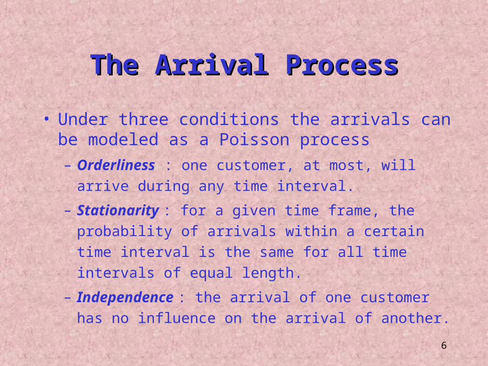
• Under three conditions the arrivals can be modeled as a Poisson process– Orderliness : one customer, at most, will arrive during any
time interval.
– Stationarity : for a given time frame, the probability of arrivals within a certain time interval is the same for all time intervals of equal length.
– Independence : the arrival of one customer has no influence on the arrival of another.
The Arrival ProcessThe Arrival Process
7
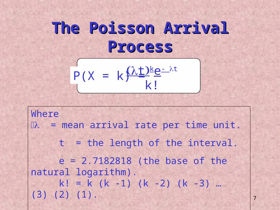
P(X = k) =
Where = mean arrival rate per time unit.
t = the length of the interval.
e = 2.7182818 (the base of the natural logarithm).k! = k (k -1) (k -2) (k -3) … (3) (2) (1).
tke- t
k!
The Poisson Arrival ProcessThe Poisson Arrival Process
8
HANK’s HARDWARE – HANK’s HARDWARE – Arrival ProcessArrival Process
• Customers arrive at Hank’s Hardware according to a Poisson distribution.
• Between 8:00 and 9:00 A.M. an average of 6 customers arrive at the store.
• What is the probability that k customers will arrive between 8:00 and 8:30 in the morning (k = 0, 1, 2,…)?
9
k
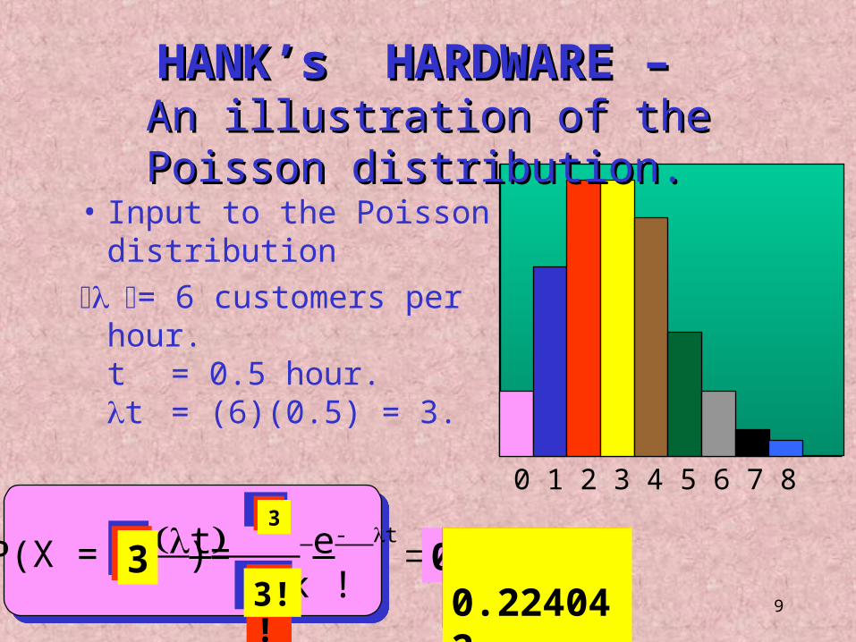
• Input to the Poisson distribution
= 6 customers per hour.t = 0.5 hour.t = (6)(0.5) = 3.
t e- t
k !
0
0.049787
0
1!
1
0.1493612
2!0.224042
3
3! 0.224042
1 2 3 4 5 6 7
P(X = k )=
8
123
HANK’s HARDWARE – HANK’s HARDWARE – An illustration of the Poisson distribution. An illustration of the Poisson distribution.
10
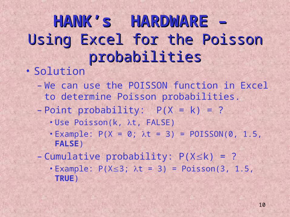
HANK’s HARDWARE – HANK’s HARDWARE – Using Excel for the Poisson probabilitiesUsing Excel for the Poisson probabilities
• Solution– We can use the POISSON function in Excel to
determine Poisson probabilities.– Point probability: P(X = k) = ?
• Use Poisson(k, t, FALSE)• Example: P(X = 0; t = 3) = POISSON(0, 1.5, FALSE)
– Cumulative probability: P(Xk) = ?• Example: P(X3; t = 3) = Poisson(3, 1.5, TRUE)
11
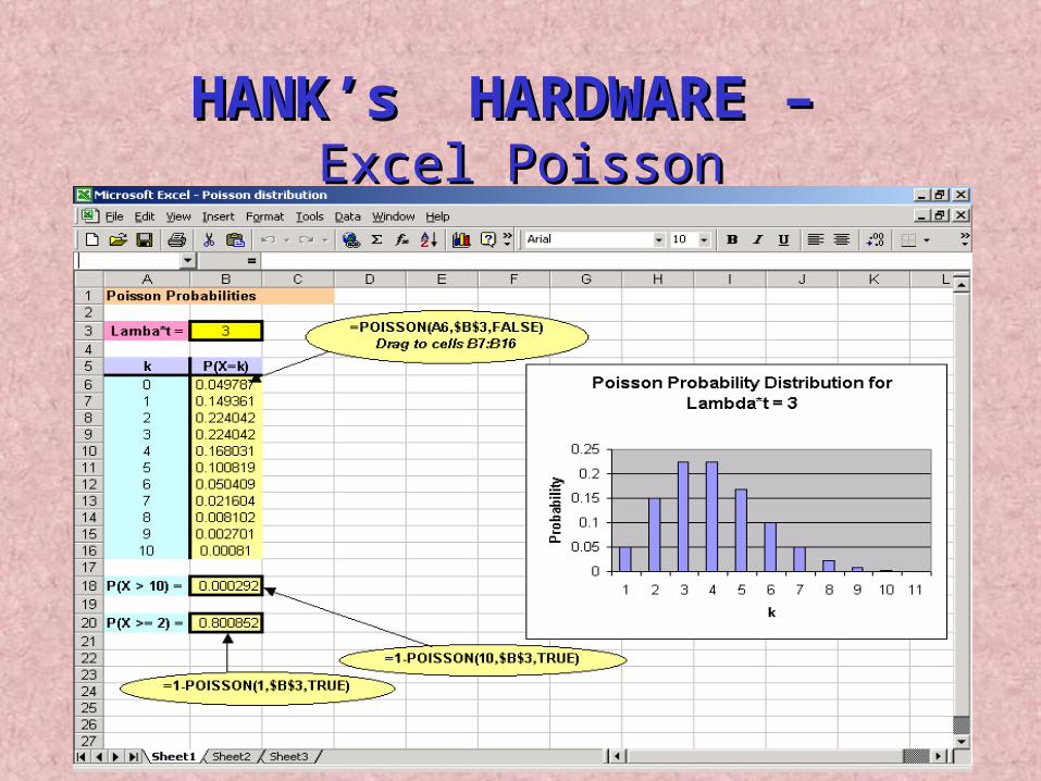
HANK’s HARDWARE – HANK’s HARDWARE – Excel PoissonExcel Poisson

12
• Factors that influence the modeling of queues
– Line configuration
– Jockeying
– Balking
The Waiting Line CharacteristicsThe Waiting Line Characteristics
– Priority
– Tandem Queues
– Homogeneity
13
• A single service queue.• Multiple service queue with single waiting line.• Multiple service queue with multiple waiting
lines.• Tandem queue (multistage service system).
Line ConfigurationLine Configuration
14
• Jockeying occurs when customers switch lines once they perceived that another line is moving faster.
• Balking occurs if customers avoid joining the line when they perceive the line to be too long.
Jockeying and BalkingJockeying and Balking
15
• These rules select the next customer for service.• There are several commonly used rules:
– First come first served (FCFS).– Last come first served (LCFS).– Estimated service time.– Random selection of customers for service.
Priority RulesPriority Rules
16
Tandem QueuesTandem Queues
• These are multi-server systems. • A customer needs to visit several service
stations (usually in a distinct order) to complete the service process.
• Examples– Patients in an emergency room.– Passengers prepare for the next flight.
17
• A homogeneous customer population is one in which customers require essentially the same type of service.
• A non-homogeneous customer population is one in which customers can be categorized according to: – Different arrival patterns– Different service treatments.
HomogeneityHomogeneity
18
• In most business situations, service time varies widely among customers.
• When service time varies, it is treated as a random variable.
• The exponential probability distribution is used sometimes to model customer service time.
The Service ProcessThe Service Process
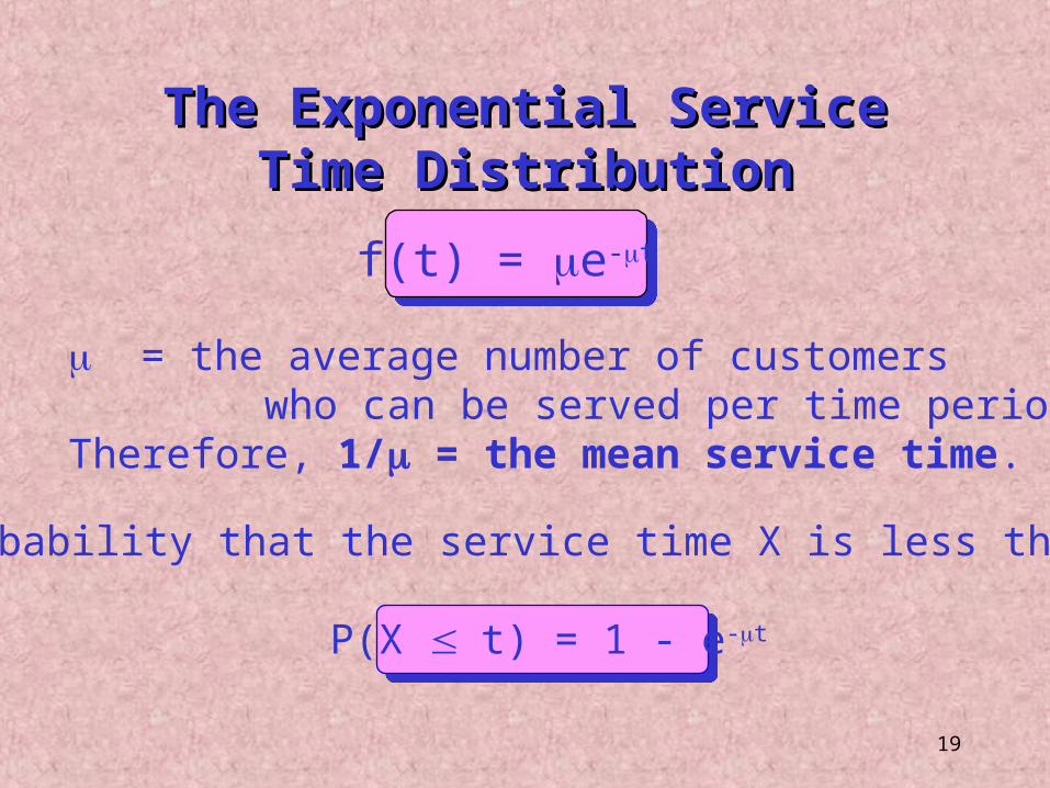
19
f(t) = e-t
= the average number of customers who can be served per time period.Therefore, 1/ = the mean service time.
The probability that the service time X is less than some “t.”
P(X t) = 1 - e-t
The Exponential Service Time DistributionThe Exponential Service Time Distribution
20
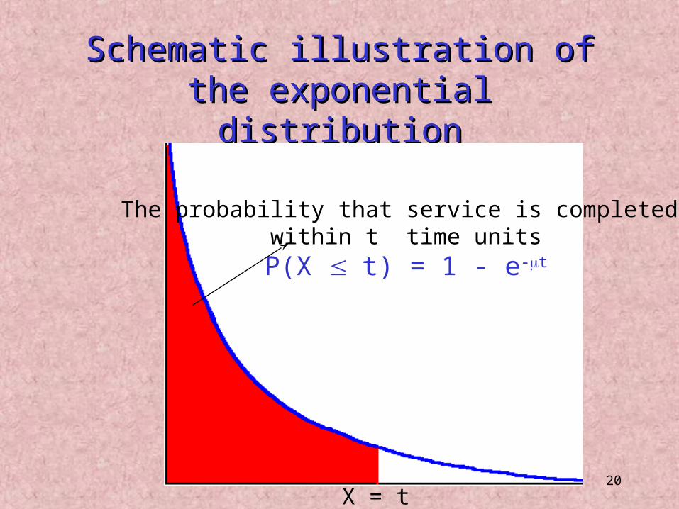
Schematic illustration of the exponential Schematic illustration of the exponential distributiondistribution
The probability that service is completed within t time units
P(X t) = 1 - e-t
X = t
21
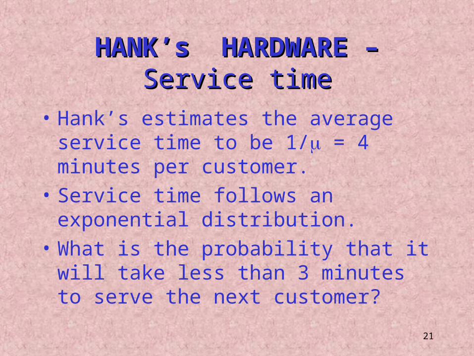
HANK’s HARDWARE – HANK’s HARDWARE – Service timeService time
• Hank’s estimates the average service time to be 1/ = 4 minutes per customer.
• Service time follows an exponential distribution.• What is the probability that it will take less than 3
minutes to serve the next customer?
22
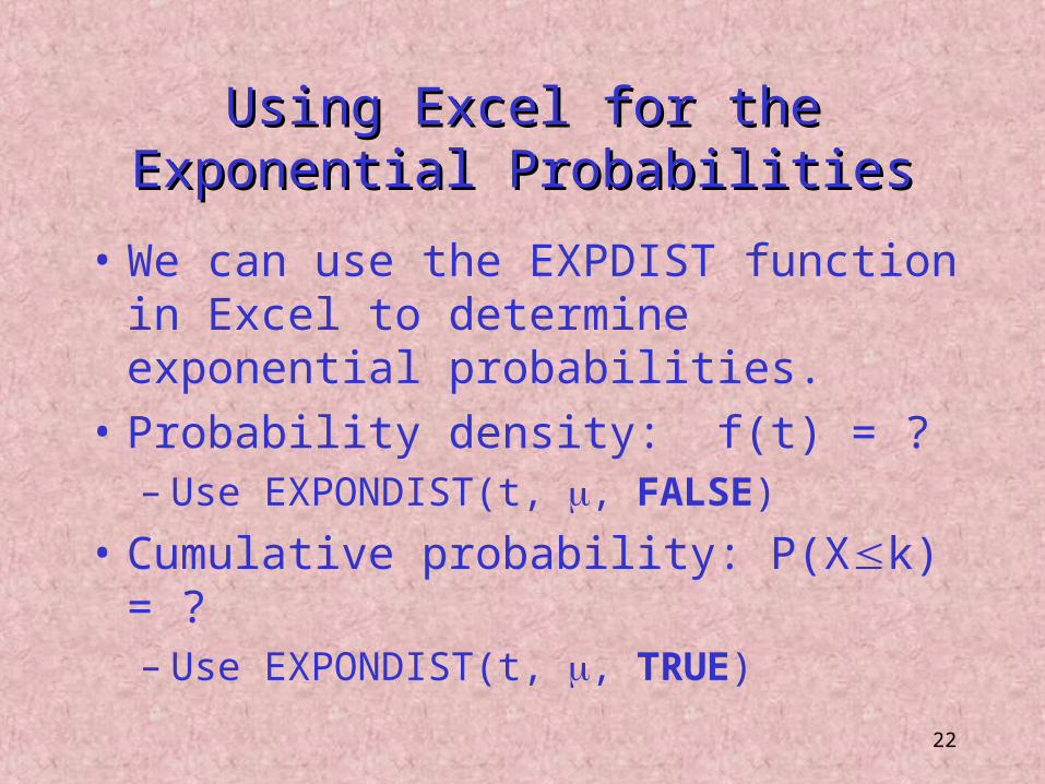
• We can use the EXPDIST function in Excel to determine exponential probabilities.
• Probability density: f(t) = ?– Use EXPONDIST(t, , FALSE)
• Cumulative probability: P(Xk) = ?– Use EXPONDIST(t, , TRUE)
Using Excel for the Exponential ProbabilitiesUsing Excel for the Exponential Probabilities
23
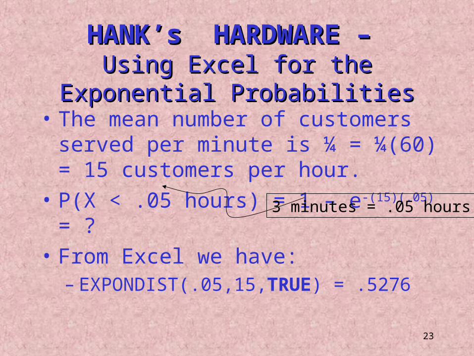
• The mean number of customers served per minute is ¼ = ¼(60) = 15 customers per hour.
• P(X < .05 hours) = 1 – e-(15)(.05) = ?• From Excel we have:
– EXPONDIST(.05,15,TRUE) = .5276
HANK’s HARDWARE – HANK’s HARDWARE – Using Excel for the Exponential ProbabilitiesUsing Excel for the Exponential Probabilities
3 minutes = .05 hours
24
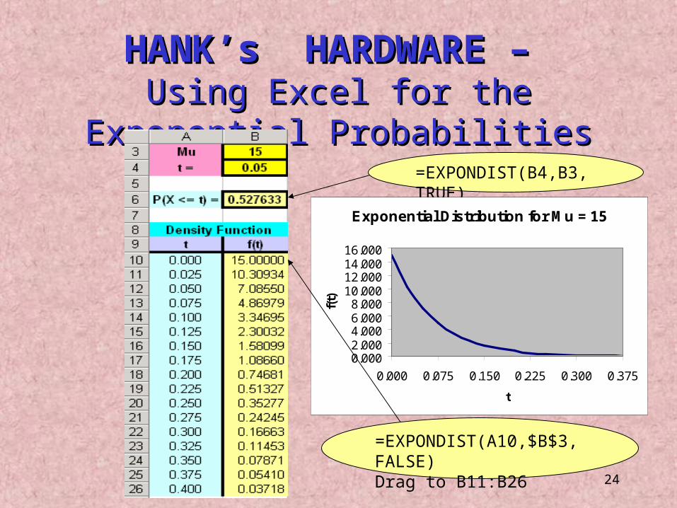
HANK’s HARDWARE – HANK’s HARDWARE – Using Excel for the Exponential ProbabilitiesUsing Excel for the Exponential Probabilities
=EXPONDIST(B4,B3,TRUE)
Exponential Distribution for Mu = 15
0.0002.0004.0006.0008.000
10.00012.00014.00016.000
0.000 0.075 0.150 0.225 0.300 0.375
t
f(t)
=EXPONDIST(A10,$B$3,FALSE)Drag to B11:B26
25
• The memoryless property.– No additional information about the time left for the completion of a
service, is gained by recording the time elapsed since the service started.
– For Hank’s, the probability of completing a service within the next 3 minutes is (0.52763) independent of how long the customer has been served already.
• The Exponential and the Poisson distributions are related to one another.
– If customer arrivals follow a Poisson distribution with mean rate , their interarrival times are exponentially distributed with mean time 1/
The Exponential Distribution -The Exponential Distribution - CharacteristicsCharacteristics
26
9.3 Performance Measures of 9.3 Performance Measures of Queuing System Queuing System
• Performance can be measured by focusing on:– Customers in queue.
– Customers in the system.
• Performance is measured for a system in steady state.
27
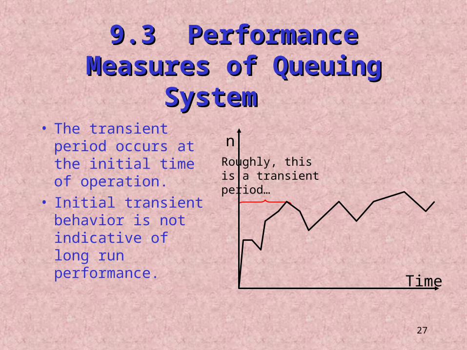
Roughly, this is a transient period…
n
Time
9.3 Performance Measures of 9.3 Performance Measures of Queuing System Queuing System
• The transient period occurs at the initial time of operation.
• Initial transient behavior is not indicative of long run performance.
28
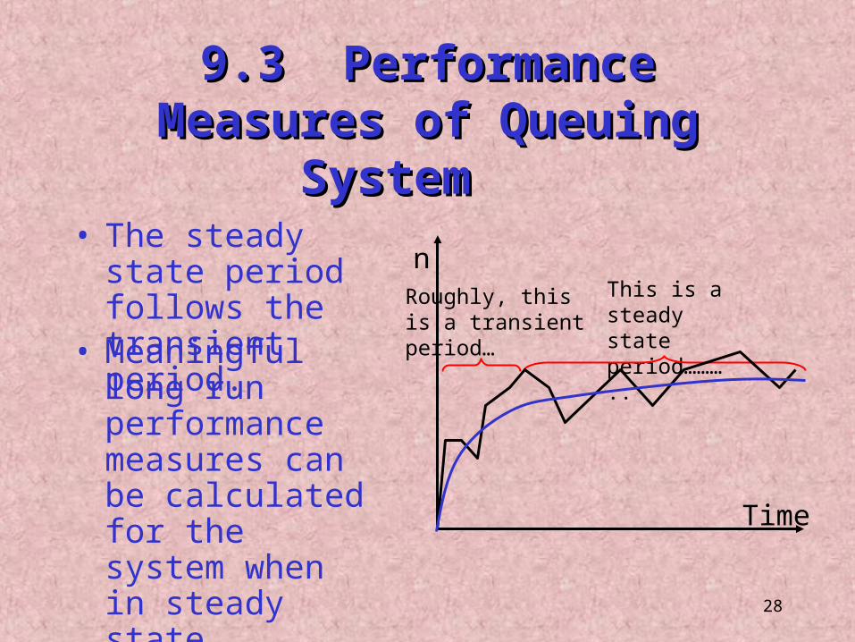
This is a steady state period………..
n
Time
9.3 Performance Measures of 9.3 Performance Measures of Queuing System Queuing System
• The steady state period follows the transient period.
• Meaningful long run performance measures can be calculated for the system when in steady state.
Roughly, this is a transient period…
29
kEach with
service rate of
kEach with
service rate of
…For k servers
with service rates
…For k servers
with service rates
For one server
For one server
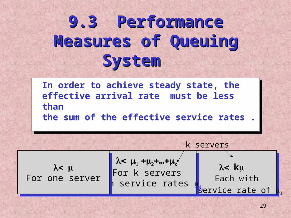
In order to achieve steady state, theeffective arrival rate must be less than the sum of the effective service rates .
In order to achieve steady state, theeffective arrival rate must be less than the sum of the effective service rates .
9.3 Performance Measures of 9.3 Performance Measures of Queuing System Queuing System
k servers
30
Example :Example :
• Suppose – customers arrrive at the rate of =20 per hour– there are 3 servers, each serving an average of 4
customers per hour • You will
– serve an average of 12 customers per hour– add 8 customers each hour to your waiting line
31
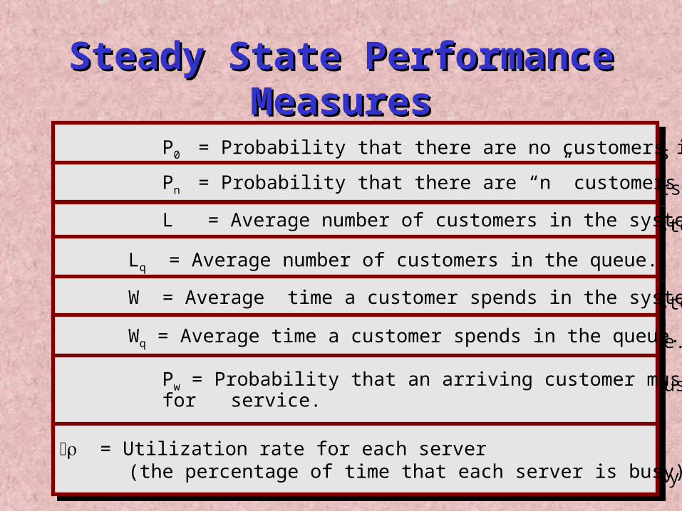
P0 = Probability that there are no customers in the system.P0 = Probability that there are no customers in the system.
Pn = Probability that there are “n” customers in the system.Pn = Probability that there are “n” customers in the system.
L = Average number of customers in the system.L = Average number of customers in the system.
Lq = Average number of customers in the queue.Lq = Average number of customers in the queue.
W = Average time a customer spends in the system.W = Average time a customer spends in the system.
Wq = Average time a customer spends in the queue.Wq = Average time a customer spends in the queue.
Pw = Probability that an arriving customer must wait for service.
Pw = Probability that an arriving customer must wait for service.
= Utilization rate for each server (the percentage of time that each server is busy).
= Utilization rate for each server (the percentage of time that each server is busy).
Steady State Performance MeasuresSteady State Performance Measures
32
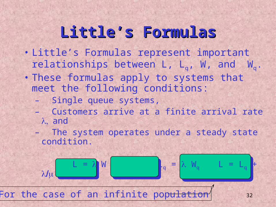
• Little’s Formulas represent important relationships between L, Lq, W, and Wq.
• These formulas apply to systems that meet the following conditions:– Single queue systems,– Customers arrive at a finite arrival rate and– The system operates under a steady state condition.
L =W Lq = Wq L = Lq +
Little’s FormulasLittle’s Formulas
For the case of an infinite population
33
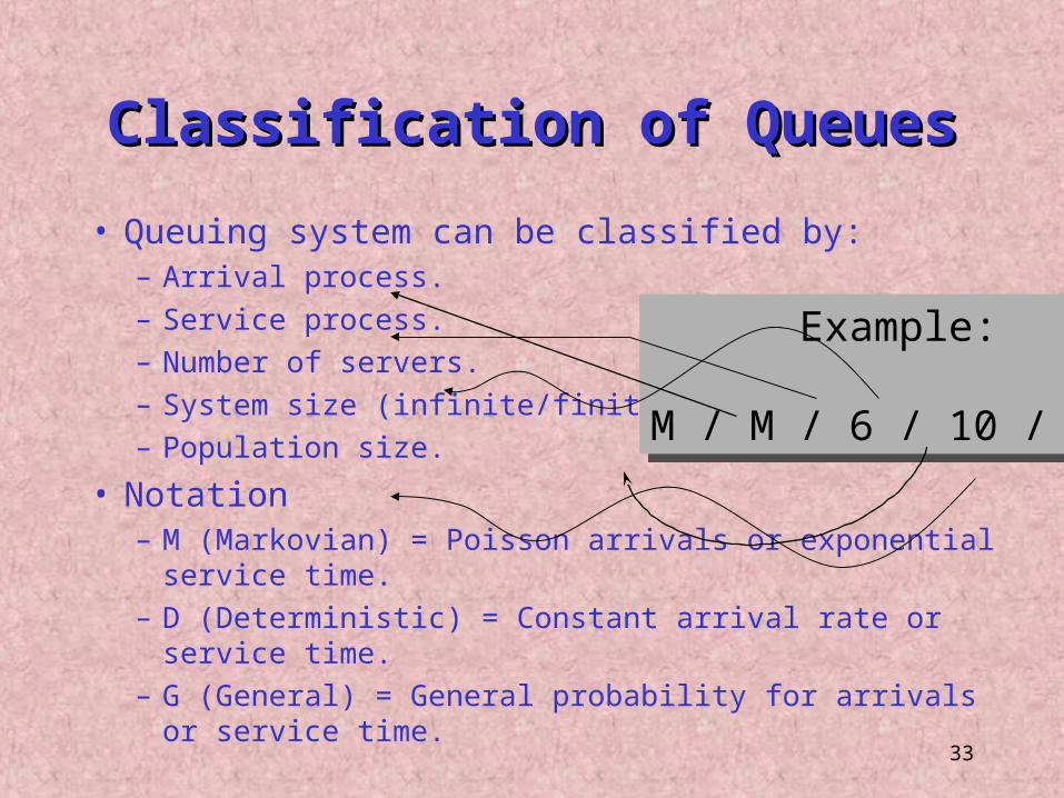
• Queuing system can be classified by:– Arrival process.– Service process.– Number of servers.– System size (infinite/finite waiting line).– Population size.
• Notation– M (Markovian) = Poisson arrivals or exponential service time.– D (Deterministic) = Constant arrival rate or service time.– G (General) = General probability for arrivals or service time.
Example:
M / M / 6 / 10 / 20
Example:
M / M / 6 / 10 / 20
Classification of QueuesClassification of Queues
34
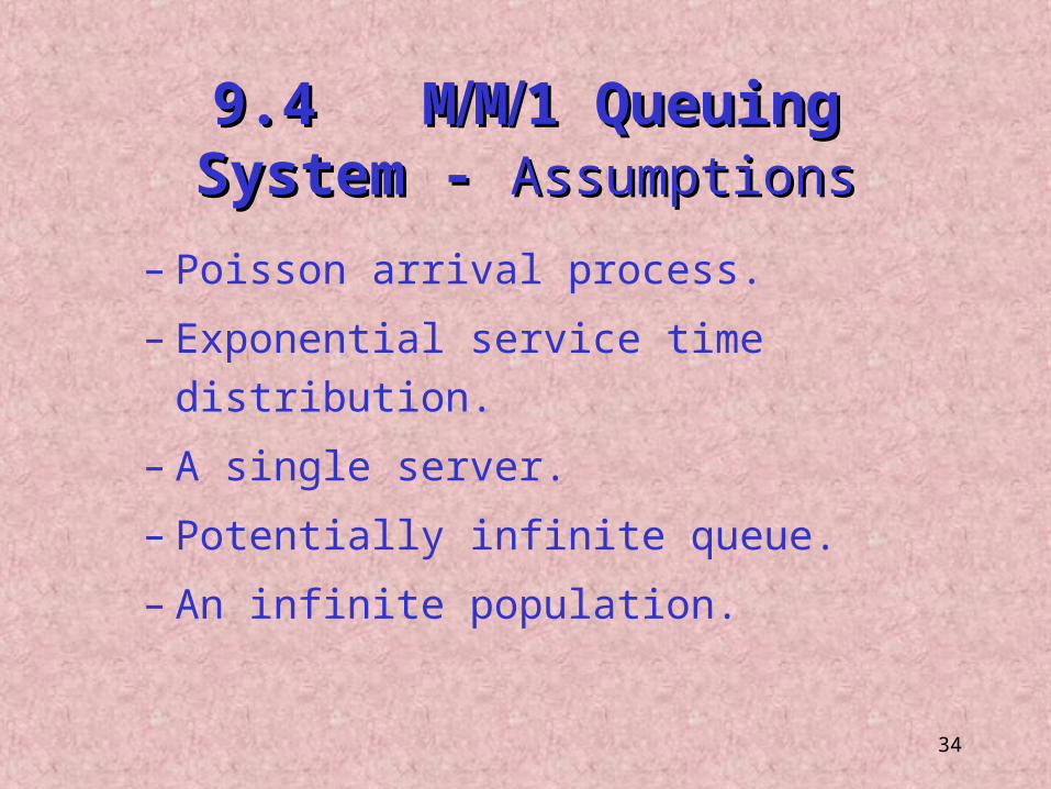
9.4 M9.4 MMM1 Queuing System - 1 Queuing System - AssumptionsAssumptions
– Poisson arrival process.
– Exponential service time distribution.
– A single server.
– Potentially infinite queue.
– An infinite population.
35
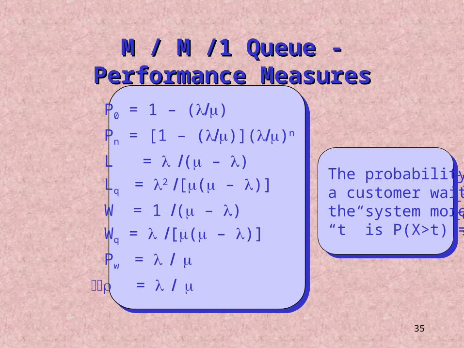
The probability thata customer waits in the system more than “t” is P(X>t) = e-( - )t
The probability thata customer waits in the system more than “t” is P(X>t) = e-( - )t
P0 = 1 – ()
Pn = [1 – ()]()n
L = ( – )Lq = 2 [( – )]
W = 1 ( – )Wq = [( – )]
Pw =
=
M / M /1 Queue - Performance MeasuresM / M /1 Queue - Performance Measures
36
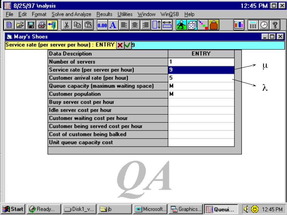
MARY’s SHOESMARY’s SHOES
• Customers arrive at Mary’s Shoes every 12 minutes on the average, according to a Poisson process.
• Service time is exponentially distributed with an average of 8 minutes per customer.
• Management is interested in determining the performance measures for this service system.
37
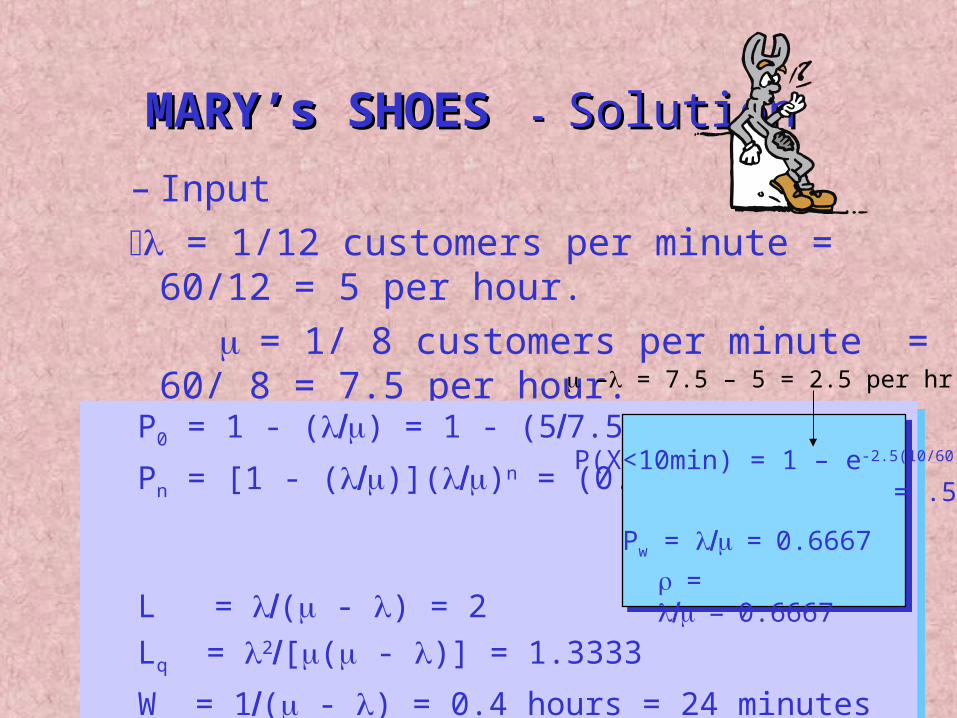
MARY’s SHOESMARY’s SHOES - - SolutionSolution– Input = 1/12 customers per minute = 60/12 = 5 per hour. = 1/ 8 customers per minute = 60/ 8 = 7.5 per hour.
– Performance Calculations
P0 = 1 - () = 1 - (57.5) = 0.3333
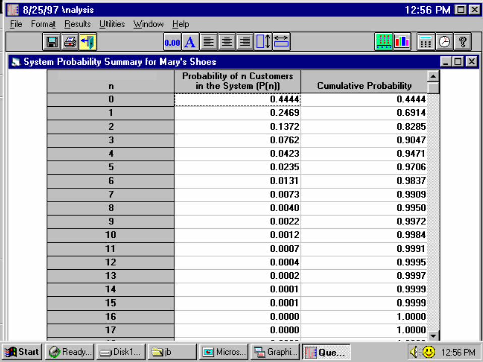
Pn = [1 - ()]()n = (0.3333)(0.6667)n L = ( - ) = 2Lq = 2[( - )] = 1.3333
W = 1( - ) = 0.4 hours = 24 minutesWq = ( - )] = 0.26667 hours = 16 minutes
P0 = 1 - () = 1 - (57.5) = 0.3333
Pn = [1 - ()]()n = (0.3333)(0.6667)n L = ( - ) = 2Lq = 2[( - )] = 1.3333
W = 1( - ) = 0.4 hours = 24 minutesWq = ( - )] = 0.26667 hours = 16 minutes
Pw = =0.6667= =0.6667
P(X<10min) = 1 – e-2.5(10/60)
= .565
– = 7.5 – 5 = 2.5 per hr.
38
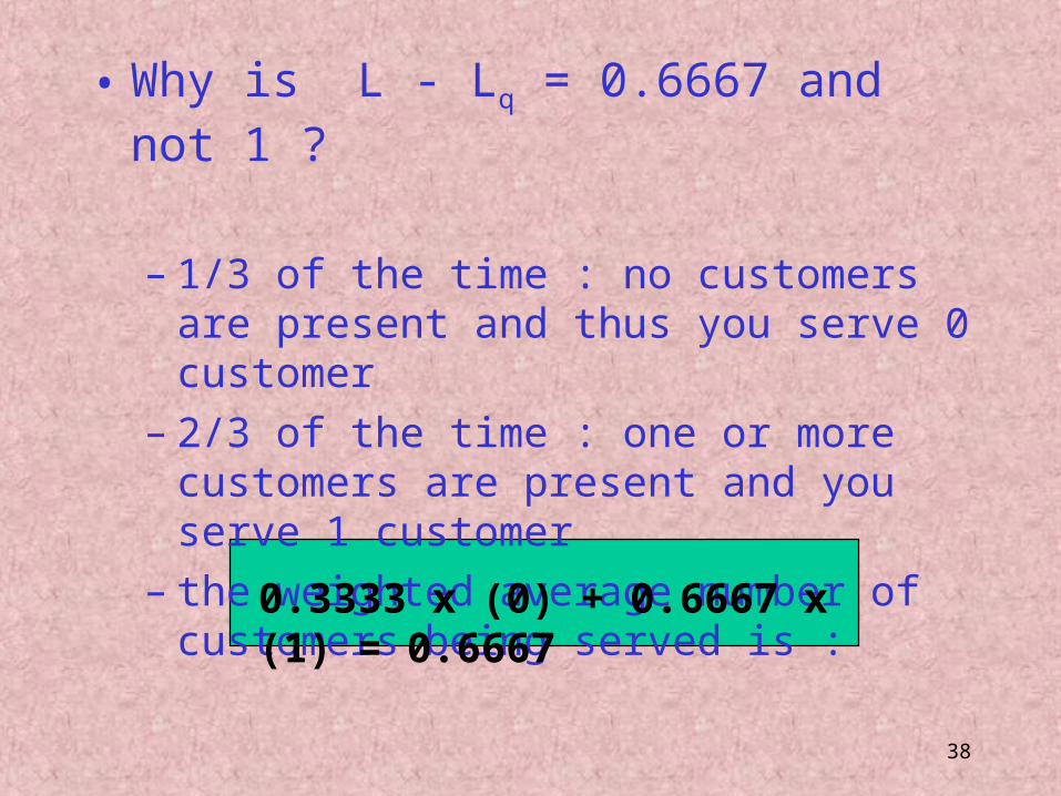
• Why is L - Lq = 0.6667 and not 1 ?
– 1/3 of the time : no customers are present and thus you serve 0 customer
– 2/3 of the time : one or more customers are present and you serve 1 customer
– the weighted average number of customers being served is :
0.3333 x (0) + 0.6667 x (1) = 0.6667
39
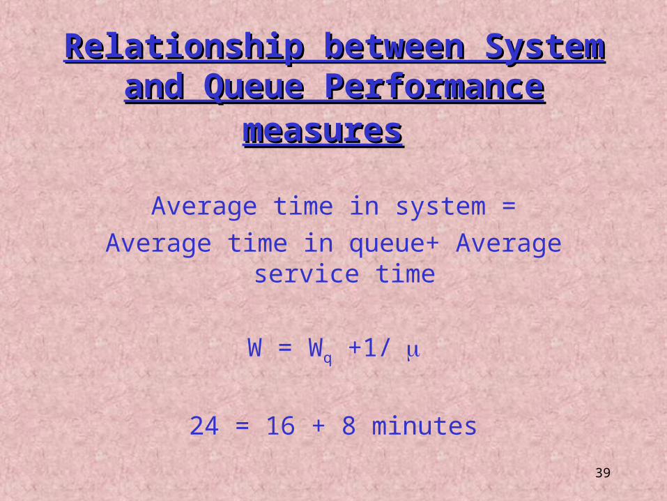
Relationship between System and Queue Relationship between System and Queue Performance measuresPerformance measures
Average time in system =Average time in queue+ Average service time
W = Wq +1/
24 = 16 + 8 minutes
40
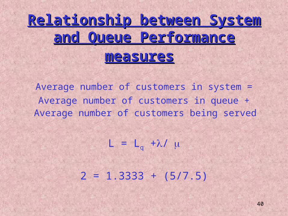
Relationship between System and Queue Relationship between System and Queue Performance measuresPerformance measures
Average number of customers in system =Average number of customers in queue + Average number of
customers being served
L = Lq +/
2 = 1.3333 + (5/7.5)
41
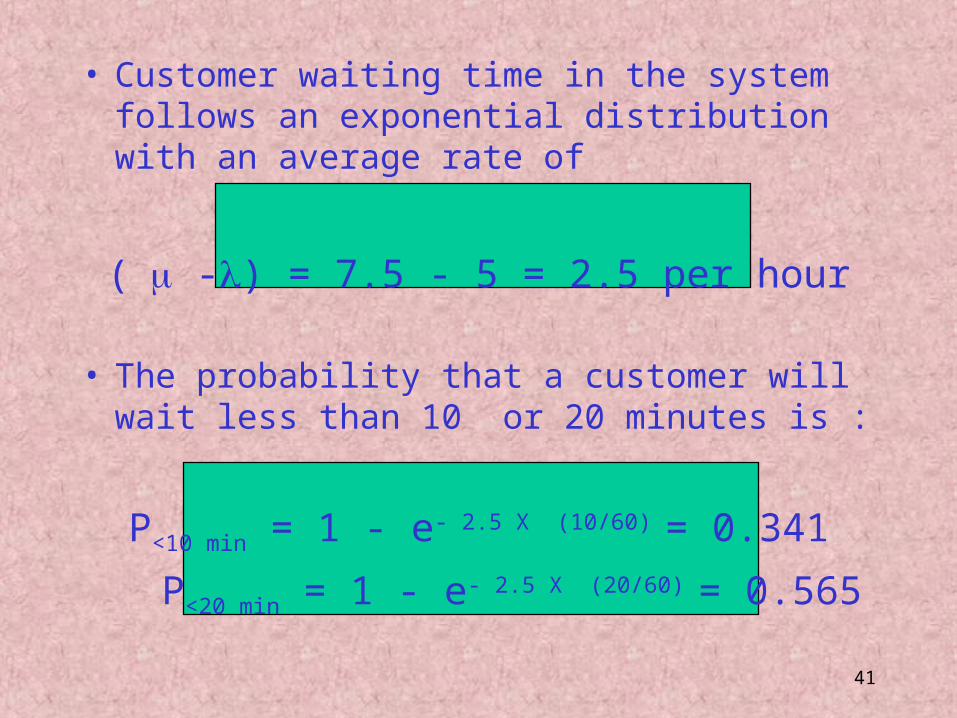
• Customer waiting time in the system follows an exponential distribution with an average rate of
( -) = 7.5 - 5 = 2.5 per hour
• The probability that a customer will wait less than 10 or 20 minutes is :
P<10 min = 1 - e- 2.5 X (10/60) = 0.341
P<20 min = 1 - e- 2.5 X (20/60) = 0.565
42
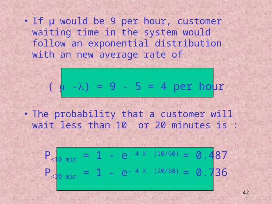
• If µ would be 9 per hour, customer waiting time in the system would follow an exponential distribution with an new average rate of
( -) = 9 - 5 = 4 per hour
• The probability that a customer will wait less than 10 or 20 minutes is :
P<10 min = 1 - e- 4 X (10/60) = 0.487
P<20 min = 1 - e- 4 X (20/60) = 0.736
43
WINQSB Input ScreenWINQSB Input Screen
44
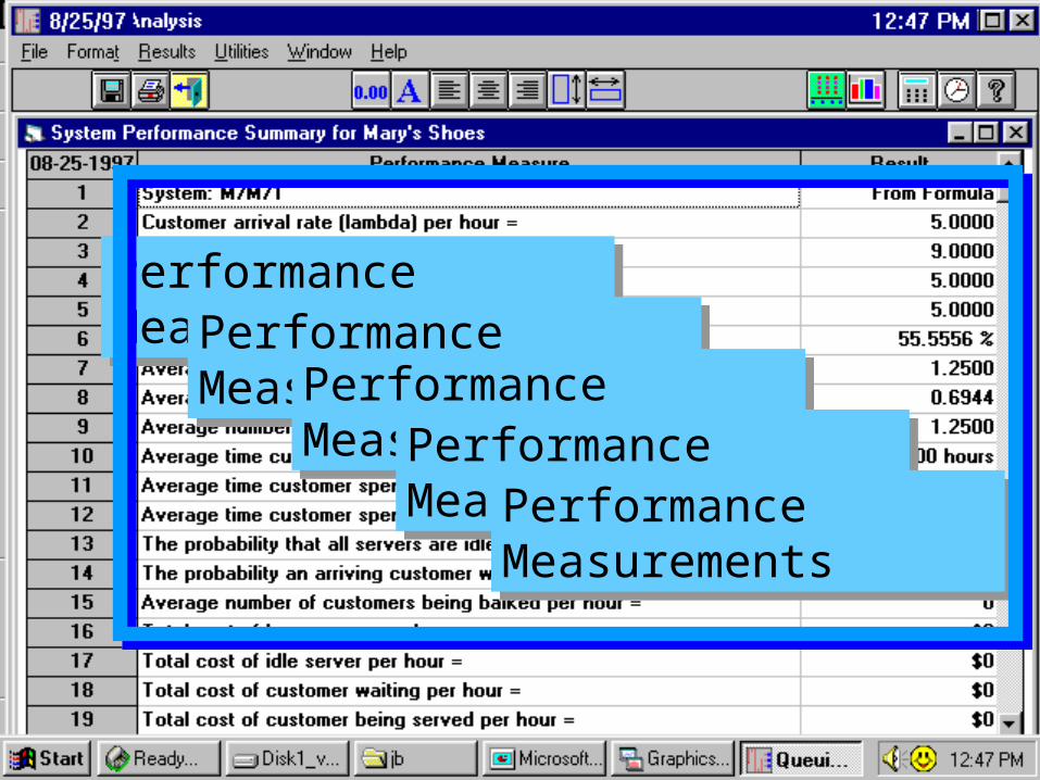
Performance MeasurementsPerformance MeasurementsPerformance MeasurementsPerformance Measurements
Performance MeasurementsPerformance MeasurementsPerformance MeasurementsPerformance Measurements
Performance MeasurementsPerformance Measurements
45
46
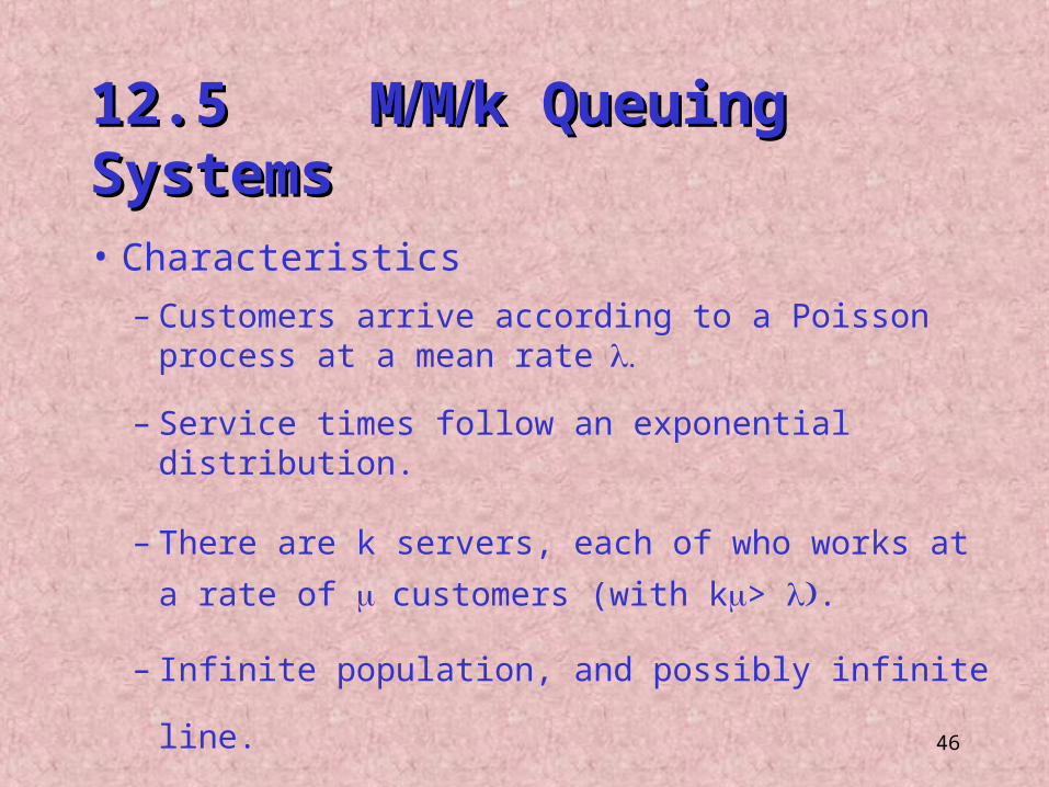
12.5 M12.5 MMMk Queuing Systemsk Queuing Systems
• Characteristics– Customers arrive according to a Poisson process at a
mean rate
– Service times follow an exponential distribution.
– There are k servers, each of who works at a rate of
customers (with k> .
– Infinite population, and possibly infinite line.
47
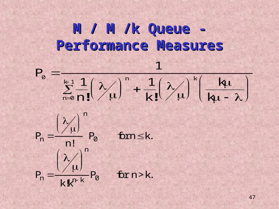
P
n kk
k
n k
n
k0
0
1
11 1
! !
Pn
P
k kP
n
n
n
n k
!
!
0
0
for n k.
P for n > k.n
M / M /k Queue - Performance MeasuresM / M /k Queue - Performance Measures
48
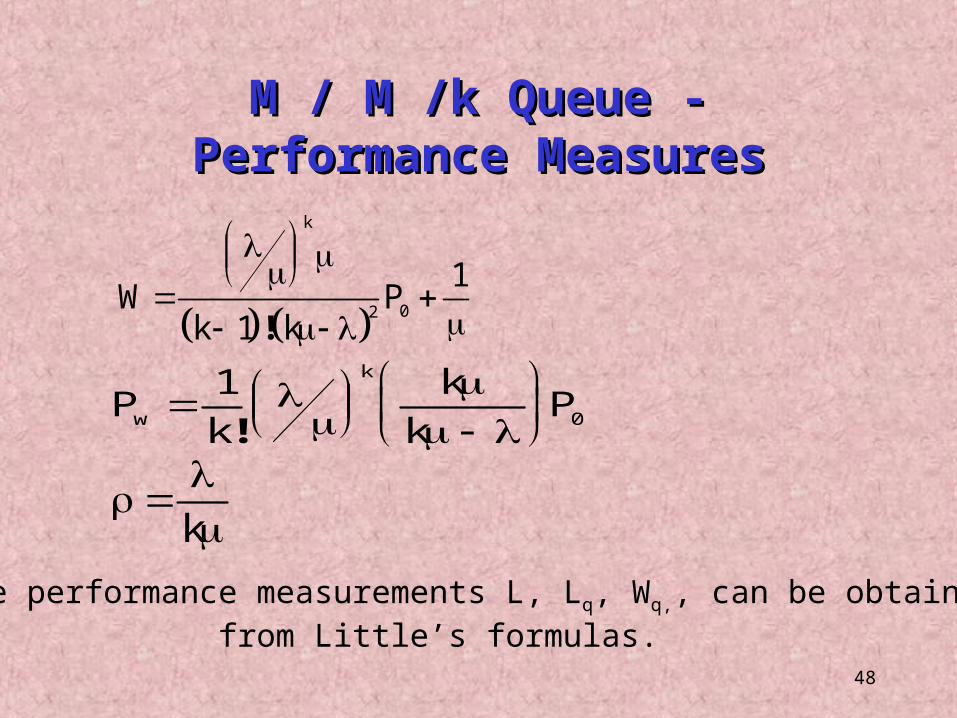
W
k kP
k
1
12 0
!
The performance measurements L, Lq, Wq,, can be obtained from Little’s formulas.
Pk
kk
Pw
k
10!
k
M / M /k Queue - Performance MeasuresM / M /k Queue - Performance Measures
49
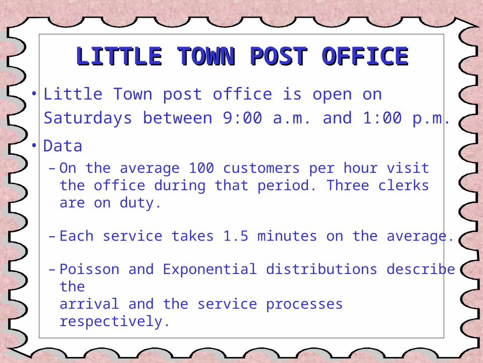
LITTLE TOWN POST OFFICELITTLE TOWN POST OFFICE
• Little Town post office is open on Saturdays between 9:00 a.m. and 1:00 p.m.
• Data– On the average 100 customers per hour visit the office
during that period. Three clerks are on duty.
– Each service takes 1.5 minutes on the average.
– Poisson and Exponential distributions describe the arrival and the service processes respectively.
50
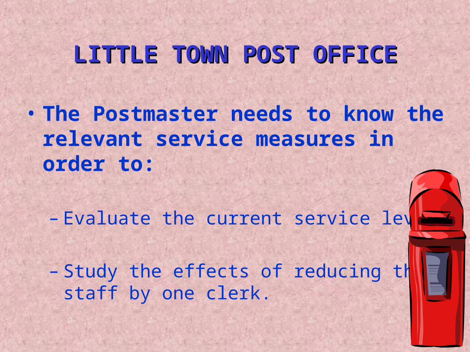
LITTLE TOWN POST OFFICELITTLE TOWN POST OFFICE
• The Postmaster needs to know the relevant service measures in order to:
– Evaluate the current service level.
– Study the effects of reducing the staff by one clerk.
51
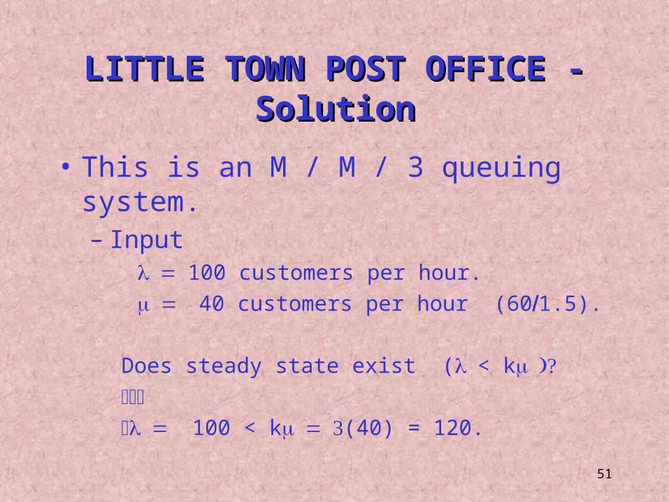
• This is an M / M / 3 queuing system.– Input
100 customers per hour.40 customers per hour (601.5).
Does steady state exist (< k 100 < k(40) = 120.
LITTLE TOWN POST OFFICE - SolutionLITTLE TOWN POST OFFICE - Solution
52
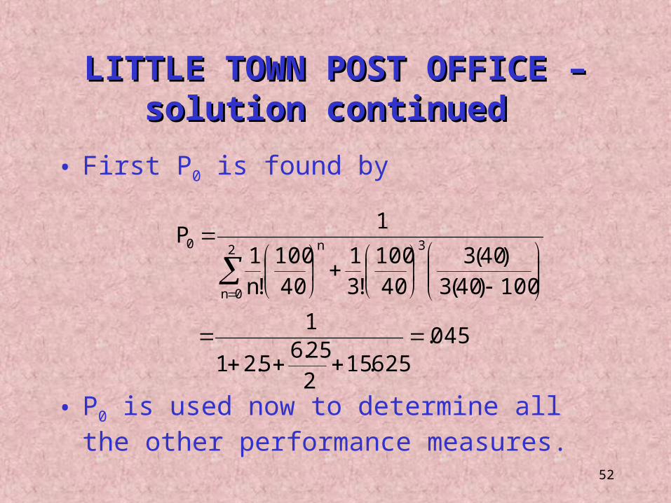
LITTLE TOWN POST OFFICE – solution LITTLE TOWN POST OFFICE – solution continued continued
• First P0 is found by
045.625.15
225.6
5.21
1
100)40(3)40(3
40100
!31
40100
!n1
1P
2
0n
3n0
• P0 is used now to determine all the other performance measures.
53
LITTLE TOWN POST OFFICE –LITTLE TOWN POST OFFICE –
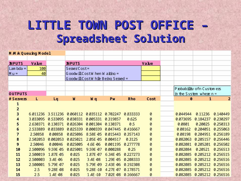
Spreadsheet SolutionSpreadsheet SolutionM/M/k Queuing Model
INPUTS Value INPUTS ValueLambda = 100Mu = 40
OUTPUTS# Servers L Lq W Wq Pw Rho Cost 0 1 2
123 6.011236 3.511236 0.060112 0.035112 0.702247 0.833333 0 0.044944 0.11236 0.1404494 3.033095 0.533095 0.030331 0.005331 0.319857 0.625 0 0.073695 0.184237 0.2302975 2.630371 0.130371 0.026304 0.001304 0.130371 0.5 0 0.0801 0.20025 0.2503136 2.533889 0.033889 0.025339 0.000339 0.047445 0.416667 0 0.08162 0.204051 0.2550637 2.50858 0.00858 0.025086 8.58E-05 0.015443 0.357143 0 0.08198 0.204951 0.2561898 2.502053 0.002053 0.025021 2.05E-05 0.004517 0.3125 0 0.082063 0.205157 0.2564469 2.50046 0.00046 0.025005 4.6E-06 0.001195 0.277778 0 0.082081 0.205201 0.25650210 2.500096 9.59E-05 0.025001 9.59E-07 0.000288 0.25 0 0.082084 0.20521 0.25651311 2.500019 1.87E-05 0.025 1.87E-07 6.34E-05 0.227273 0 0.082085 0.205212 0.25651512 2.500003 3.4E-06 0.025 3.4E-08 1.29E-05 0.208333 0 0.082085 0.205212 0.25651613 2.500001 5.79E-07 0.025 5.79E-09 2.43E-06 0.192308 0 0.082085 0.205212 0.25651614 2.5 9.28E-08 0.025 9.28E-10 4.27E-07 0.178571 0 0.082085 0.205212 0.25651615 2.5 1.4E-08 0.025 1.4E-10 7.02E-08 0.166667 0 0.082085 0.205212 0.256516
in the System where n =Probabiility of n Customers
Server Cost =Goodwill Cost When Waiting =Goodwill Cost While Being Served =
54
9.6 M9.6 MGG1 Queuing System1 Queuing System
• Assumptions– Customers arrive according to a Poisson process with a
mean rate– Service time has a general distribution with mean rate
– One server.
– Infinite population, and possibly infinite line.
55
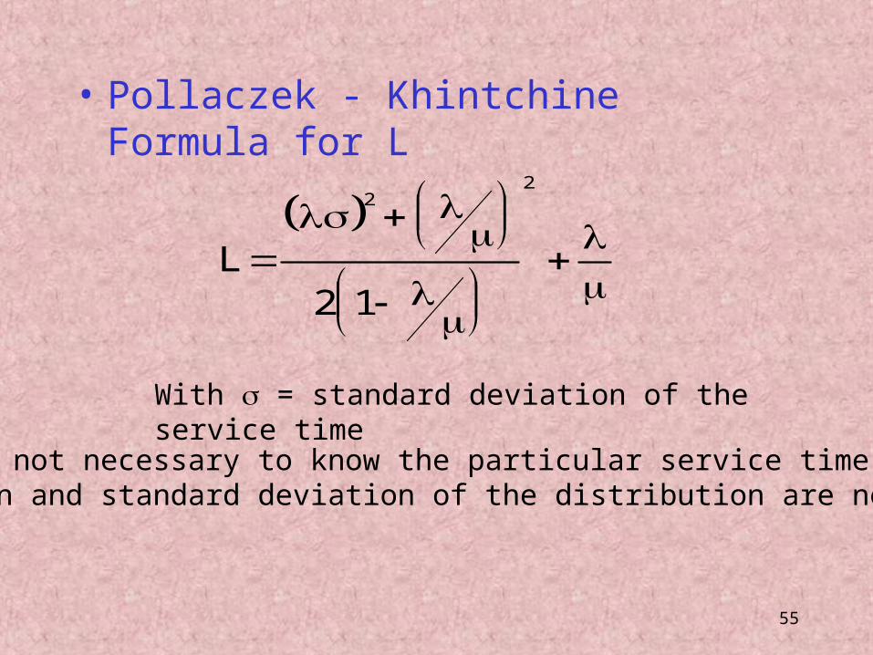
• Pollaczek - Khintchine Formula for L
L
22
2 1
Note: It is not necessary to know the particular service time distribution.Only the mean and standard deviation of the distribution are needed.
With = standard deviation of the service time
56
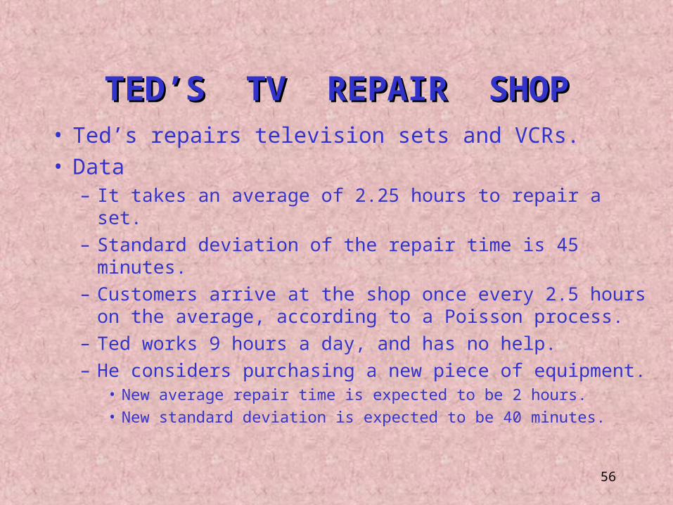
• Ted’s repairs television sets and VCRs.• Data
– It takes an average of 2.25 hours to repair a set.– Standard deviation of the repair time is 45 minutes.– Customers arrive at the shop once every 2.5 hours on the
average, according to a Poisson process.– Ted works 9 hours a day, and has no help.– He considers purchasing a new piece of equipment.
• New average repair time is expected to be 2 hours.• New standard deviation is expected to be 40 minutes.
TED’S TV REPAIR SHOPTED’S TV REPAIR SHOP
57
Ted wants to know the effects of using the new equipment on –
1. The average number of sets waiting for repair;
2. The average time a customer has to wait to get his repaired set.
TED’S TV REPAIR SHOPTED’S TV REPAIR SHOP
58
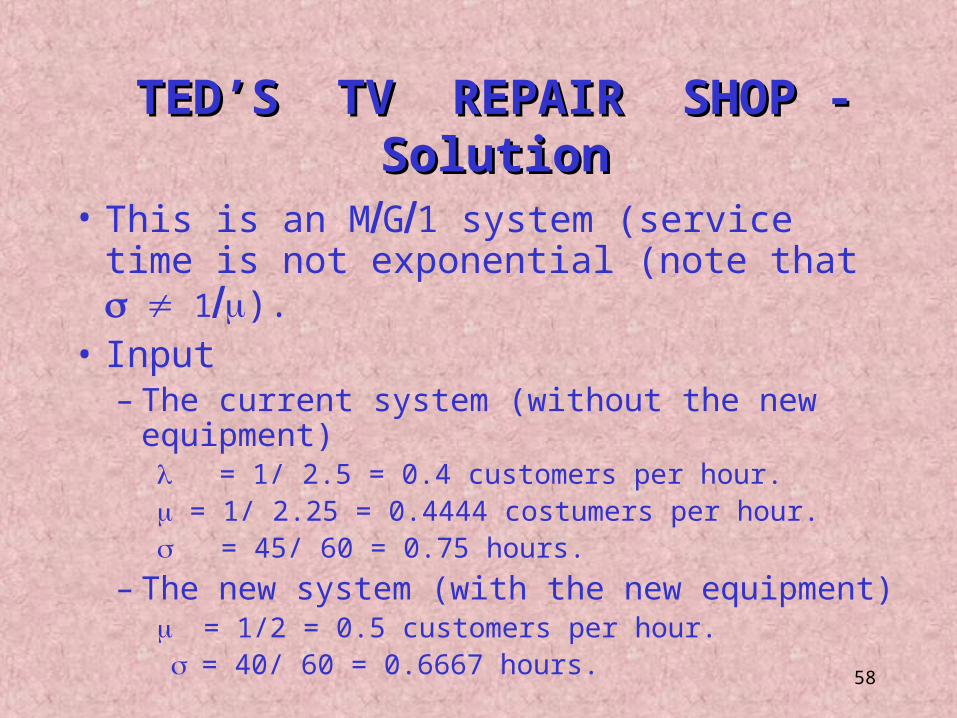
• This is an MG1 system (service time is not exponential (note that 1).
• Input– The current system (without the new equipment)
= 1/ 2.5 = 0.4 customers per hour. = 1/ 2.25 = 0.4444 costumers per hour. = 45/ 60 = 0.75 hours.
– The new system (with the new equipment) = 1/2 = 0.5 customers per hour.= 40/ 60 = 0.6667 hours.
TED’S TV REPAIR SHOP - SolutionTED’S TV REPAIR SHOP - Solution
59
9.7 M / M / k / F Queuing System9.7 M / M / k / F Queuing System
• Many times queuing systems have designs that limit their line size.
• When the potential queue is large, an infinite queue model gives accurate results, even though the queue might be limited.
• When the potential queue is small, the limited line must be accounted for in the model.
60
• Poisson arrival process at mean rate
• k servers, each having an exponential service time with mean rate
• Maximum number of customers that can be present in the system at any one time is “F”.
• Customers are blocked (and never return) if the system is full.
Characteristics of MCharacteristics of MMMkkF Queuing SystemF Queuing System
61
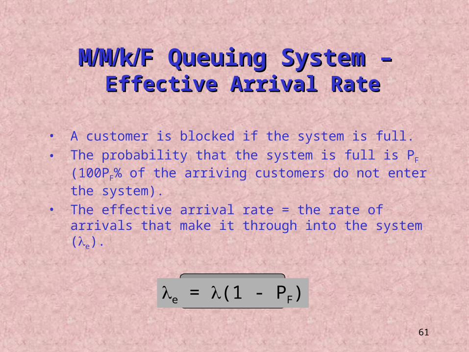
• A customer is blocked if the system is full.• The probability that the system is full is PF (100PF% of
the arriving customers do not enter the system).• The effective arrival rate = the rate of arrivals that
make it through into the system (e).
e = (1 - PF)
MMMMkkF Queuing System – F Queuing System – Effective Arrival RateEffective Arrival Rate
62
RYAN ROOFING COMPANYRYAN ROOFING COMPANY
• Ryan gets most of its business from customers who call and order service.– When a telephone line is available but the secretary
is busy serving a customer, a new calling customer is willing to wait until the secretary becomes available.
– When all the lines are busy, a new calling customer gets a busy signal and calls a competitor.
63
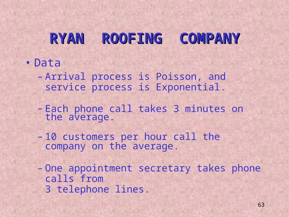
• Data– Arrival process is Poisson, and service process is
Exponential.
– Each phone call takes 3 minutes on the average.
– 10 customers per hour call the company on the average.
– One appointment secretary takes phone calls from 3 telephone lines.
RYAN ROOFING COMPANYRYAN ROOFING COMPANY
64
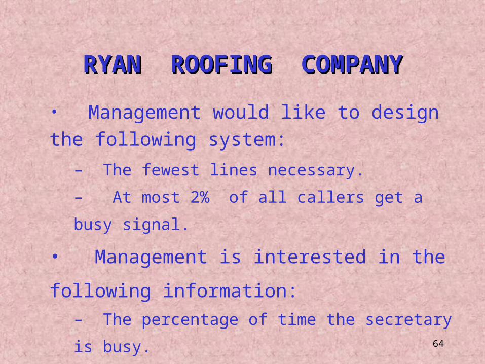
• Management would like to design the following system:– The fewest lines necessary.
– At most 2% of all callers get a busy signal.
• Management is interested in the following information:– The percentage of time the secretary is busy.
– The average number of customers kept on hold.
– The average time a customer is kept on hold.
– The actual percentage of callers who encounter a busy signal.
RYAN ROOFING COMPANYRYAN ROOFING COMPANY
65
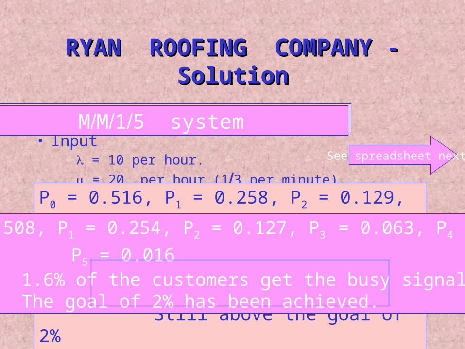
• This is an MM13 system• Input
= 10 per hour. = 20 per hour (13 per minute).
• Excel spreadsheet gives: P0 = 0.533, P1 = 0.133, P3 = 0.06
6.7% of the customers get a busy signal.
This is above the goal of 2%.
P0 = 0.516, P1 = 0.258, P2 = 0.129, P3 = 0.065, P4 = 0.032
3.2% of the customers get the busy signal Still above the goal of 2%
RYAN ROOFING COMPANY - SolutionRYAN ROOFING COMPANY - Solution
MM14 system MM15 system
P0 = 0.508, P1 = 0.254, P2 = 0.127, P3 = 0.063, P4 = 0.032P5 = 0.016
1.6% of the customers get the busy signal The goal of 2% has been achieved.
See spreadsheet next
66
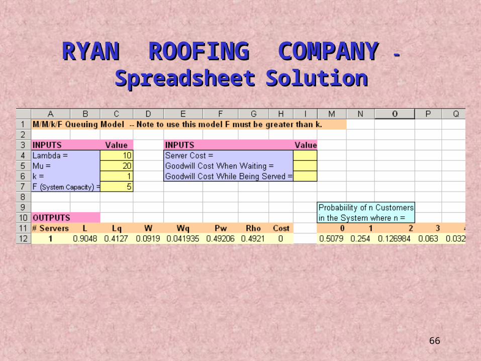
RYAN ROOFING COMPANYRYAN ROOFING COMPANY - -
SpreadsheetSpreadsheet SolutionSolution
67
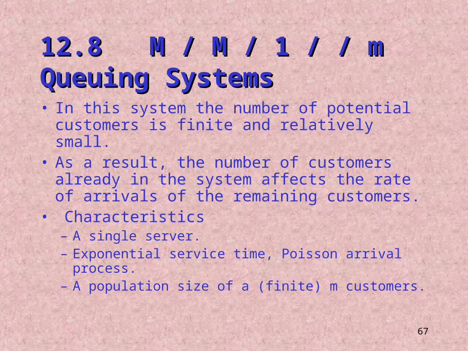
12.8 M / M / 1 / / m Queuing Systems12.8 M / M / 1 / / m Queuing Systems
• In this system the number of potential customers is finite and relatively small.
• As a result, the number of customers already in the system affects the rate of arrivals of the remaining customers.
• Characteristics– A single server.– Exponential service time, Poisson arrival process.– A population size of a (finite) m customers.

68
PACESETTER HOMESPACESETTER HOMES
• Pacesetter Homes runs four different development projects.• Data
– At each site running a project is interrupted once every 20 working days on the average.
– The V.P. for construction handles each stoppage.• How long on the average a site is non-operational?
– If it takes 2 days on the average to restart a project’s progress (the V.P. is using the current car).
– If it takes 1.875 days on the average to restart a project’s progress (the V.P. is using a new car)
69
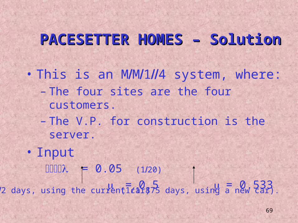
PACESETTER HOMES – SolutionPACESETTER HOMES – Solution
• This is an MM14 system, where:– The four sites are the four customers.– The V.P. for construction is the server.
• Input = 0.05 (120)
= 0.5 = 0.533
(12 days, using the current car) (1/1.875 days, using a new car).
70
Performance Current New
Measures Car Car
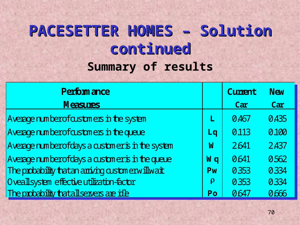
Average number of customers in the system L 0.467 0.435Average number of customers in the queue Lq 0.113 0.100Average number of days a customer is in the system W 2.641 2.437Average number of days a customer is in the queue Wq 0.641 0.562The probability that an arriving customer will wait Pw 0.353 0.334Oveall system effective utilization-factor 0.353 0.334The probability that all servers are idle Po 0.647 0.666
Performance Current New
Measures Car Car
Average number of customers in the system L 0.467 0.435Average number of customers in the queue Lq 0.113 0.100Average number of days a customer is in the system W 2.641 2.437Average number of days a customer is in the queue Wq 0.641 0.562The probability that an arriving customer will wait Pw 0.353 0.334Oveall system effective utilization-factor 0.353 0.334The probability that all servers are idle Po 0.647 0.666
Summary of results
PACESETTER HOMES – Solution PACESETTER HOMES – Solution continuedcontinued

71
PACESETTER HOMES – PACESETTER HOMES –
Spreadsheet SolutionSpreadsheet Solution
M/M/1//m Queuing Model
INPUTS Value0.05
Mu = 0.533334
Probabiility of n Customers OUTPUTS in the System where n =# Servers L Lq W Wq Pw Rho 0 1 2 3 4
1 0.43451 0.10025 2.43734 0.56233 0.33427 0.33427 0.66573 0.24965 0.07021 0.01317 0.00123
Lambda =
m =
72
9.9 Economic Analysis of 9.9 Economic Analysis of Queuing SystemsQueuing Systems
• The performance measures previously developed are used next to determine a minimal cost queuing system.
• The procedure requires estimated costs such as: – Hourly cost per server .– Customer goodwill cost while waiting in line. – Customer goodwill cost while being served.
73
WILSON FOODS WILSON FOODS TALKING TURKEY HOT LINETALKING TURKEY HOT LINE
• Wilson Foods has an 800 number to answer customers’ questions.
• If all the customer representatives are busy when a new customer calls, he/she is asked to stay on the line.
• A customer stays on the line if the waiting time is not longer than 3 minutes.
74
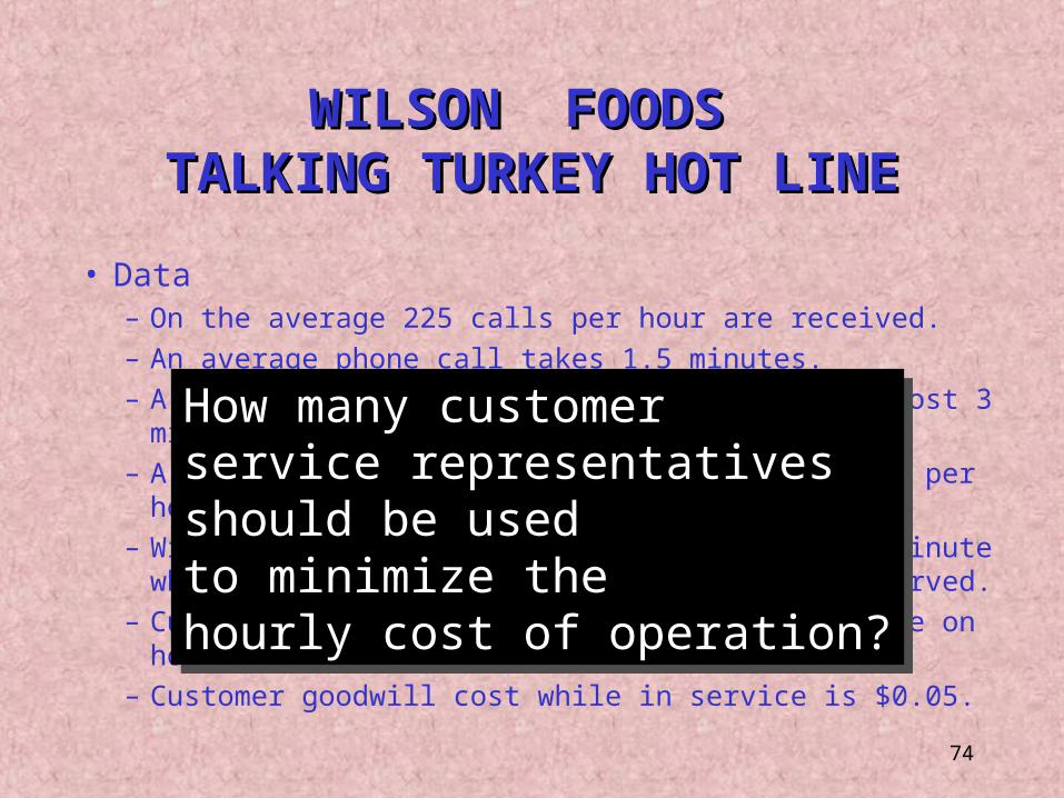
• Data– On the average 225 calls per hour are received.– An average phone call takes 1.5 minutes.– A customer will stay on the line waiting at most 3 minutes.– A customer service representative is paid $16 per hour.– Wilson pays the telephone company $0.18 per minute when the
customer is on hold or when being served.– Customer goodwill cost is $20 per minute while on hold.– Customer goodwill cost while in service is $0.05.
How many customer service representatives should be usedto minimize the hourly cost of operation?
How many customer service representatives should be usedto minimize the hourly cost of operation?
WILSON FOODS WILSON FOODS TALKING TURKEY HOT LINETALKING TURKEY HOT LINE
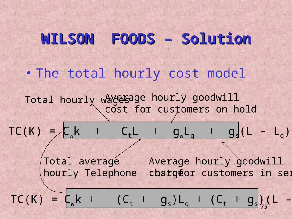
75TC(K) = Cwk + (Ct + gs)Lq + (Ct + gs)(L – Lq)
WILSON FOODS – SolutionWILSON FOODS – Solution
• The total hourly cost model
TC(K) = Cwk + CtL + gwLq + gs(L - Lq)
Total hourly wages
Total average hourly Telephone charge
Average hourly goodwill cost for customers on hold
Average hourly goodwillcost for customers in service
76
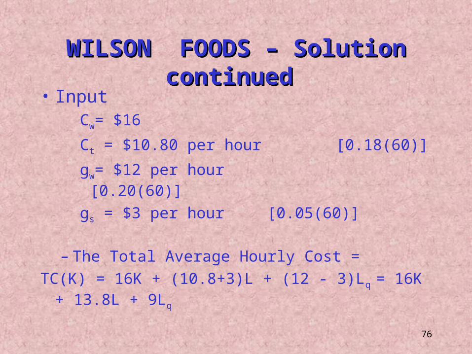
• InputCw= $16
Ct = $10.80 per hour [0.18(60)]
gw= $12 per hour [0.20(60)]
gs = $3 per hour [0.05(60)]
– The Total Average Hourly Cost =TC(K) = 16K + (10.8+3)L + (12 - 3)Lq = 16K + 13.8L + 9Lq
WILSON FOODS – Solution continued WILSON FOODS – Solution continued
77
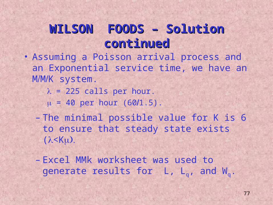
• Assuming a Poisson arrival process and an Exponential service time, we have an MMK system.
= 225 calls per hour. = 40 per hour (601.5).
– The minimal possible value for K is 6 to ensure that steady state exists (<K
– Excel MMk worksheet was used to generate results for L, Lq, and Wq.
WILSON FOODS – Solution continuedWILSON FOODS – Solution continued
78
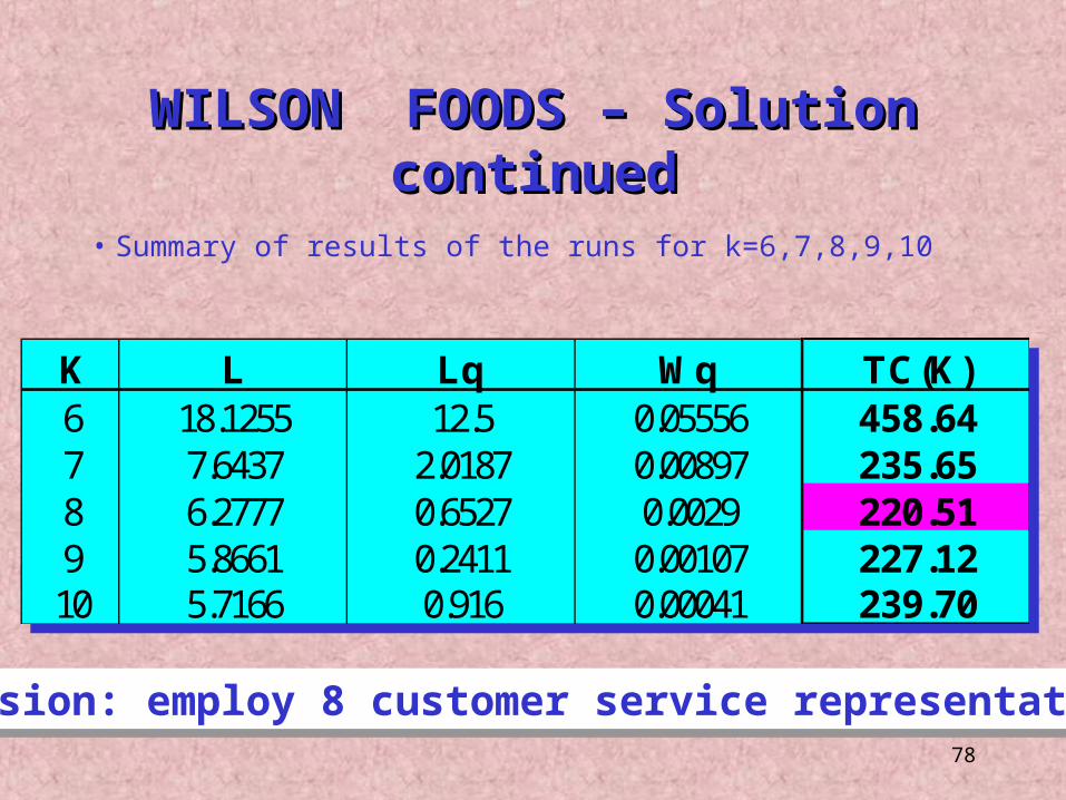
• Summary of results of the runs for k=6,7,8,9,10
K L Lq Wq TC(K)6 18.1255 12.5 0.05556 458.647 7.6437 2.0187 0.00897 235.658 6.2777 0.6527 0.0029 220.519 5.8661 0.2411 0.00107 227.1210 5.7166 0.916 0.00041 239.70
K L Lq Wq TC(K)6 18.1255 12.5 0.05556 458.647 7.6437 2.0187 0.00897 235.658 6.2777 0.6527 0.0029 220.519 5.8661 0.2411 0.00107 227.1210 5.7166 0.916 0.00041 239.70
Conclusion: employ 8 customer service representatives.Conclusion: employ 8 customer service representatives.
WILSON FOODS – Solution continuedWILSON FOODS – Solution continued
79
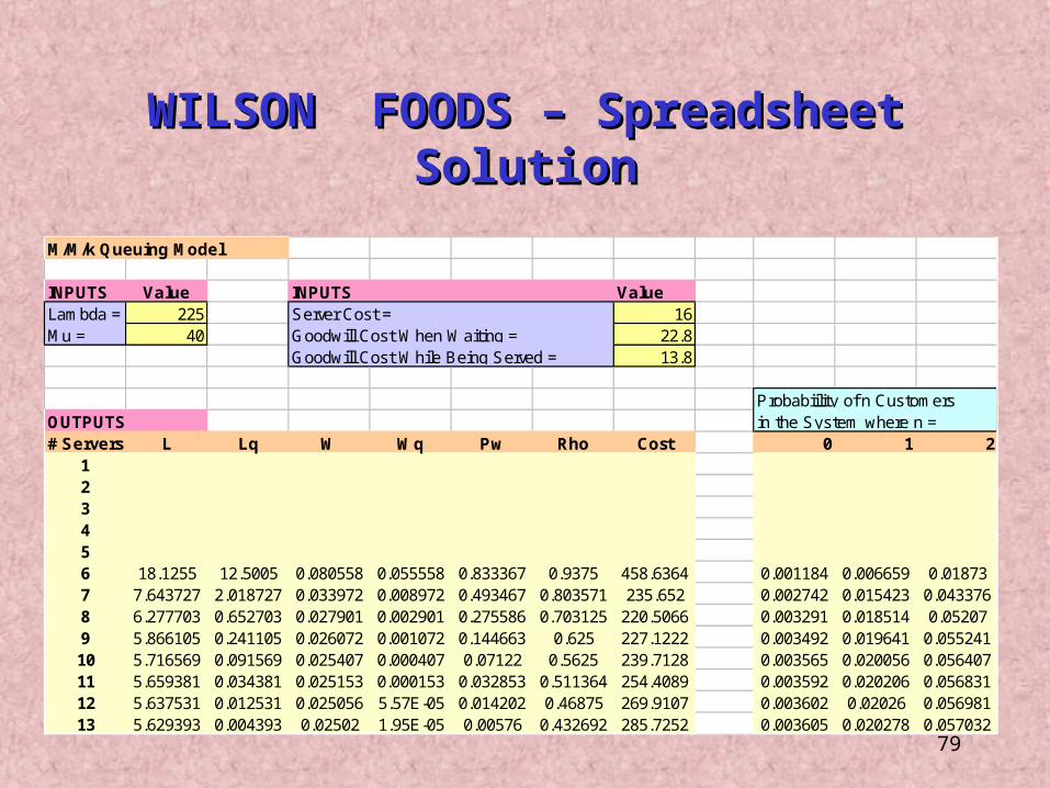
WILSON FOODS – Spreadsheet SolutionWILSON FOODS – Spreadsheet Solution
M/M/k Queuing Model
INPUTS Value INPUTS ValueLambda = 225 16Mu = 40 22.8
13.8
OUTPUTS# Servers L Lq W Wq Pw Rho Cost 0 1 2
123456 18.1255 12.5005 0.080558 0.055558 0.833367 0.9375 458.6364 0.001184 0.006659 0.018737 7.643727 2.018727 0.033972 0.008972 0.493467 0.803571 235.652 0.002742 0.015423 0.0433768 6.277703 0.652703 0.027901 0.002901 0.275586 0.703125 220.5066 0.003291 0.018514 0.052079 5.866105 0.241105 0.026072 0.001072 0.144663 0.625 227.1222 0.003492 0.019641 0.05524110 5.716569 0.091569 0.025407 0.000407 0.07122 0.5625 239.7128 0.003565 0.020056 0.05640711 5.659381 0.034381 0.025153 0.000153 0.032853 0.511364 254.4089 0.003592 0.020206 0.05683112 5.637531 0.012531 0.025056 5.57E-05 0.014202 0.46875 269.9107 0.003602 0.02026 0.05698113 5.629393 0.004393 0.02502 1.95E-05 0.00576 0.432692 285.7252 0.003605 0.020278 0.057032
in the System where n =Probabiility of n Customers
Server Cost =Goodwill Cost When Waiting =Goodwill Cost While Being Served =
80
HARGROVE HOSPITAL MATERNITY HARGROVE HOSPITAL MATERNITY WARDWARD
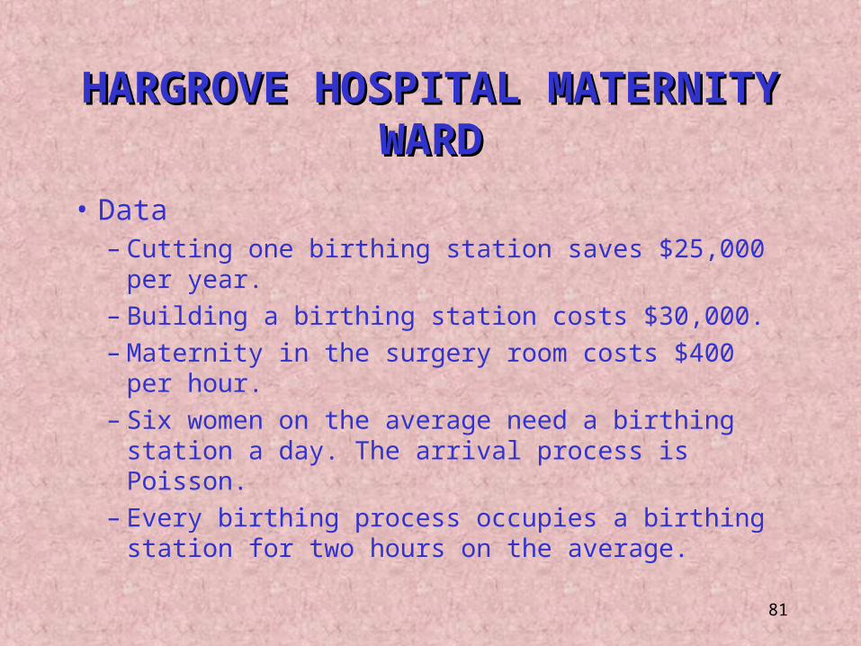
• Hargrove Hospital is experiencing cutbacks, and is trying to reorganize operations to reduce operating costs.
• There is a trade off between – the costs of operating more birthing stations and – the costs of rescheduling surgeries in the surgery room when
women give birth there, if all the birthing stations are occupied.
• The hospital wants to determine the optimal number of birthing stations that will minimize operating costs.
81
HARGROVE HOSPITAL MATERNITY HARGROVE HOSPITAL MATERNITY WARDWARD
• Data– Cutting one birthing station saves $25,000 per year.– Building a birthing station costs $30,000.– Maternity in the surgery room costs $400 per hour.– Six women on the average need a birthing station a
day. The arrival process is Poisson.– Every birthing process occupies a birthing station for
two hours on the average.
82
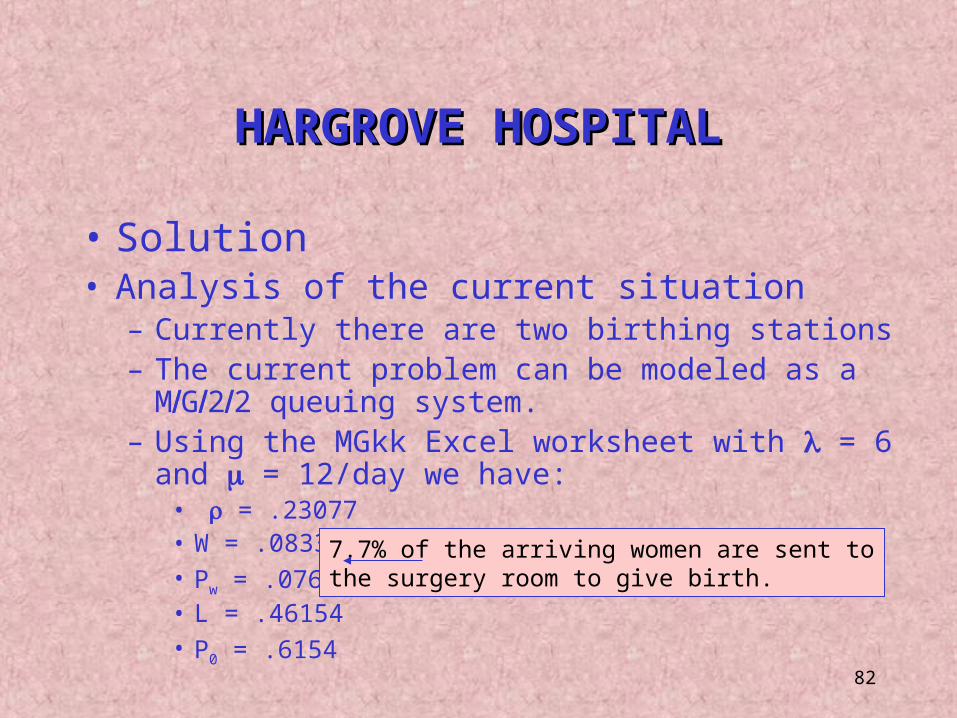
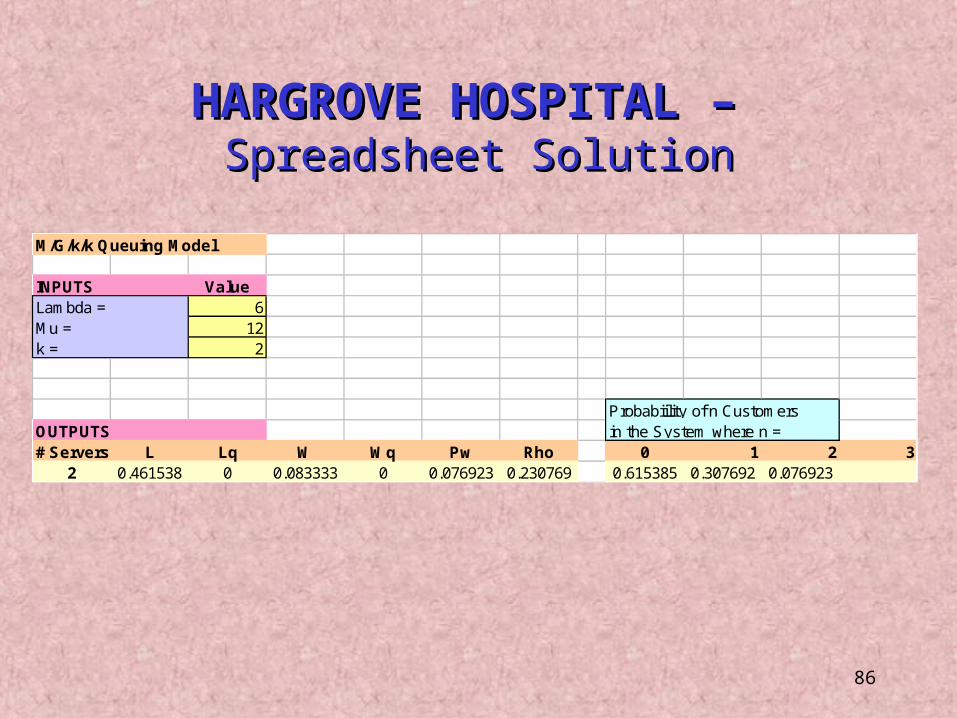
• Solution• Analysis of the current situation
– Currently there are two birthing stations– The current problem can be modeled as a MG22 queuing
system.– Using the MGkk Excel worksheet with = 6 and = 12/day we
have:• = .23077• W = .0833 days• Pw = .076923• L = .46154• P0 = .6154
HARGROVE HOSPITALHARGROVE HOSPITAL
7.7% of the arriving women are sent tothe surgery room to give birth.
83
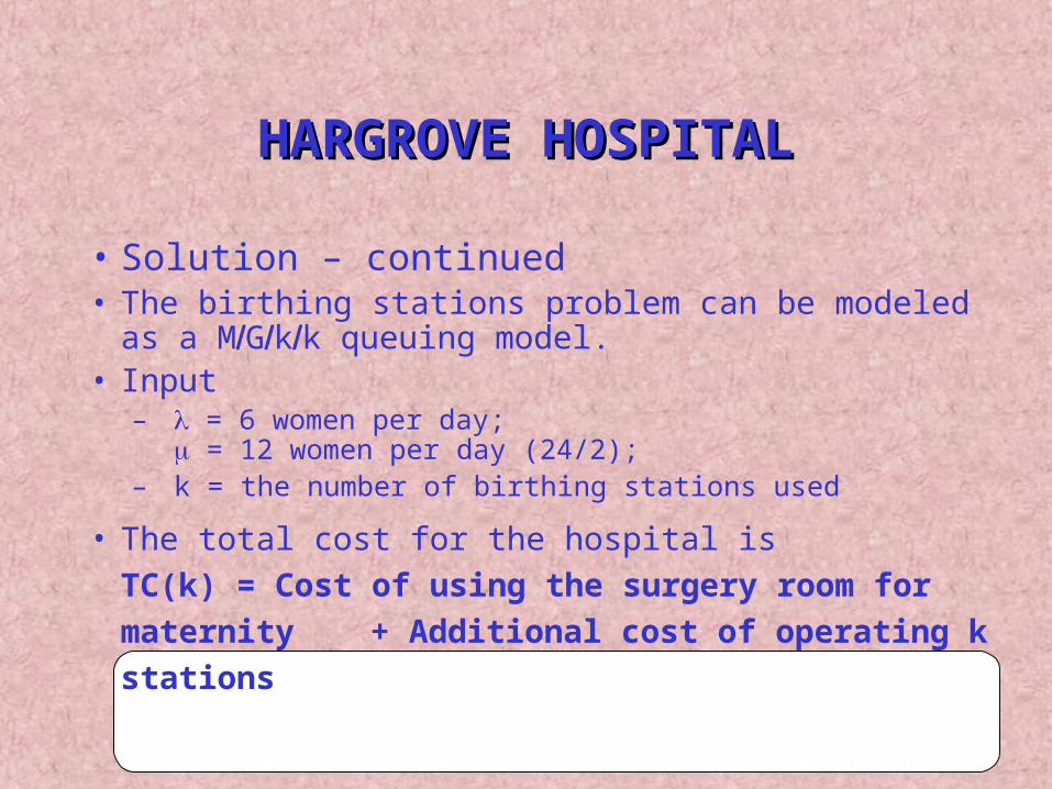
• Solution – continued • The birthing stations problem can be modeled as a MGkk
queuing model.• Input
– = 6 women per day; = 12 women per day (24/2);
– k = the number of birthing stations used
• The total cost for the hospital isTC(k) = Cost of using the surgery room for maternity
+ Additional cost of operating k stations
HARGROVE HOSPITALHARGROVE HOSPITAL
84
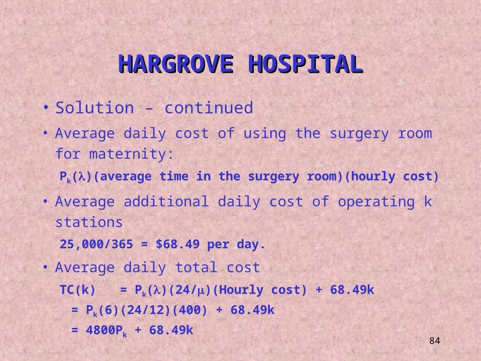
• Solution – continued • Average daily cost of using the surgery room for maternity:
Pk()(average time in the surgery room)(hourly cost)
• Average additional daily cost of operating k stations25,000/365 = $68.49 per day.
• Average daily total costTC(k) = Pk()(24/)(Hourly cost) + 68.49k
= Pk(6)(24/12)(400) + 68.49k
= 4800Pk + 68.49k
HARGROVE HOSPITALHARGROVE HOSPITAL
85
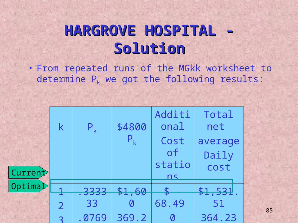
k Pk $4800Pk
AdditionalCost of stations
Total net average Daily cost
1234
.333333
.076923
.012658
.001580
$1,600369.2360.767.58
$ – 68.49 0
82.19163.38
$1,531.51364.23142.95171.96
Optimal
• From repeated runs of the MGkk worksheet to determine Pk we got the following results:
HARGROVE HOSPITAL - SolutionHARGROVE HOSPITAL - Solution
Current
86
HARGROVE HOSPITAL – HARGROVE HOSPITAL – Spreadsheet SolutionSpreadsheet Solution
M/G/k/k Queuing Model
INPUTS Value6
122
OUTPUTS# Servers L Lq W Wq Pw Rho 0 1 2 3
2 0.461538 0 0.083333 0 0.076923 0.230769 0.615385 0.307692 0.076923
in the System where n =Probabiility of n Customers
Lambda =Mu =k =
87
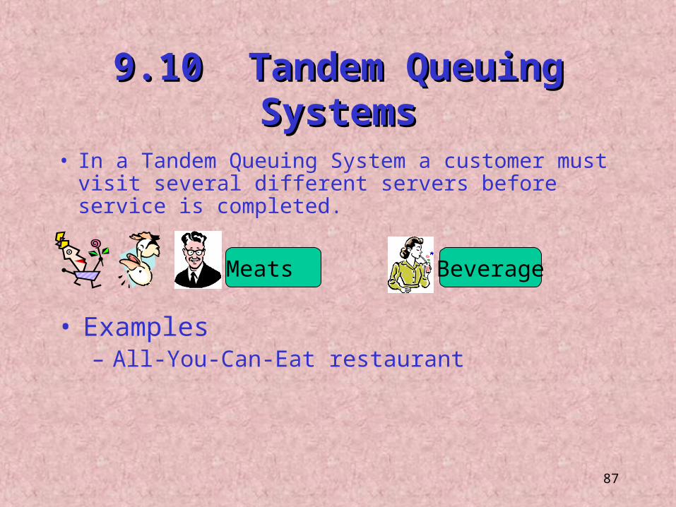
9.10 Tandem Queuing Systems9.10 Tandem Queuing Systems
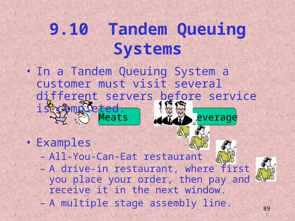
• In a Tandem Queuing System a customer must visit several different servers before service is completed.
Beverage Meats
• Examples– All-You-Can-Eat restaurant
88
Beverage Meats
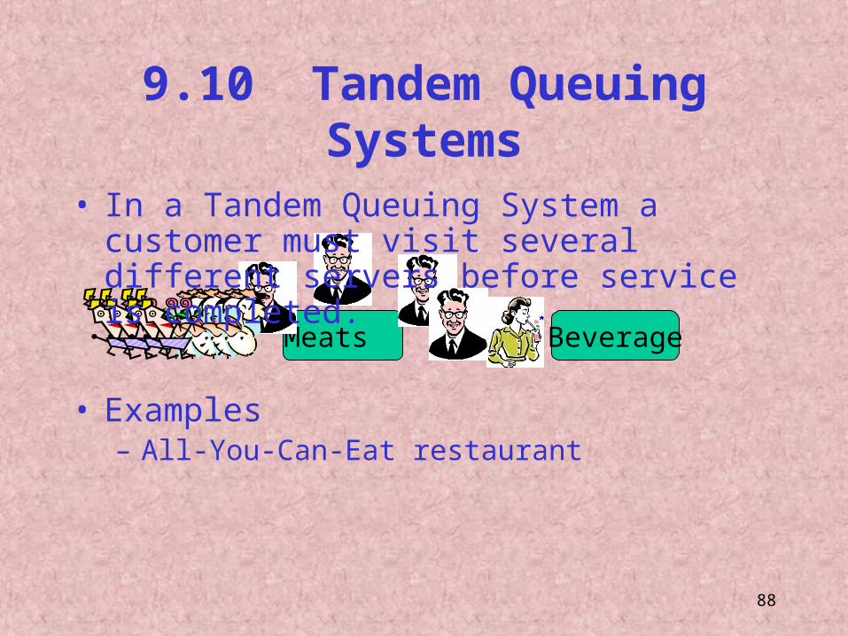
• In a Tandem Queuing System a customer must visit several different servers before service is completed.
9.10 Tandem Queuing Systems
• Examples– All-You-Can-Eat restaurant
89
Beverage Meats
9.10 Tandem Queuing Systems
– A drive-in restaurant, where first you place your order, then pay and receive it in the next window.
– A multiple stage assembly line.
• Examples– All-You-Can-Eat restaurant
• In a Tandem Queuing System a customer must visit several different servers before service is completed.
90
9.10 Tandem Queuing Systems9.10 Tandem Queuing Systems
• For cases in which customers arrive according to a Poisson process and service time in each station is exponential, ….
Total Average Time in the System = Sum of all average times at the individual stations
Total Average Time in the System = Sum of all average times at the individual stations
91
BIG BOYS SOUND, INC.BIG BOYS SOUND, INC.
• Big Boys sells audio merchandise.• The sale process is as follows:
– A customer places an order with a sales person.
– The customer goes to the cashier station to pay for the order.
– After paying, the customer is sent to the pickup desk to obtain the good.
92
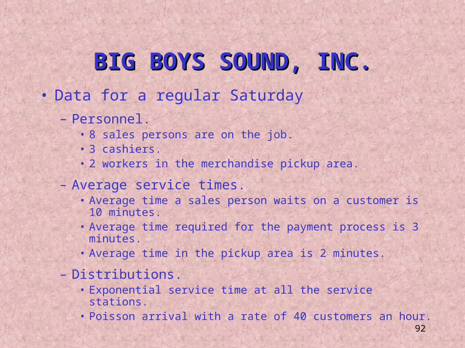
• Data for a regular Saturday– Personnel.
• 8 sales persons are on the job.• 3 cashiers.• 2 workers in the merchandise pickup area.
– Average service times.• Average time a sales person waits on a customer is 10 minutes.• Average time required for the payment process is 3 minutes.• Average time in the pickup area is 2 minutes.
– Distributions.• Exponential service time at all the service stations.• Poisson arrival with a rate of 40 customers an hour.
BIG BOYS SOUND, INC.BIG BOYS SOUND, INC.
93
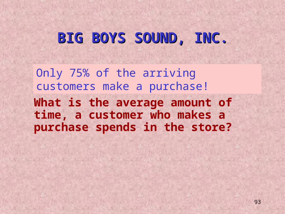
What is the average amount of time, a customer who makes a purchase spends in the store?
Only 75% of the arriving customers make a purchase!
BIG BOYS SOUND, INC.BIG BOYS SOUND, INC.
94
BIG BOYS SOUND, INC. – SolutionBIG BOYS SOUND, INC. – Solution
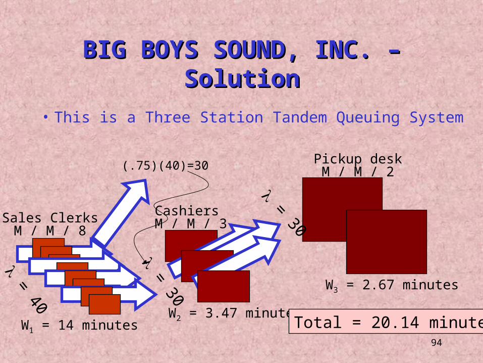
• This is a Three Station Tandem Queuing System
Sales ClerksM / M / 8
CashiersM / M / 3
Pickup deskM / M / 2
= 40
= 30
= 30
W1 = 14 minutesW2 = 3.47 minutes
W3 = 2.67 minutes
Total = 20.14 minutes.
(.75)(40)=30
95
Appendix : Assembly Line BalancingAppendix : Assembly Line Balancing
• An Assembly Line can be thought of as a tandem queue, because a product visits several workstations in a given sequence.
• In a balanced assembly line the time spent in each of the different workstations is about the same.
• The objective is to maximize production throughput by allocating tasks to workstations
96
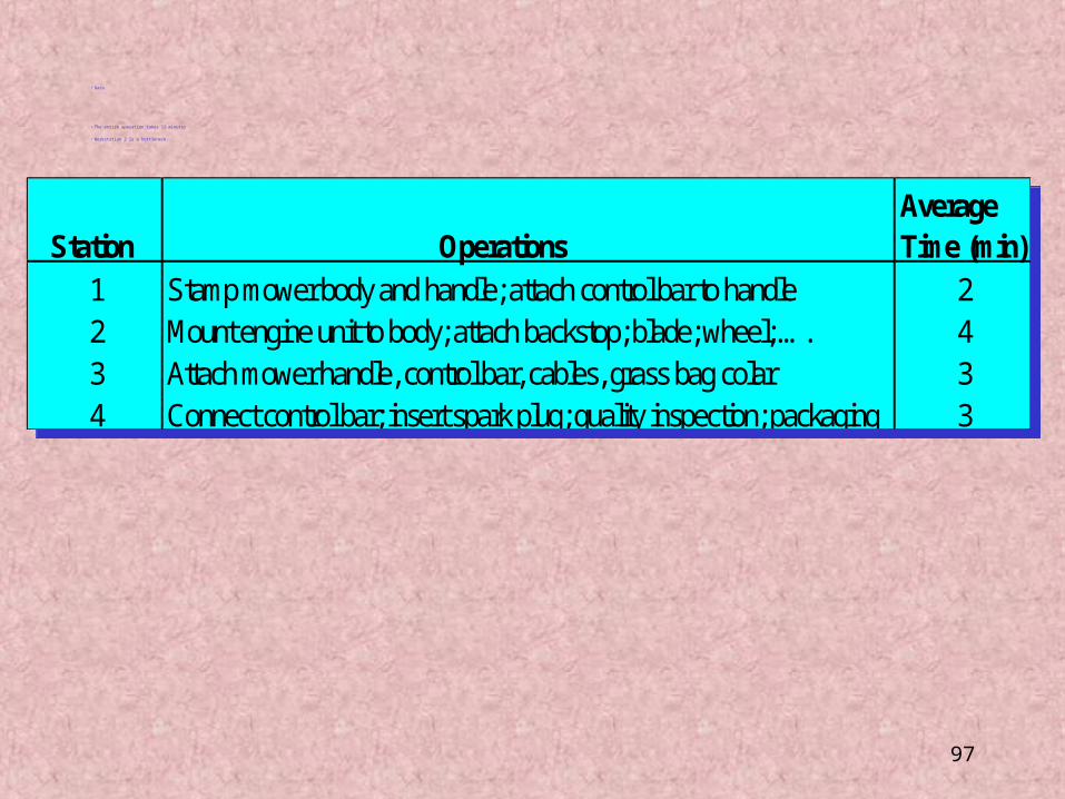
McMURRAY MACHINE COMPANYMcMURRAY MACHINE COMPANY
• McMurray manufactures lawn mowers and snow blowers.• The assembly operation of a certain mower consists of four
workstations.• The longest time spent at a workstation is 4 minutes. Thus,
the maximum number of mowers that can be produced is 15 per hour.
• Management would like to increase productivity by better balancing the assembly line.
97
• Data
• The entire operation takes 12 minutes
• Workstation 2 is a bottleneck.
Average Station Operations Time (min)
1 Stamp mower body and handle; attach control bar to handle 22 Mount engine unit to body; attach backstop; blade; wheel; …. 43 Attach mower handle, control bar, cables, grass bag colar 34 Connect control bar; insert spark plug; quality inspection; packaging 3
Average Station Operations Time (min)
1 Stamp mower body and handle; attach control bar to handle 22 Mount engine unit to body; attach backstop; blade; wheel; …. 43 Attach mower handle, control bar, cables, grass bag colar 34 Connect control bar; insert spark plug; quality inspection; packaging 3
98
SOLUTIONSOLUTION
• Various options to balance the assembly line– Try to schedule operations to take a total of three
minutes in each station .
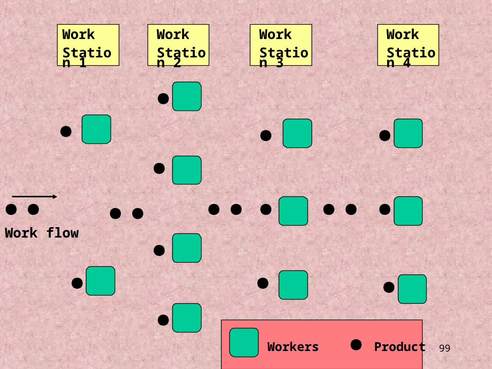
– Assign workers to workstations as needed to balance the station outputs.
– Assign multiple workstations to perform the operations.
99
WorkStation 4
WorkStation 1
WorkStation 2
WorkStation 3
Work flow
Workers Product
100
– Use Integer and Dynamic Programming optimization techniques, to minimize the total amount of idle time at all workstations.
– Use an heuristic techniques such as “The Ranked Position Weight Technique,” to find the smallest number of workstations needed to meet a prespecified cycle time.
• (Although a heuristic solution does not guarantee optimality, this heuristic was found optimal in large number of applications.)
101
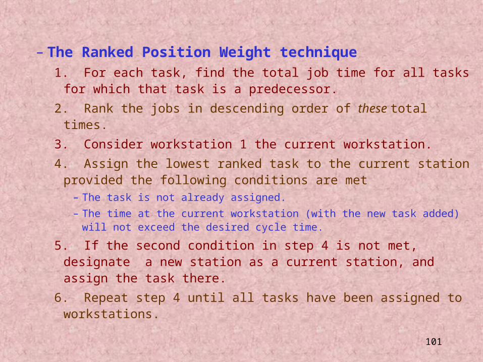
– The Ranked Position Weight technique1. For each task, find the total job time for all tasks for which that task is
a predecessor.
2. Rank the jobs in descending order of these total times.
3. Consider workstation 1 the current workstation.
4. Assign the lowest ranked task to the current station provided the following conditions are met
– The task is not already assigned.– The time at the current workstation (with the new task added) will not exceed
the desired cycle time.
5. If the second condition in step 4 is not met, designate a new station as a current station, and assign the task there.
6. Repeat step 4 until all tasks have been assigned to workstations.
102
McMURRAY - continuedMcMURRAY - continued
• Demand for the mower increased, and as a result the needed cycle time drops to 3 minutes in the assembly line.
• McMurray would like to balance the line using the smallest number of workstations.
103
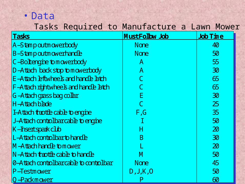
• Data
Tasks Must Follow Job Job TimeA--Stamp out mower body None 40B--Stamp out mower handle None 50C--Bolt engine to mower body A 55D--Attach back stop to mower body A 30E--Attach left wheels and handle latch C 65F--Attach right wheels and handle latch C 65G--Attach grass bag collar E 30H--Attach blade C 25I--Attach throttle cable to engine F, G 35J--Attach control bar cable to engine I 50K--Insert spark club H 20L--Attach control bar to handle B 30M--Attach handle to mower L 20N--Attach throttle cable to handle M 500--Attach control bar cable to control bar None 45P--Test mower D, J, K, O 50Q--Pack mower P 60
Tasks Must Follow Job Job TimeA--Stamp out mower body None 40B--Stamp out mower handle None 50C--Bolt engine to mower body A 55D--Attach back stop to mower body A 30E--Attach left wheels and handle latch C 65F--Attach right wheels and handle latch C 65G--Attach grass bag collar E 30H--Attach blade C 25I--Attach throttle cable to engine F, G 35J--Attach control bar cable to engine I 50K--Insert spark club H 20L--Attach control bar to handle B 30M--Attach handle to mower L 20N--Attach throttle cable to handle M 500--Attach control bar cable to control bar None 45P--Test mower D, J, K, O 50Q--Pack mower P 60
Tasks Required to Manufacture a Lawn Mower
104
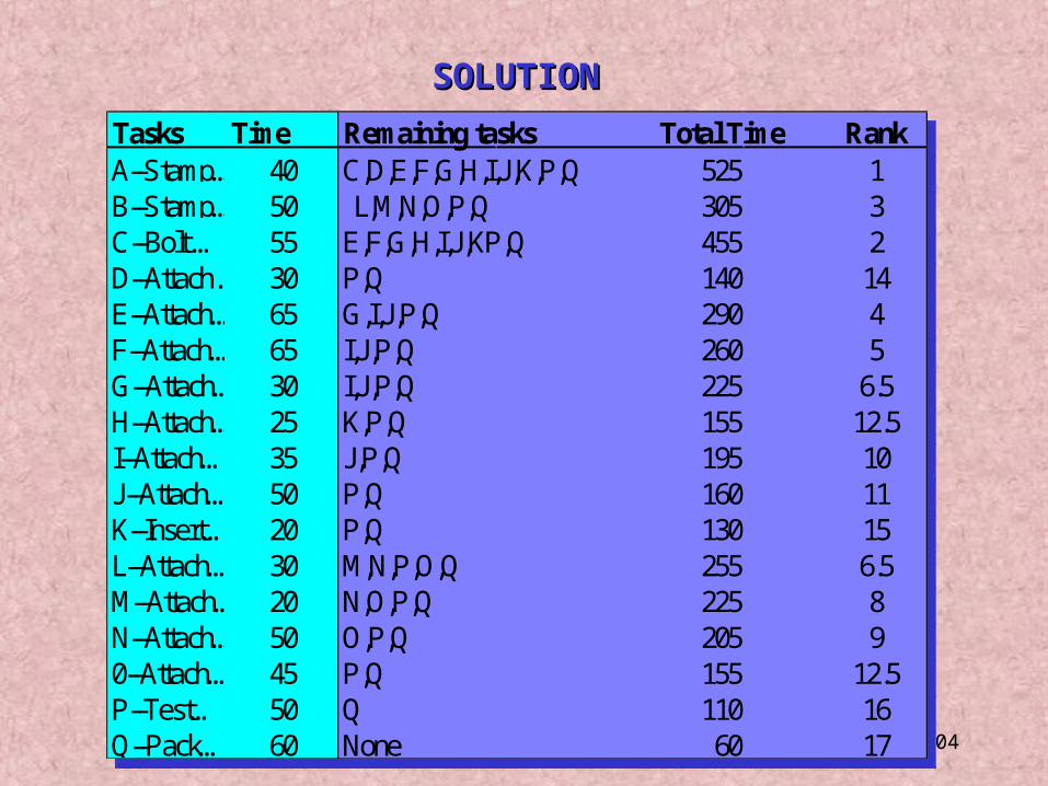
SOLUTIONSOLUTION
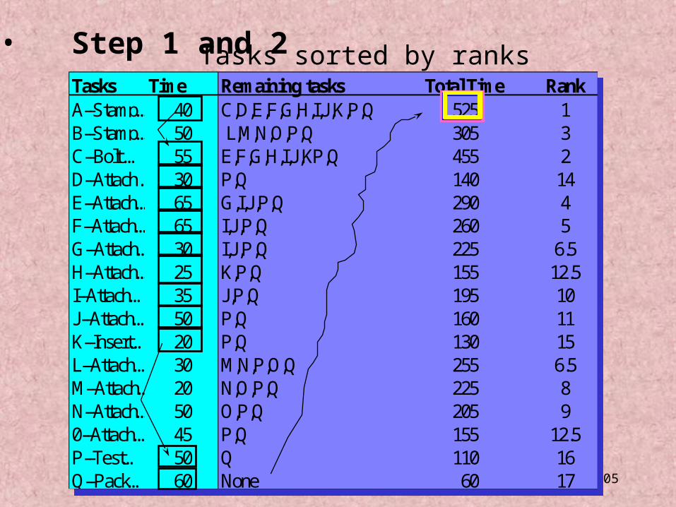
Tasks Time Remaining tasks Total Time RankA--Stamp… 40 C,D,E,F,G,H,I,J,K,P,Q 525 1B--Stamp… 50 L,M,N,O,P,Q 305 3C--Bolt … 55 E,F,G,H,I,J,KP,Q 455 2D--Attach … 30 P,Q 140 14E--Attach… 65 G,I,J,P,Q 290 4F--Attach… 65 I,J,P,Q 260 5G--Attach… 30 I,J,P,Q 225 6.5H--Attach… 25 K,P,Q 155 12.5I--Attach… 35 J,P,Q 195 10J--Attach… 50 P,Q 160 11K--Insert… 20 P,Q 130 15L--Attach… 30 M,N,P,O,Q 255 6.5M--Attach… 20 N,O,P,Q 225 8N--Attach… 50 O,P,Q 205 90--Attach… 45 P,Q 155 12.5P--Test… 50 Q 110 16Q--Pack… 60 None 60 17
Tasks Time Remaining tasks Total Time RankA--Stamp… 40 C,D,E,F,G,H,I,J,K,P,Q 525 1B--Stamp… 50 L,M,N,O,P,Q 305 3C--Bolt … 55 E,F,G,H,I,J,KP,Q 455 2D--Attach … 30 P,Q 140 14E--Attach… 65 G,I,J,P,Q 290 4F--Attach… 65 I,J,P,Q 260 5G--Attach… 30 I,J,P,Q 225 6.5H--Attach… 25 K,P,Q 155 12.5I--Attach… 35 J,P,Q 195 10J--Attach… 50 P,Q 160 11K--Insert… 20 P,Q 130 15L--Attach… 30 M,N,P,O,Q 255 6.5M--Attach… 20 N,O,P,Q 225 8N--Attach… 50 O,P,Q 205 90--Attach… 45 P,Q 155 12.5P--Test… 50 Q 110 16Q--Pack… 60 None 60 17
105
Tasks Time Remaining tasks Total Time RankA--Stamp… 40 C,D,E,F,G,H,I,J,K,P,Q 525 1B--Stamp… 50 L,M,N,O,P,Q 305 3C--Bolt … 55 E,F,G,H,I,J,KP,Q 455 2D--Attach … 30 P,Q 140 14E--Attach… 65 G,I,J,P,Q 290 4F--Attach… 65 I,J,P,Q 260 5G--Attach… 30 I,J,P,Q 225 6.5H--Attach… 25 K,P,Q 155 12.5I--Attach… 35 J,P,Q 195 10J--Attach… 50 P,Q 160 11K--Insert… 20 P,Q 130 15L--Attach… 30 M,N,P,O,Q 255 6.5M--Attach… 20 N,O,P,Q 225 8N--Attach… 50 O,P,Q 205 90--Attach… 45 P,Q 155 12.5P--Test… 50 Q 110 16Q--Pack… 60 None 60 17
Tasks Time Remaining tasks Total Time RankA--Stamp… 40 C,D,E,F,G,H,I,J,K,P,Q 525 1B--Stamp… 50 L,M,N,O,P,Q 305 3C--Bolt … 55 E,F,G,H,I,J,KP,Q 455 2D--Attach … 30 P,Q 140 14E--Attach… 65 G,I,J,P,Q 290 4F--Attach… 65 I,J,P,Q 260 5G--Attach… 30 I,J,P,Q 225 6.5H--Attach… 25 K,P,Q 155 12.5I--Attach… 35 J,P,Q 195 10J--Attach… 50 P,Q 160 11K--Insert… 20 P,Q 130 15L--Attach… 30 M,N,P,O,Q 255 6.5M--Attach… 20 N,O,P,Q 225 8N--Attach… 50 O,P,Q 205 90--Attach… 45 P,Q 155 12.5P--Test… 50 Q 110 16Q--Pack… 60 None 60 17
Tasks sorted by ranks• Step 1 and 2
106
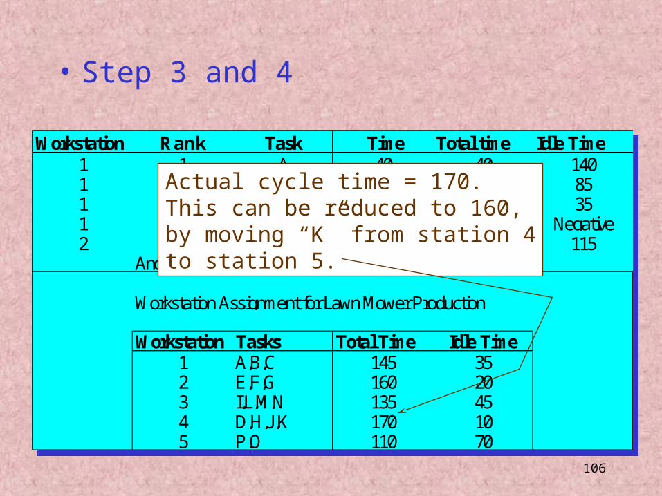
• Step 3 and 4
Workstation Rank Task Time Total time Idle Time1 1 A 40 40 1401 2 C 55 95 851 3 B 50 145 351 4 E 65 210 Negative2 4 E 65 65 115
And so on….
Workstation Assignment for Lawn Mower Production
Workstation Tasks Total Time Idle Time1 A,B,C 145 352 E,F,G 160 203 I,L,M,N 135 454 D,H,J,K 170 105 P,Q 110 70
Workstation Rank Task Time Total time Idle Time1 1 A 40 40 1401 2 C 55 95 851 3 B 50 145 351 4 E 65 210 Negative2 4 E 65 65 115
And so on….
Workstation Assignment for Lawn Mower Production
Workstation Tasks Total Time Idle Time1 A,B,C 145 352 E,F,G 160 203 I,L,M,N 135 454 D,H,J,K 170 105 P,Q 110 70
Actual cycle time = 170.This can be reduced to 160,by moving “K” from station 4to station 5.


