24
1
A New Heuristic for
Rectilinear Steiner Trees
Ion I. M�andoiu, Vijay V. Vazirani, and Joseph L. Ganley
Abstract
The minimum rectilinear Steiner tree (RST) problem is one of the fundamental problems in the
�eld of electronic design automation. The problem is NP-hard, and much work has been devoted to
designing good heuristics and approximation algorithms; to date, the champion in solution quality
among RST heuristics is the Batched Iterated 1-Steiner (BI1S) heuristic of Kahng and Robins. In
a recent development, exact RST algorithms have witnessed spectacular progress: The new release
of the GeoSteiner code of Warme, Winter, and Zachariasen has average running time comparable
to that of the fastest available BI1S implementation, due to Robins. We are thus faced with the
paradoxical situation that an exact algorithm for an NP-hard problem is competitive in speed with
a state-of-the-art heuristic for the problem.
The main contribution of this paper is a new RST heuristic, which has at its core a recent 3/2
approximation algorithm of Rajagopalan and Vazirani for the metric Steiner tree problem on quasi-
bipartite graphs|these are graphs that do not contain edges connecting pairs of Steiner vertices.
The RV algorithm is built around the linear programming relaxation of a sophisticated integer
program formulation, called the bidirected cut relaxation. Our heuristic achieves a good running
time by combining an e�cient implementation of the RV algorithm with simple, but powerful
geometric reductions.
Experiments conducted on both random and real VLSI instances show that the new RST
heuristic runs signi�cantly faster than Robins' implementation of BI1S and than the GeoSteiner
code. Moreover, the new heuristic typically gives higher-quality solutions than BI1S.
Keywords
Routing, interconnect synthesis, Steiner tree, optimization.
The work of the �rst two authors was supported by NSF Grant CCR 9627308.
I. I. M�andoiu and V. V. Vazirani are with College of Computing, Georgia Institute of Technology, Atlanta, GA
30332, USA. E-mail: fmandoiu,[email protected].
J. L. Ganley is with Simplex Solutions, Inc., 521 Almanor Avenue, Sunnyvale, CA 94086, USA. E-mail:
2I. Introduction
The Steiner tree problem is that of �nding a minimum-length interconnection of a set of
terminals, and has long been one of the fundamental problems in the �eld of electronic
design automation. Although recent advances of integrated circuit technology into the
deep-submicron realm have introduced additional routing objective functions, the Steiner
tree problem retains its importance: For non-critical nets, or in physically small instances,
minimum length is still frequently a good objective function, since a minimum-length in-
terconnection has minimum overall capacitance and occupies a minimum amount of area.
Furthermore, the development of good algorithms for the Steiner tree problem often lays a
foundation for expanding these algorithms to accommodate objective functions other than
purely minimizing length.
The rectilinear Steiner tree (RST) problem|in which the terminals are points in the plane
and distances between them are measured in the L1 metric|has been the most-examined
variant in electronic design automation, since IC fabrication technology typically mandates
the use of only horizontal and vertical interconnect. The RST problem is NP-hard [10], and
much e�ort has been devoted to designing heuristic and approximation algorithms [1], [2],
[3], [6], [11], [14], [16], [18], [19], [20], [30], [31], [32]. In an extensive survey of RST heuristics
up to 1992 [17], the Batched Iterated 1-Steiner (BI1S) heuristic of Kahng and Robins [18]
emerged as the clear winner with an average improvement over the MST on terminals of
almost 11%. Subsequently, two other heuristics [3], [19] have been reported to match the
same performance.
After a steady, but relatively slow progress [5], [8], [25], exact RST algorithms have recently
witnessed spectacular progress [28] (see also [7]). The new release [29] of the GeoSteiner code
by Warme, Winter, and Zachariasen has average running time comparable to the fast BI1S
implementation of Robins [22] on random instances. We are thus faced with the paradoxical
situation that an exact algorithm for an NP-hard problem has the same average running
time as a state-of-the-art heuristic for the problem. It appears that, for the RST problem,
progress on heuristics has lagged behind that on exact algorithms.
We try to remedy this situation by proposing a new RST heuristic. Our experiments show
that the new heuristic has better average running time than both Robins' implementation
of BI1S and the GeoSteiner code. Moreover, the new heuristic gives higher-quality solutions
3than BI1S on the average; of course, it cannot beat GeoSteiner in solution quality.
Our results are obtained by exploiting a number of recent algorithmic and implementation
ideas. On the algorithmic side, we build on the recent 3=2 approximation algorithm of Ra-
jagopalan and Vazirani [21] for the metric Steiner tree problem on quasi-bipartite graphs;
these are graphs that do not contain edges connecting pairs of Steiner vertices. This algo-
rithm is based on the linear programming relaxation of a sophisticated integer formulation of
the metric Steiner tree problem, called the bidirected cut formulation. It is well known that
the RST problem can be reduced to the metric Steiner tree problem on graphs [13], however,
the graphs obtained from the reduction are not quasi-bipartite. We give an RV-based heuris-
tic for �nding Steiner trees in arbitrary (non quasi-bipartite) metric graphs. The heuristic,
called Iterated RV (IRV), computes a Steiner tree of a quasi-bipartite subgraph of the original
graph using the RV algorithm, in order to select a set of candidate Steiner vertices. The
process is repeated with the selected Steiner vertices treated as terminals|thereby allowing
the algorithm to pick larger quasi-bipartite subgraphs, and seek additional Steiner vertices
for inclusion in the tree|until no further improvement is possible.
The e�cient implementation of the IRV heuristic depends critically on the size of the
quasi-bipartite subgraphs considered in each iteration. We decrease the size of the graphs
that correspond to RST instances by applying reductions, which are deletions of edges and
vertices that do not a�ect the quality of the result. Our key edge reduction is based on
Robins and Salowe's result that bounds the maximum degree of a rectilinear MST [23],
and allows us to retain in the graph at most 4 edges incident to each vertex. Notably, the
same reduction is the basis of a signi�cant speed-up in the running time of BI1S [12], and is
currently incorporated in Robins' implementation [22]. Our vertex reduction is based on a
simple empty rectangle test that has its roots in the work of Berman and Ramaiyer [2] (see
also [6], [31]).
We ran experiments to compare our implementation of IRV against Robins' implementa-
tion of BI1S [22] and against the GeoSteiner code of Warme, Winter, and Zachariasen [29].
The results reported in Section IV show that, on both random and real VLSI instances,
our new heuristic produces on the average higher-quality solutions than BI1S. The quality
improvement is not spectacular, around 0.03% from the cost of the MST, but we should
note that solutions produced by BI1S are already less than 0.5% away from optimum on the
4average.
More importantly, IRV's improvement in solution quality is achieved with an excellent
running time. On random instances with up to 250 terminals, our IRV code runs 4{10
times faster than the lp solve based version of GeoSteiner used in our experiments, and
2{10 times faster than Robins' implementation of BI1S|the speed-up increases with the
number of terminals. After noticing that BI1S can also bene�t from vertex reductions, we
incorporated the empty rectangle test into Robins' BI1S code. The enhanced BI1S code
becomes about 30% faster than our IRV code on large random instances. However, this
does not necessarily mean that BI1S is the best heuristic in practice. Results on real VLSI
instances indicate a di�erent hierarchy: On these instances both IRV and GeoSteiner are
faster than the enhanced BI1S.
It is interesting to note that, due to poor performance and prohibitive running times, none
of the previous algorithms with proven guarantees for the Steiner tree problem in graphs [1],
[2], [11], [20], [32] was found suitable as the core algorithmic idea around which heuristics can
be built for use in the industry. Our adaptation of the RV algorithm �lls this void for the �rst
time, and points to the importance of drawing on the powerful new ideas developed recently
in the emerging area of approximation algorithms for NP-hard optimization problems [26].
The remainder of this paper is structured as follows. Section II describes the RV algorithm
and its extension to non quasi-bipartite graphs. Section III describes how this extension,
IRV, is used to solve RST instances, and Section IV presents experimental results comparing
IRV with BI1S and GeoSteiner on test cases both randomly generated and extracted from
real circuit designs.
II. Steiner trees in graphs
The metric Steiner tree in graphs (GST) problem is: Given a connected graph G = (V;E)
whose vertices are partitioned in two sets, T and S, the terminal and Steiner vertices respec-
tively, and non-negative edge costs satisfying the triangle inequality, �nd a minimum cost
tree spanning all terminals and any subset of the Steiner vertices. Recently, Rajagopalan and
Vazirani [21] presented a 3/2 approximation algorithm (henceforth called the RV algorithm)
for the GST problem when restricted to quasi-bipartite graphs, i.e., graphs that have no edge
connecting a pair of Steiner vertices. In this section we review the RV algorithm, discuss
5its implementation, and present an RV-based heuristic for the GST problem on arbitrary
graphs.
A. The bidirected cut relaxation
The RV algorithm is based on a sophisticated integer programming (IP) formulation of
the GST problem. A related, but simpler formulation is given by the following observation:
A set of edges E0 � E connects terminals in T if and only if every cut of G separating two
terminals crosses at least one edge of E0. The IP formulation resulting from this observation
is called the undirected cut formulation. The IP formulation on which the RV algorithm is
based, called the bidirected cut formulation, is obtained by considering a directed version of
the above cut condition.
Let ~E be the set of arcs obtained by replacing each undirected edge (u; v) 2 E by two
directed arcs u ! v and v ! u. For a set C of vertices, let �(C) be the set of arcs u ! v
with u 2 C and v 2 V nC. Finally, if to is a �xed terminal, let C contain all sets C � V that
contain at least one terminal but do not contain to. The bidirected cut formulation attempts
to pick a minimum cost collection of arcs from ~E in such a way that each set in C has at
least one outgoing arc:
minimizeX
e2~E
cost(e)xe (1)
subject toX
e: e2�(C)
xe � 1; C 2 C
xe 2 f0; 1g; e 2 ~E
By allowing xe's to assume non-negative fractional values we obtain a linear program (LP)
called the bidirected cut relaxation of the GST problem:
minimizeX
e2~E
cost(e)xe (2)
subject toX
e: e2�(C)
xe � 1; C 2 C
xe � 0; e 2 ~E
The dual of the covering LP (2) is the packing LP:
6
maximizeX
C2C
yC (3)
subject toX
C: e2�(C)
yC � cost(e); e 2 ~E
yC � 0; C 2 C
From LP-duality theory, the cost of any feasible solution to (3) is less than or equal to the
cost of the optimum solution to (2), and hence, less than or equal to the cost of any feasible
solution to (1). The RV algorithm uses this observation to guarantee the quality of the
solution produced: The algorithm constructs feasible solutions to both IP (1) and LP (3),
in such a way that the costs of the two solutions di�er by at most a factor of 3/2.
B. The RV algorithm
The RV algorithm works on quasi-bipartite graphs G. At a coarse level, the RV algorithm
is similar to the Batched Iterated 1-Steiner algorithm of Kahng and Robins [18]: Both
algorithms work in phases, and in each phase some Steiner vertices are iteratively added to
the set of terminals. While BI1S adds Steiner vertices to T greedily|based on the decrease
in the cost of the MST|the RV algorithm uses the bidirected cut relaxation to guide the
addition.
In each phase, the RV algorithm constructs feasible solutions to both IP (1) and LP
(3). The bidirected cut formulation and its relaxation are inherently asymmetric, since
they require a terminal to to be singled out. However, the RV-Phase algorithm works in a
symmetric manner: The information it computes can be used to derive feasible solutions for
any choice of to.
A set C � V is called proper if both C and V n C contain terminals; with respect to
the original set of terminals only sets in C and their complements are proper. During its
execution, the RV-Phase algorithm tentatively converts some Steiner vertices into terminals;
note that the only proper sets created by these conversions are singleton sets containing
new terminals, and their complements. The algorithm maintains a variable yC , called dual ,
for every proper set, including the newly created ones. The amount of dual felt by arc e
isP
C : e2�(C) yC ; we say that e is tight whenP
C : e2�(C) yC = cost(e). A set C of vertices is
unsatis�ed if it is proper and �(C) does not contain any tight arc.
7
Input: Quasi-bipartite graph G and set T of terminals.
Output: Augmented set T .
1. ~L ;; For each proper set C, yC 0.
2. If all proper sets are satis�ed then return T and exit.
3. Uniformly rise the y values of minimally unsatis�ed sets until an arc u! v goes tight.
4. If u =2 T , then T T [ fug; repeat from Step 1.
5. Else, ~L ~L [ fu! vg; repeat from Step 2.
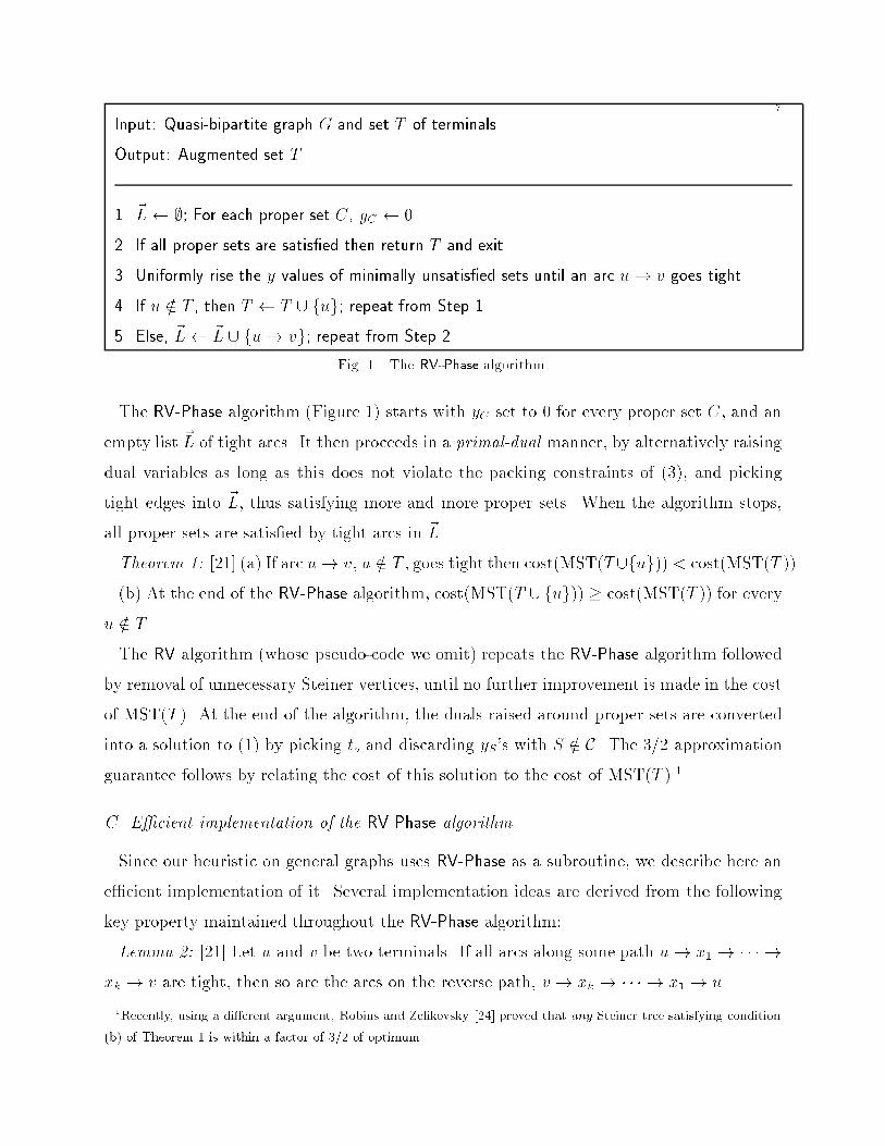
Fig. 1. The RV-Phase algorithm.
The RV-Phase algorithm (Figure 1) starts with yC set to 0 for every proper set C, and an
empty list ~L of tight arcs. It then proceeds in a primal-dual manner, by alternatively raising
dual variables as long as this does not violate the packing constraints of (3), and picking
tight edges into ~L, thus satisfying more and more proper sets. When the algorithm stops,
all proper sets are satis�ed by tight arcs in ~L.
Theorem 1: [21] (a) If arc u! v, u =2 T , goes tight then cost(MST(T[fug)) < cost(MST(T )).
(b) At the end of the RV-Phase algorithm, cost(MST(T [ fug)) � cost(MST(T )) for every
u =2 T .
The RV algorithm (whose pseudo-code we omit) repeats the RV-Phase algorithm followed
by removal of unnecessary Steiner vertices, until no further improvement is made in the cost
of MST(T ). At the end of the algorithm, the duals raised around proper sets are converted
into a solution to (1) by picking to and discarding yS's with S =2 C. The 3/2 approximation
guarantee follows by relating the cost of this solution to the cost of MST(T ).1
C. E�cient implementation of the RV-Phase algorithm
Since our heuristic on general graphs uses RV-Phase as a subroutine, we describe here an
e�cient implementation of it. Several implementation ideas are derived from the following
key property maintained throughout the RV-Phase algorithm:
Lemma 2: [21] Let u and v be two terminals. If all arcs along some path u! x1 ! � � � !
xk! v are tight, then so are the arcs on the reverse path, v! x
k! � � � ! x1! u.
1Recently, using a di�erent argument, Robins and Zelikovsky [24] proved that any Steiner tree satisfying condition
(b) of Theorem 1 is within a factor of 3/2 of optimum.
8 For implementation purposes we do not need to keep track of the duals raised; all that
matters is the order in which arcs get tight. The tightening time of an arc can be determined
by monitoring the number of minimally unsatis�ed sets (henceforth called active sets) that
are felt by that arc. It is easy to see that the set of vertices reachable via tight arcs from a
terminal u always form an active set; Lemma 2 implies that no other active set can contain
u. Thus, we get:
Corollary 3: For any terminal u, there is exactly one active set containing u at any time
during the algorithm. Hence, the tightening time of any arc u ! v, u 2 T , is exactly
cost(u; v).
Unlike terminals, Steiner vertices may be contained in multiple active sets. Hence, arcs
out of Steiner vertices will feel dual at varying rates during the algorithm.
Lemma 4: Let u be a Steiner vertex. If arc u ! v goes tight in the RV-Phase algorithm,
then arc v! u goes tight at the same time or before u! v does. Moreover, each arc u! w
for which w! u is already tight will go tight together with u! v.
Proof: In order to get tight, u ! v must feel some active set, i.e., there must exist a
tight path from a terminal v0 6= v to u. After u ! v gets tight, there is a tight path from
v0 to v, and, by Lemma 2, the reverse path (hence the arc v ! u) must also be tight. The
second claim follows similarly.
Since several arcs out of a Steiner vertex get tight simultaneously, we say that the vertex
crystallizes when this happens. Note that crystallization is precisely the moment when the
vertex is added to T , i.e., when it begins to be treated as terminal. Lemma 4 implies that, in
order to detect when a Steiner vertex crystallizes, it su�ces to monitor the amount of dual
felt by the shortest arc out of that Steiner vertex, which we will call critical arc.
Our implementation of RV-Phase (Figure 2) maintains for each terminal u its active set,
as(u), i.e., the set of vertices reachable from u by tight arcs. We also maintain for each
Steiner vertex s the amount of dual felt by the critical arc out of s, cd(s). This, together
with the cost cc(s) of the critical arc and the number na(s) of active sets containing s, easily
allows us to estimate the time when s will crystallize. The rest of the algorithm resembles
the well known Kruskal algorithm for computing the MST (see, e.g., [4]). All arcs out of
terminals are sorted in non-decreasing order, then marked as tightened one by one. As
new arcs are tightened, we update active sets and the amount of dual felt by critical arcs,
9
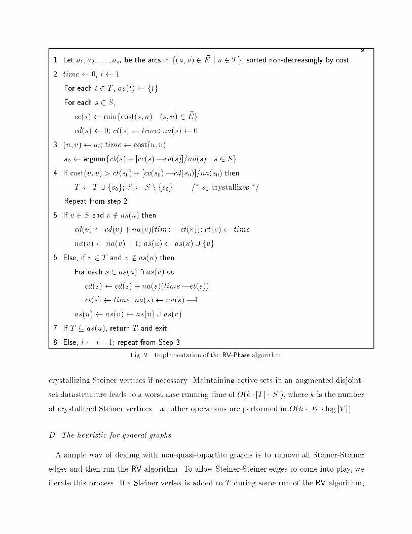
1. Let a1; a2; : : : ; am be the arcs in f(u; v) 2 ~E j u 2 Tg, sorted non-decreasingly by cost.
2. time 0, i 1
For each t 2 T , as(t) ftg
For each s 2 S,
cc(s) minfcost(s; u) j (s; u) 2 ~Eg
cd(s) 0; ct(s) time; na(s) 0
3. (u; v) ai; time cost(u; v)
s0 argminfct(s) + [cc(s)� cd(s)]=na(s) j s 2 Sg
4. If cost(u; v) > ct(s0) + [cc(s0)� cd(s0)]=na(s0) then
T T [ fs0g; S S n fs0g /* s0 crystallizes */
Repeat from step 2
5. If v 2 S and v =2 as(u) then
cd(v) cd(v) + na(v)(time� ct(v)); ct(v) time
na(v) na(v) + 1; as(u) as(u) [ fvg
6. Else, if v 2 T and v =2 as(u) then
For each s 2 as(u) \ as(v) do
cd(s) cd(s) + na(s)(time� ct(s))
ct(s) time; na(s) na(s)� 1
as(u) as(v) as(u) [ as(v)
7. If T � as(u), return T and exit.
8. Else, i i+ 1; repeat from Step 3.
Fig. 2. Implementation of the RV-Phase algorithm.
crystallizing Steiner vertices if necessary. Maintaining active sets in an augmented disjoint-
set datastructure leads to a worst case running time of O(k � jT j � jSj), where k is the number
of crystallized Steiner vertices|all other operations are performed in O(k � jEj � log jV j).
D. The heuristic for general graphs
A simple way of dealing with non-quasi-bipartite graphs is to remove all Steiner-Steiner
edges and then run the RV algorithm. To allow Steiner-Steiner edges to come into play, we
iterate this process. If a Steiner vertex is added to T during some run of the RV algorithm,
10
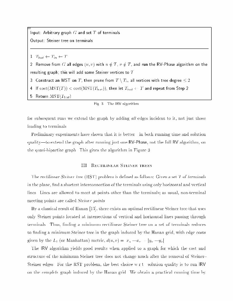
Input: Arbitrary graph G and set T of terminals.
Output: Steiner tree on terminals.
1. Tbest Tin T
2. Remove from G all edges (u; v) with u =2 T , v =2 T , and run the RV-Phase algorithm on the
resulting graph; this will add some Steiner vertices to T .
3. Construct an MST on T , then prune from T n Tin all vertices with tree degree � 2.
4. If cost(MST(T )) < cost(MST(Tbest)), then let Tbest T and repeat from Step 2.
5. Return MST(Tbest).
Fig. 3. The IRV algorithm.
for subsequent runs we extend the graph by adding all edges incident to it, not just those
leading to terminals.
Preliminary experiments have shown that it is better|in both running time and solution
quality|to extend the graph after running just one RV-Phase, not the full RV algorithm, on
the quasi-bipartite graph. This gives the algorithm in Figure 3.
III. Rectilinear Steiner trees
The rectilinear Steiner tree (RST) problem is de�ned as follows: Given a set T of terminals
in the plane, �nd a shortest interconnection of the terminals using only horizontal and vertical
lines. Lines are allowed to meet at points other than the terminals; as usual, non-terminal
meeting points are called Steiner points.
By a classical result of Hanan [13], there exists an optimal rectilinear Steiner tree that uses
only Steiner points located at intersections of vertical and horizontal lines passing through
terminals. Thus, �nding a minimum rectilinear Steiner tree on a set of terminals reduces
to �nding a minimum Steiner tree in the graph induced by the Hanan grid, with edge costs
given by the L1 (or Manhattan) metric, d(u; v) = jxu � xvj+ jyu � yvj.
The IRV algorithm yields good results when applied to a graph for which the cost and
structure of the minimum Steiner tree does not change much after the removal of Steiner-
Steiner edges. For the RST problem, the best choice w.r.t. solution quality is to run IRV
on the complete graph induced by the Hanan grid. We obtain a practical running time by
11applying a few simple, yet very e�ective, reductions to this graph.
A. Edge reductions
By a result of Robins and Salowe [23], for any set of points there exists a rectilinear MST
in which each point p has at most one neighbor in each of the four diagonal quadrants,
�x � y < x, �y < x � y, x < y � �x, and y � x < �y, translated at p. Hence,
the optimum Steiner tree in the quasi-bipartite graph is not a�ected if we remove all edges
incident to a Steiner vertex except those connecting it to the closest terminals from each
quadrant. We can also discard all edges connecting pairs of terminals except for the jT j � 1
edges in MST(T )|this merely amounts to a particular choice of breaking ties between
terminal-terminal edges during RV-Phase. Combined, these two edge reductions leave a
quasi-bipartite graph with O(jT j+ jSj) edges, as opposed to O(jT j � (jT j+ jSj)) without edge
reductions.
B. Vertex reductions
Zachariasen [31] noted that reductions based on structural properties of full Steiner com-
ponents, which play a crucial role for exact algorithms such as [5], [28], can also be used to
remove from the Hanan grid a large number of Steiner vertices without a�ecting the opti-
mum Steiner tree. Simpler versions of these reductions su�ce in our case, since we only want
to leave una�ected the optimum Steiner tree in the graph that results after the removal of
Steiner-Steiner edges.
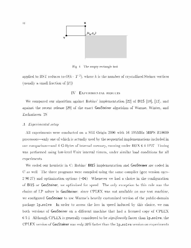
We incorporated in our code a version of the empty rectangle test [31], originally due
to Berman and Ramaiyer [2]. Consider a grid point found, say, at the intersection of the
vertical line through a terminal u and the horizontal line through a terminal v (see Figure 4).
The empty rectangle test says that the point must be retained in the graph only if (1) the
rectangle determined by terminals u and v is empty, i.e., contains no terminals in its interior,
and (2) the shaded quadrant contains at least one terminal. We used a simple O(jT j2)
implementation of this test; an O(jT j log jT j+ k) implementation, where k is the number of
empty rectangles, is also possible [9].
As noted in [6], [31], a stronger version of the empty rectangle test is guaranteed to remove
all but a set of O(jT j) Steiner points, still with no increase in the cost of the optimum RST
with no Steiner-Steiner edges. By using this stronger test the overall running time of IRV as
12
(x ,y )
v
u
u v
Fig. 4. The empty rectangle test.
applied to RST reduces to O(k � jT j2), where k is the number of crystallized Steiner vertices
(usually a small fraction of jT j).
IV. Experimental results
We compared our algorithm against Robins' implementation [22] of BI1S [18], [12], and
against the recent release [29] of the exact GeoSteiner algorithm of Warme, Winter, and
Zachariasen [28].
A. Experimental setup
All experiments were conducted on a SGI Origin 2000 with 16 195MHz MIPS R10000
processors|only one of which is actually used by the sequential implementations included in
our comparison|and 4 G-Bytes of internal memory, running under IRIX 6.4 IP27. Timing
was performed using low-level Unix interval timers, under similar load conditions for all
experiments.
We coded our heuristic in C; Robins' BI1S implementation and GeoSteiner are coded in
C as well. The three programs were compiled using the same compiler (gcc version egcs-
2.90.27) and optimization options (-O4). Whenever we had a choice in the con�guration
of BI1S or GeoSteiner, we optimized for speed. The only exception to this rule was the
choice of LP{solver in GeoSteiner: since CPLEX was not available on our test machine,
we con�gured GeoSteiner to use Warme's heavily customized version of the public-domain
package lp solve. In order to assess the loss in speed induced by this choice, we ran
both versions of GeoSteiner on a di�erent machine that had a licensed copy of CPLEX
6.5.1. Although CPLEX is generally considered to be signi�cantly faster than lp solve, the
CPLEX version of GeoSteiner was only 30% faster than the lp solve version on experiments
13involving 1000 random instances. We attribute the very competitive running time of the
lp solve version of GeoSteiner to code optimizations|made possible by intimate access to
the internals of lp solve|that are not included in the CPLEX version [27].
The test bed for our experiments consisted of two categories of instances:
� Random instances: For each instance size between 10 and 250, in increments of 10, we
generated uniformly at random 1,000 instances2 consisting of points in general position3
drawn from a 10000 � 10000 grid.
� Real VLSI instances: To further validate our results, we ran the three competing algo-
rithms on a set of 9 large instances extracted from two di�erent VLSI designs.
B. Solution quality
Following the standard practice [17], we use the percent improvement over the MST on
terminals,
cost(MST)� cost(Algo. RST)
cost(MST)� 100;
to compare the quality of the RSTs produced by the three algorithms.
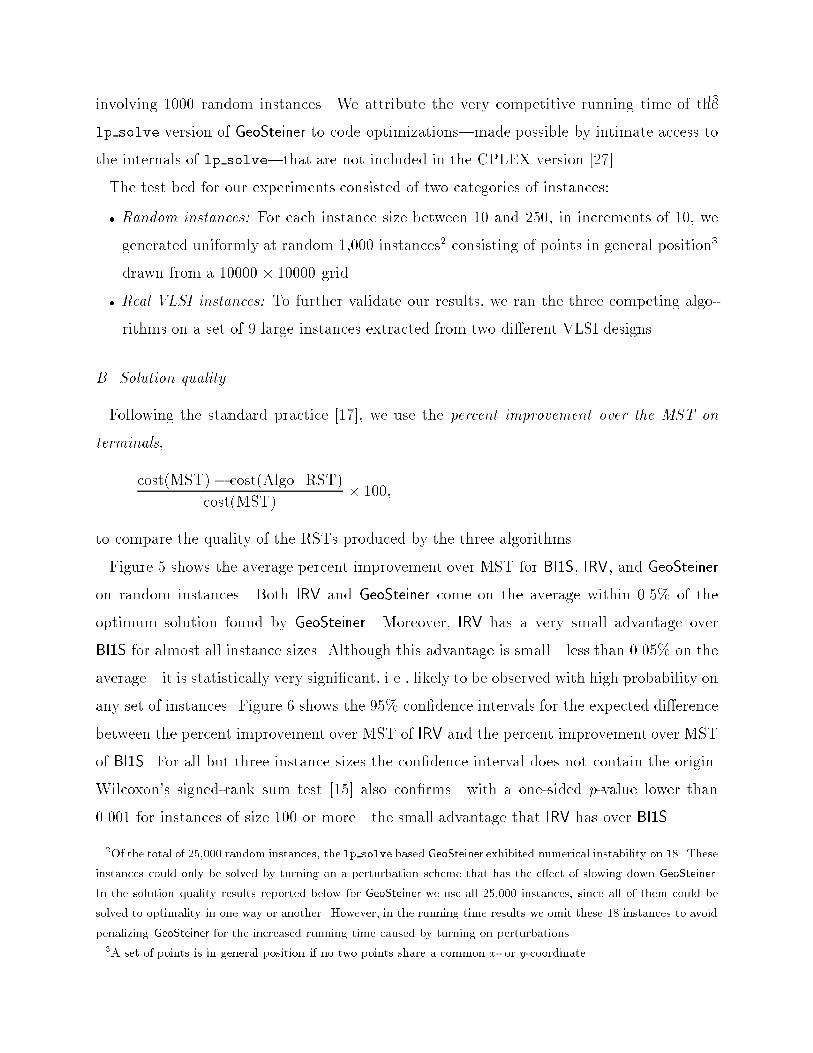
Figure 5 shows the average percent improvement over MST for BI1S, IRV, and GeoSteiner
on random instances. Both IRV and GeoSteiner come on the average within 0.5% of the
optimum solution found by GeoSteiner. Moreover, IRV has a very small advantage over
BI1S for almost all instance sizes. Although this advantage is small|less than 0.05% on the
average|it is statistically very signi�cant, i.e., likely to be observed with high probability on
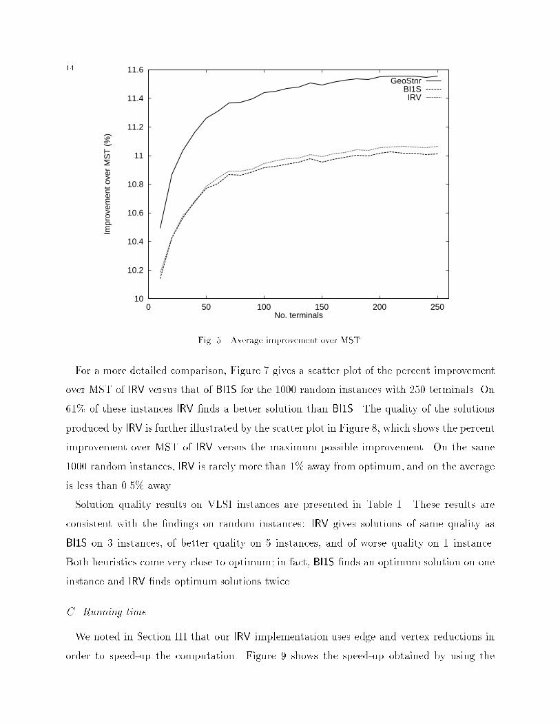
any set of instances. Figure 6 shows the 95% con�dence intervals for the expected di�erence
between the percent improvement over MST of IRV and the percent improvement over MST
of BI1S. For all but three instance sizes the con�dence interval does not contain the origin.
Wilcoxon's signed-rank sum test [15] also con�rms|with a one-sided p-value lower than
0.001 for instances of size 100 or more|the small advantage that IRV has over BI1S.
2Of the total of 25,000 random instances, the lp solve based GeoSteiner exhibited numerical instability on 18. These
instances could only be solved by turning on a perturbation scheme that has the e�ect of slowing down GeoSteiner.
In the solution quality results reported below for GeoSteiner we use all 25,000 instances, since all of them could be
solved to optimality in one way or another. However, in the running time results we omit these 18 instances to avoid
penalizing GeoSteiner for the increased running time caused by turning on perturbations.
3A set of points is in general position if no two points share a common x- or y-coordinate.
14
10
10.2
10.4
10.6
10.8
11
11.2
11.4
11.6
0 50 100 150 200 250
Impr
ovem
ent o
ver
MS
T (
%)
No. terminals
GeoStnrBI1SIRV
Fig. 5. Average improvement over MST.
For a more detailed comparison, Figure 7 gives a scatter plot of the percent improvement
over MST of IRV versus that of BI1S for the 1000 random instances with 250 terminals. On
61% of these instances IRV �nds a better solution than BI1S. The quality of the solutions
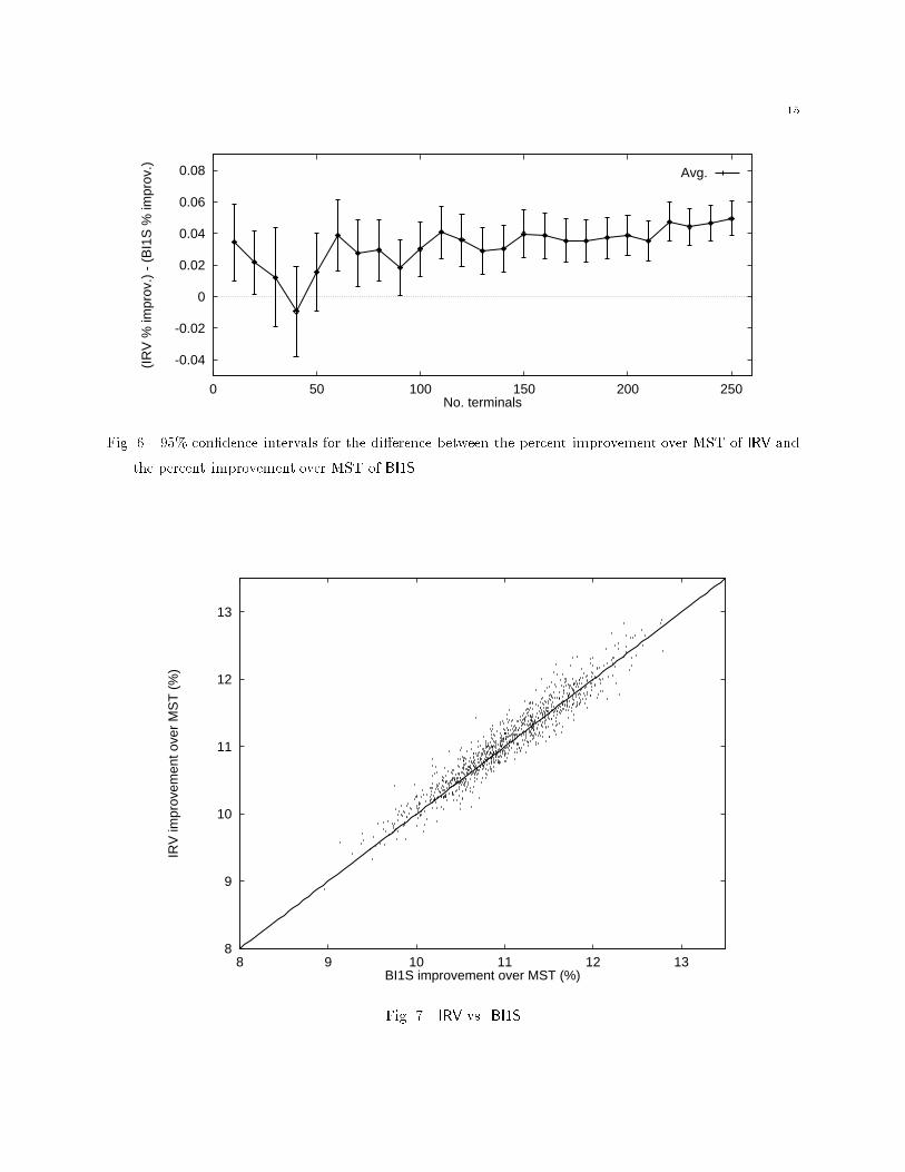
produced by IRV is further illustrated by the scatter plot in Figure 8, which shows the percent
improvement over MST of IRV versus the maximum possible improvement. On the same
1000 random instances, IRV is rarely more than 1% away from optimum, and on the average
is less than 0.5% away.
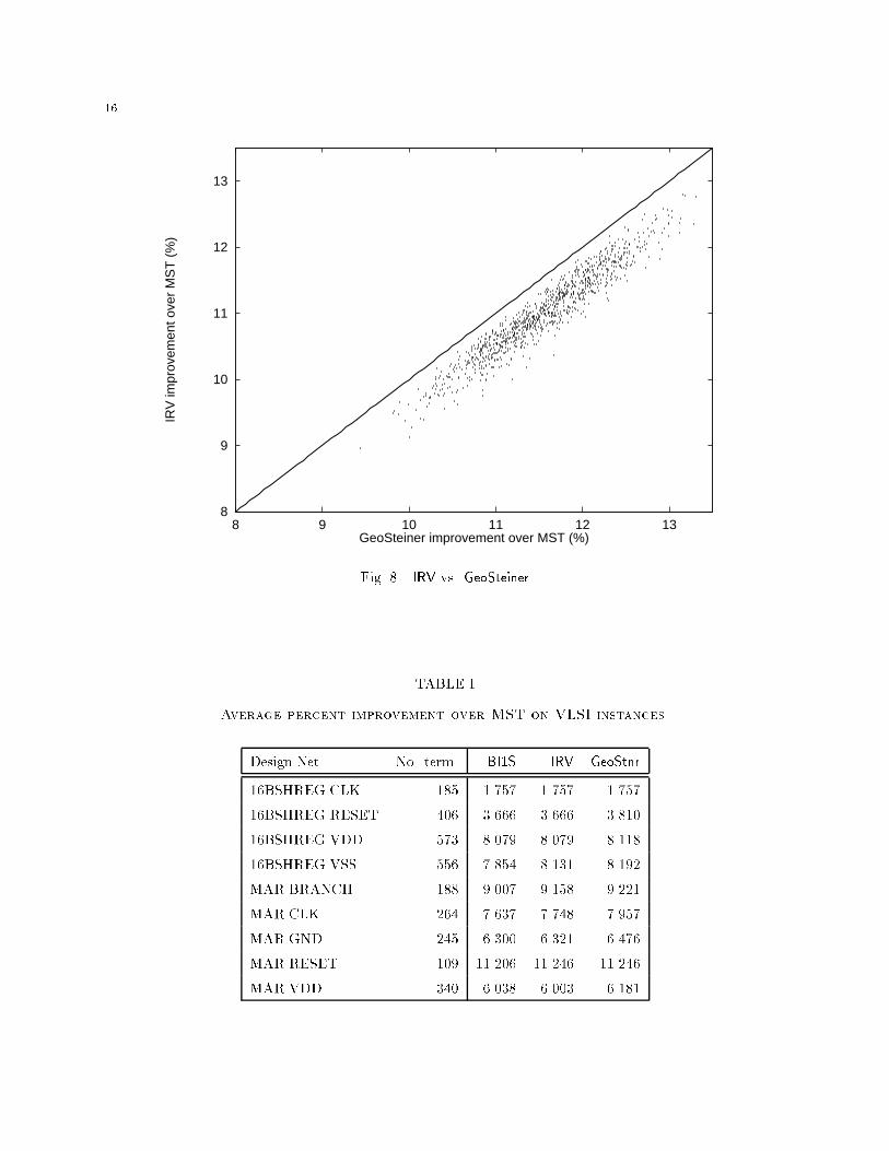
Solution quality results on VLSI instances are presented in Table I. These results are
consistent with the �ndings on random instances: IRV gives solutions of same quality as
BI1S on 3 instances, of better quality on 5 instances, and of worse quality on 1 instance.
Both heuristics come very close to optimum; in fact, BI1S �nds an optimum solution on one
instance and IRV �nds optimum solutions twice.
C. Running time
We noted in Section III that our IRV implementation uses edge and vertex reductions in
order to speed-up the computation. Figure 9 shows the speed-up obtained by using the
15
-0.04
-0.02
0
0.02
0.04
0.06
0.08
0 50 100 150 200 250
(IR
V %
impr
ov.)
- (
BI1
S %
impr
ov.)
No. terminals
Avg.
Fig. 6. 95% con�dence intervals for the di�erence between the percent improvement over MST of IRV and
the percent improvement over MST of BI1S.
8
9
10
11
12
13
8 9 10 11 12 13
IRV
impr
ovem
ent o
ver
MS
T (
%)
BI1S improvement over MST (%)
Fig. 7. IRV vs. BI1S
16
8
9
10
11
12
13
8 9 10 11 12 13
IRV
impr
ovem
ent o
ver
MS
T (
%)
GeoSteiner improvement over MST (%)
Fig. 8. IRV vs. GeoSteiner
TABLE I
Average percent improvement over MST on VLSI instances.
Design.Net No. term. BI1S IRV GeoStnr
16BSHREG.CLK 185 1.757 1.757 1.757
16BSHREG.RESET 406 3.666 3.666 3.810
16BSHREG.VDD 573 8.079 8.079 8.118
16BSHREG.VSS 556 7.854 8.131 8.192
MAR.BRANCH 188 9.007 9.158 9.221
MAR.CLK 264 7.637 7.748 7.957
MAR.GND 245 6.300 6.321 6.476
MAR.RESET 109 11.206 11.246 11.246
MAR.VDD 340 6.038 6.003 6.181
17
0
2
4
6
8
10
12
14
16
18
20
0 50 100 150 200 250
Spe
ed-u
p fa
ctor
No. terminals
Steiner pt. reductionBI1S speed-upIRV speed-up
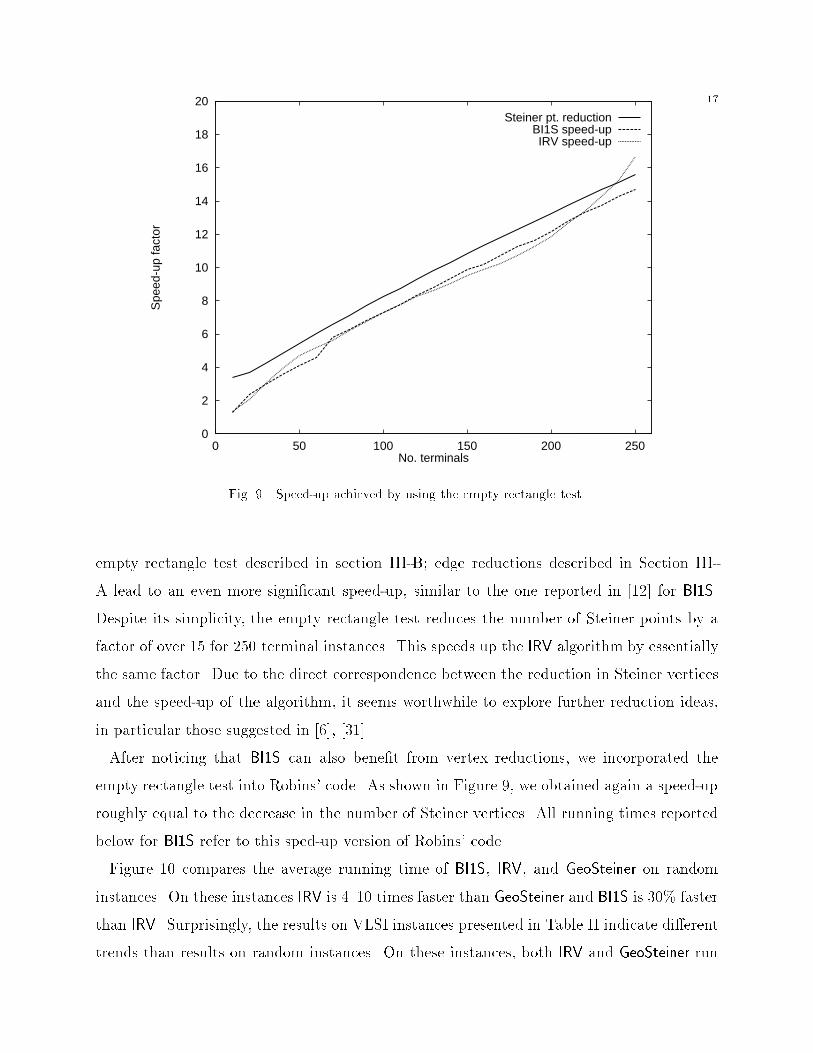
Fig. 9. Speed-up achieved by using the empty rectangle test.
empty rectangle test described in section III-B; edge reductions described in Section III-
A lead to an even more signi�cant speed-up, similar to the one reported in [12] for BI1S.
Despite its simplicity, the empty rectangle test reduces the number of Steiner points by a
factor of over 15 for 250 terminal instances. This speeds up the IRV algorithm by essentially
the same factor. Due to the direct correspondence between the reduction in Steiner vertices
and the speed-up of the algorithm, it seems worthwhile to explore further reduction ideas,
in particular those suggested in [6], [31].
After noticing that BI1S can also bene�t from vertex reductions, we incorporated the
empty rectangle test into Robins' code. As shown in Figure 9, we obtained again a speed-up
roughly equal to the decrease in the number of Steiner vertices. All running times reported
below for BI1S refer to this sped-up version of Robins' code.
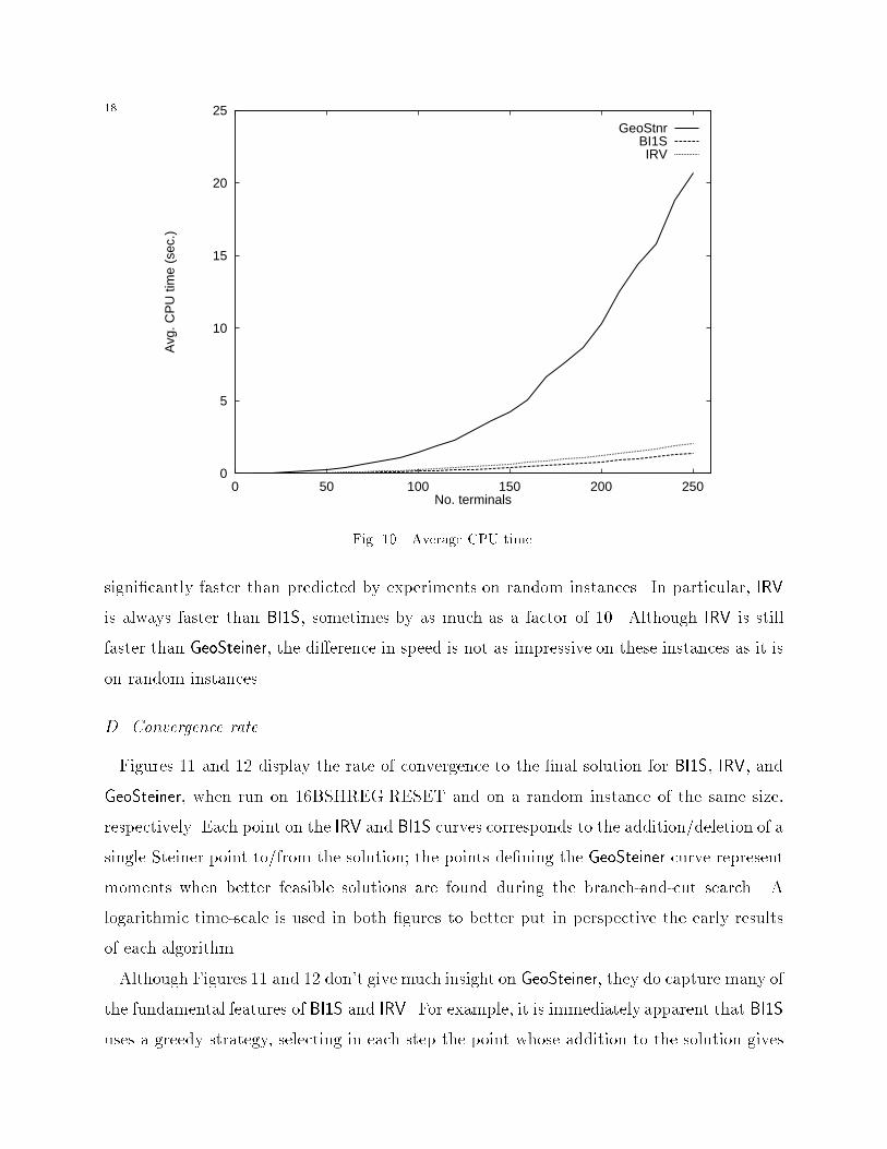
Figure 10 compares the average running time of BI1S, IRV, and GeoSteiner on random
instances. On these instances IRV is 4{10 times faster than GeoSteiner and BI1S is 30% faster
than IRV. Surprisingly, the results on VLSI instances presented in Table II indicate di�erent
trends than results on random instances. On these instances, both IRV and GeoSteiner run
18
0
5
10
15
20
25
0 50 100 150 200 250
Avg
. CP
U ti
me
(sec
.)
No. terminals
GeoStnrBI1SIRV
Fig. 10. Average CPU time.
signi�cantly faster than predicted by experiments on random instances. In particular, IRV
is always faster than BI1S, sometimes by as much as a factor of 10. Although IRV is still
faster than GeoSteiner, the di�erence in speed is not as impressive on these instances as it is
on random instances.
D. Convergence rate
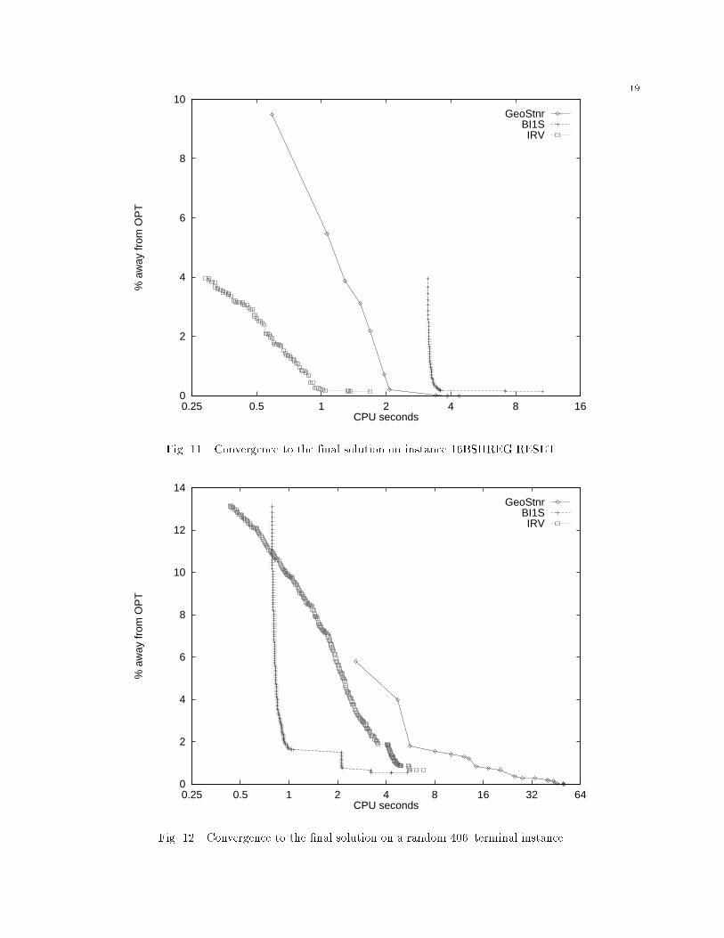
Figures 11 and 12 display the rate of convergence to the �nal solution for BI1S, IRV, and
GeoSteiner, when run on 16BSHREG.RESET and on a random instance of the same size,
respectively. Each point on the IRV and BI1S curves corresponds to the addition/deletion of a
single Steiner point to/from the solution; the points de�ning the GeoSteiner curve represent
moments when better feasible solutions are found during the branch-and-cut search. A
logarithmic time-scale is used in both �gures to better put in perspective the early results
of each algorithm.
Although Figures 11 and 12 don't give much insight on GeoSteiner, they do capture many of
the fundamental features of BI1S and IRV. For example, it is immediately apparent that BI1S
uses a greedy strategy, selecting in each step the point whose addition to the solution gives
19
0
2
4
6
8
10
0.25 0.5 1 2 4 8 16
% a
way
from
OP
T
CPU seconds
GeoStnrBI1SIRV
Fig. 11. Convergence to the �nal solution on instance 16BSHREG.RESET.
0
2
4
6
8
10
12
14
0.25 0.5 1 2 4 8 16 32 64
% a
way
from
OP
T
CPU seconds
GeoStnrBI1SIRV
Fig. 12. Convergence to the �nal solution on a random 406{terminal instance.
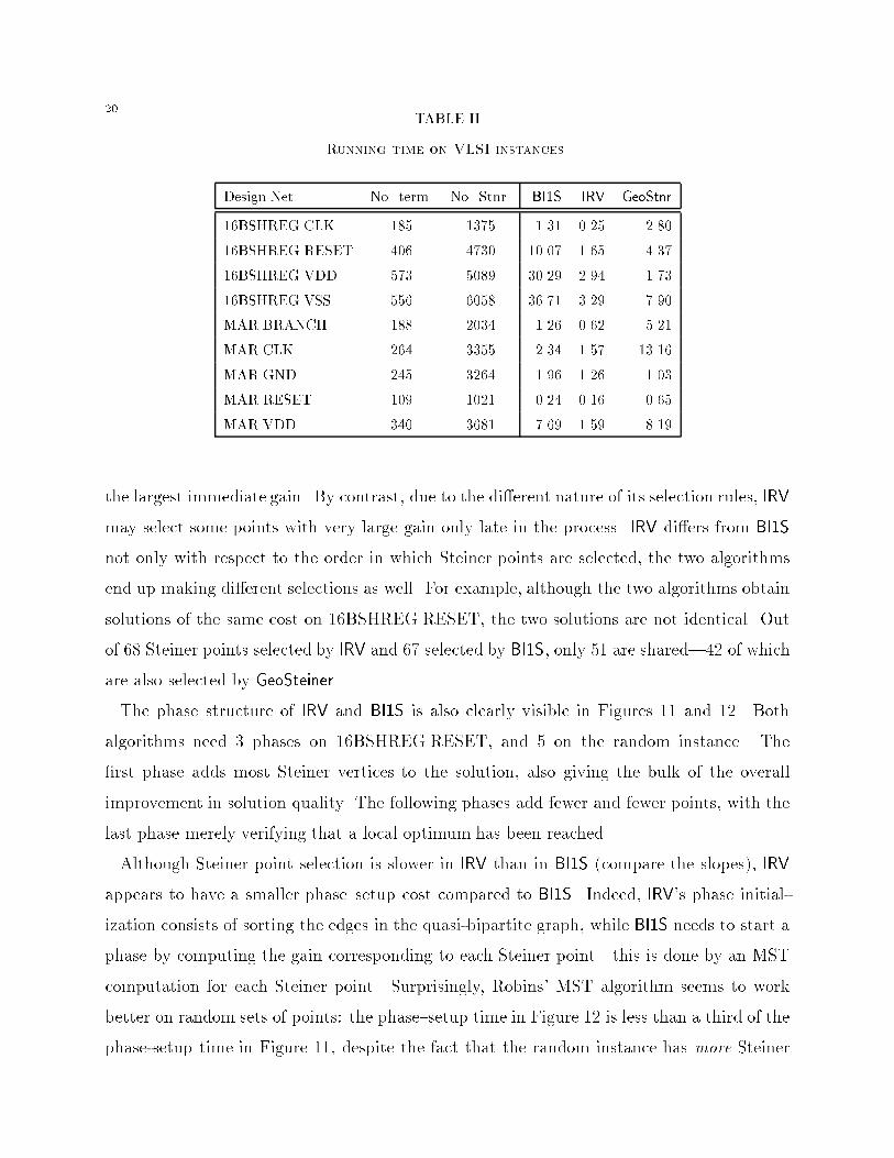
20TABLE II
Running time on VLSI instances.
Design.Net No. term. No. Stnr. BI1S IRV GeoStnr
16BSHREG.CLK 185 1375 1.31 0.25 2.80
16BSHREG.RESET 406 4730 10.07 1.65 4.37
16BSHREG.VDD 573 5089 30.29 2.94 1.73
16BSHREG.VSS 556 6058 36.71 3.29 7.90
MAR.BRANCH 188 2034 1.26 0.62 5.21
MAR.CLK 264 3355 2.34 1.57 13.16
MAR.GND 245 3264 1.96 1.26 1.03
MAR.RESET 109 1021 0.24 0.16 0.65
MAR.VDD 340 3681 7.69 1.59 8.19
the largest immediate gain. By contrast, due to the di�erent nature of its selection rules, IRV
may select some points with very large gain only late in the process. IRV di�ers from BI1S
not only with respect to the order in which Steiner points are selected, the two algorithms
end up making di�erent selections as well. For example, although the two algorithms obtain
solutions of the same cost on 16BSHREG.RESET, the two solutions are not identical. Out
of 68 Steiner points selected by IRV and 67 selected by BI1S, only 51 are shared|42 of which
are also selected by GeoSteiner.
The phase structure of IRV and BI1S is also clearly visible in Figures 11 and 12. Both
algorithms need 3 phases on 16BSHREG.RESET, and 5 on the random instance. The
�rst phase adds most Steiner vertices to the solution, also giving the bulk of the overall
improvement in solution quality. The following phases add fewer and fewer points, with the
last phase merely verifying that a local optimum has been reached.
Although Steiner point selection is slower in IRV than in BI1S (compare the slopes), IRV
appears to have a smaller phase{setup cost compared to BI1S. Indeed, IRV's phase initial-
ization consists of sorting the edges in the quasi-bipartite graph, while BI1S needs to start a
phase by computing the gain corresponding to each Steiner point|this is done by an MST
computation for each Steiner point. Surprisingly, Robins' MST algorithm seems to work
better on random sets of points: the phase{setup time in Figure 12 is less than a third of the
phase-setup time in Figure 11, despite the fact that the random instance has more Steiner
21points (7366 versus 4730 in 16BSHREG.RESET). This explains why BI1S is faster than IRV
on random instances but not on VLSI instances.
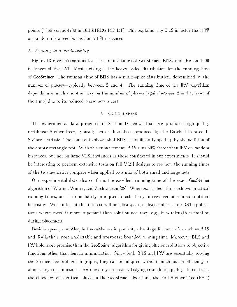
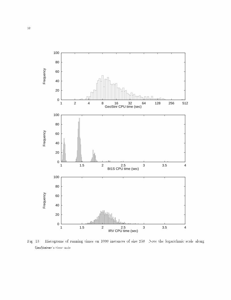
E. Running time predictability
Figure 13 gives histograms for the running times of GeoSteiner, BI1S, and IRV on 1000
instances of size 250. Most striking is the heavy{tailed distribution for the running time
of GeoSteiner. The running time of BI1S has a multi-spike distribution, determined by the
number of phases|typically between 2 and 4. The running time of the IRV algorithm
depends in a much smoother way on the number of phases (again between 2 and 4, most of
the time) due to its reduced phase{setup cost.
V. Conclusions
The experimental data presented in Section IV shows that IRV produces high-quality
rectilinear Steiner trees, typically better than those produced by the Batched Iterated 1-
Steiner heuristic. The same data shows that BI1S is signi�cantly sped up by the addition of
the empty rectangle test. With this enhancement, BI1S runs 30% faster than IRV on random
instances, but not on large VLSI instances as those considered in our experiments. It should
be interesting to perform extensive tests on full VLSI designs to see how the running times
of the two heuristics compare when applied to a mix of both small and large nets.
Our experimental data also con�rms the excellent running time of the exact GeoSteiner
algorithm of Warme, Winter, and Zachariasen [28]. When exact algorithms achieve practical
running times, one is immediately prompted to ask if any interest remains in sub-optimal
heuristics. We think that this interest will not disappear, at least not in those RST applica-
tions where speed is more important than solution accuracy, e.g., in wirelength estimation
during placement.
Besides speed, a subtler, but nonetheless important, advantage for heuristics such as BI1S
and IRV is their more predictable and worst-case bounded running time. Moreover, BI1S and
IRV hold more promise than the GeoSteiner algorithm for giving e�cient solutions to objective
functions other than length minimization. Since both BI1S and IRV are essentially solving
the Steiner tree problem in graphs, they can be adapted without much loss in e�ciency to
almost any cost function|IRV does rely on costs satisfying triangle inequality. In contrast,
the e�ciency of a critical phase in the GeoSteiner algorithm, the Full Steiner Tree (FST)
22
0
20
40
60
80
100
1 2 4 8 16 32 64 128 256 512
Fre
quen
cy
GeoStnr CPU time (sec)
0
20
40
60
80
100
1 1.5 2 2.5 3 3.5 4
Fre
quen
cy
BI1S CPU time (sec)
0
20
40
60
80
100
1 1.5 2 2.5 3 3.5 4
Fre
quen
cy
IRV CPU time (sec)
Fig. 13. Histograms of running times on 1000 instances of size 250. Note the logarithmic scale along
GeoSteiner's time axis.
23generation phase, heavily depends on structural properties speci�c to the underlying metric
space. Even when well-understood, these structural properties may not lead to the same
e�ciency as in the rectilinear case. For example, FST generation is more than 100 times
slower on Euclidean instances than it is on rectilinear ones, and becomes in this case the
bottleneck of the whole algorithm [28].
VI. Acknowledgments
The authors wish to thank Sridhar Rajagopalan for his involvement with an earlier version
of this work, Alex Zelikovsky for many enlightening discussions, and one of the anonymous
referees for many constructive comments that helped improving the presentation.
References
[1] A. Agrawal, P. Klein, and R. Ravi. When trees collide: An approximation algorithm for the generalized Steiner
problem on networks, SIAM J. on Computing, 24 (1995), pp. 440{456.
[2] P. Berman and V. Ramaiyer. Improved approximations for the Steiner tree problem, J. of Algorithms, 17 (1994),
pp. 381{408.
[3] M. Borah, R.M. Owens, and M.J. Irwin. An edge-based heuristic for Steiner routing, IEEE Trans. on CAD 13
(1994), pp. 1563{1568.
[4] T.H. Cormen, C.E. Leiserson, and R.L. Rivest. Introduction to algorithms, MIT Press, Cambridge, MA, 1990.
[5] U. F�ossmeier and M. Kaufmann. Solving rectilinear Steiner tree problems exactly in theory and practice, Proc.
5th European Symp. on Algorithms (1997), Springer-Verlag LNCS 1284, pp. 171{185.
[6] U. F�ossmeier, M. Kaufmann, and A. Zelikovsky. Faster approximation algorithms for the rectilinear Steiner tree
problem, Discrete and Computational Geometry 18 (1997), pp. 93{109.
[7] J.L. Ganley. Computing optimal rectilinear Steiner trees: A survey and experimental evaluation, Discrete Applied
Mathematics, 89 (1998), pp. 161{171.
[8] J.L. Ganley and J.P. Cohoon. Improved computation of optimal rectilinear Steiner minimal trees, Int. J. of
Computational Geometry and Applications, 7 (1997), pp. 457{472.
[9] R.-H, G�uting, O. Nurmi, and T. Ottmann. Fast algorithms for direct enclosures and direct dominances, J. of
Algorithms, 10 (1989), pp. 170{186.
[10] M.R. Garey and D.S. Johnson. The rectilinear Steiner tree problem is NP-complete, SIAM J. Appl. Math., 32
(1977), pp. 826{834.
[11] M.X. Goemans and D.P. Williamson. A general approximation technique for constrained forest problems, SIAM
J. on Computing, 24 (1995), pp. 296{317.
[12] J. Gri�th, G. Robins, J.S. Salowe, and T. Zhang. Closing the gap: near-optimal Steiner trees in polynomial
time, IEEE Trans. on CAD, 13 (1994), pp. 1351{1365.
[13] M. Hanan. On Steiner's problem with rectilinear distance, SIAM J. Appl. Math., 14 (1966), pp. 255{265.
[14] J.-M. Ho, G. Vijayan, and C.K. Wong. New algorithms for the rectilinear Steiner tree problem, IEEE Trans. on
CAD, 9 (1990), pp. 185{193.
[15] M. Hollander and D.A. Wolfe. Nonparametric Statistical Methods, 2nd Edition, John Wiley & Sons, 1999.
24[16] F.K. Hwang. An O(n log n) algorithm for suboptimal rectilinear Steiner trees, IEEE Trans. on Circuits and
Systems, 26 (1979), pp. 75{77.
[17] F.K. Hwang, D.S. Richards, and P. Winter. The Steiner tree problem, Ann. of Discrete Math. 53, North-Holland,
Amsterdam, 1992.
[18] A.B. Kahng and G. Robins. A new class of iterative Steiner tree heuristics with good performance, IEEE Trans.
on CAD, 11 (1992), pp. 1462{1465.
[19] F.D. Lewis, W.C.-C. Pong, and N. Van Cleave. Local improvement in Steiner trees, Proc. of the 3rd Great Lakes
Symp. on VLSI (1993), pp. 105{106.
[20] H. J. Pr�omel and A. Steger. RNC-approximation algorithms for the Steiner problem, in R. Reischuk and M. Mor-
van, editors, Proc. of the 14th Symp. on Theoretical Aspects of Computer Science (1997), volume 1200 of Lecture
Notes in Computer Science, pages 559{570.
[21] S. Rajagopalan and V.V. Vazirani. On the bidirected cut relaxation for the metric Steiner tree problem, 10th
ACM-SIAM Symp. on Discrete Algorithms, 1999, pp. 742{751.
[22] G. Robins. Steiner code available at
www.cs.virginia.edu/~robins/steiner.tar.
[23] G. Robins and J.S. Salowe. Low-degree minimum spanning trees, Discrete and Computational Geometry 14
(1995), pp. 151{165.
[24] G. Robins and A. Zelikovsky. Improved Steiner Tree Approximation in Graphs, to appear in Proc. of ACM/SIAM
Symposium on Discrete Algorithms (SODA'2000).
[25] J.S. Salowe and M.D. Warme. Thirty-�ve-point rectilinear Steiner minimal trees in a day, Networks 25 (1995),
pp. 69{87.
[26] V.V. Vazirani. Approximation Algorithms. Book in preparation available at
www.cc.gatech.edu/fac/Vijay.Vazirani/book.ps.
[27] D.M. Warme. E-mail communication, September 1999.
[28] D.M. Warme, P. Winter, and M. Zacharisen. Exact Algorithms for Plane Steiner Tree Problems: A Computa-
tional Study, Technical Report DIKU-TR-98/11, Dept. of Computer Science, University of Copenhagen, 1998.
[29] D.M. Warme, P. Winter, and M. Zacharisen. GeoSteiner 3.0 package, available at
ftp.diku.dk/diku/users/martinz/geosteiner-3.0.tar.gz.
[30] Y.F. Wu, P. Widmayer, and C.K. Wong. A faster approximation algorithm for the Steiner problem in graphs,
Algorithmica 23 (1986), pp. 223{229.
[31] M. Zachariasen. Rectilinear Full Steiner Tree Generation, Networks 33 (1999), pp. 125{143.
[32] A. Zelikovsky. An 11/6-approximation algorithm for the network Steiner problem, Algorithmica, 9 (1993), pp
463{470.


