27
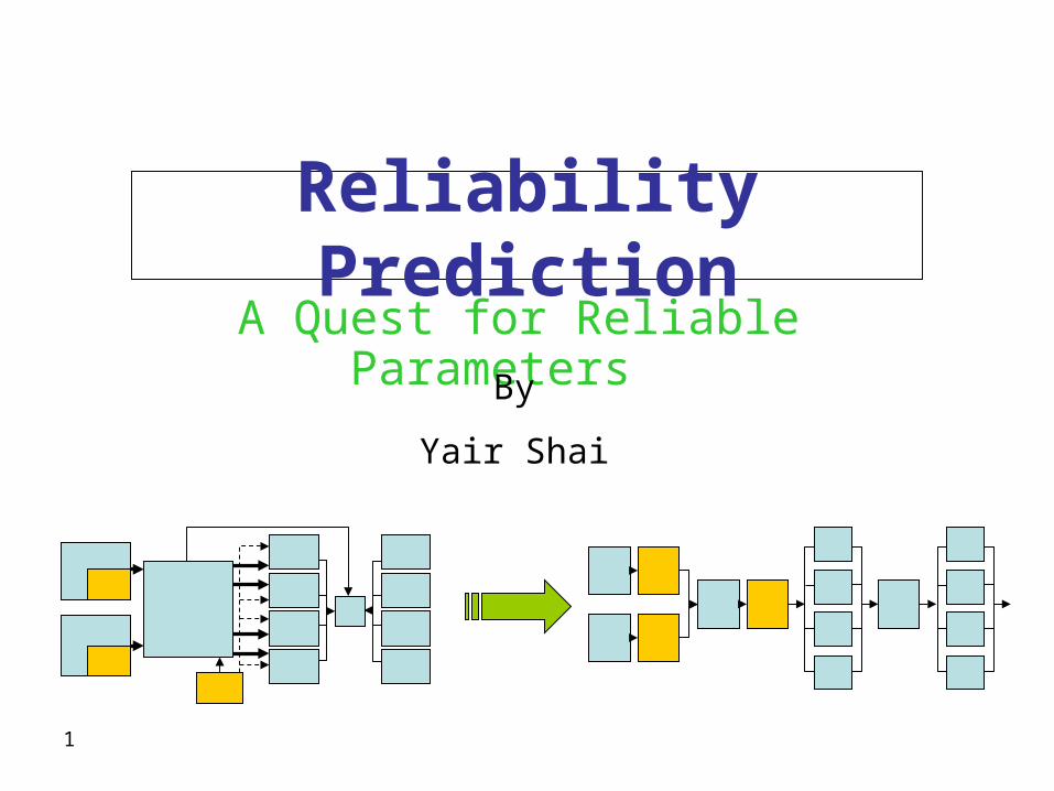
1 Reliability Prediction A Quest for Reliable Parameters By Yair Shai
| Date post: | 25-Dec-2015 |
| Category: |
Documents |
| Upload: | sharyl-heath |
| View: | 221 times |
| Download: | 0 times |
1
Reliability PredictionA Quest for Reliable Parameters
By
Yair Shai

2
Goals
• Compare the MTBCF & MTTCF parameters in view of complex systems engineering.
• Failure repair policy as the backbone for realistic MTBCF calculation.
• Motivation for modification of the technical specification requirements.

3
Promo : Description of Parameters
r
ti
i
timet1 t2 t3 t4 t5 .......
Failure Event of an Item
Repairable Items:
Mean Time Between Failures =
Non Repairable Items:
Mean Time To Failure =
r
ti
ir =Number of Failures
Seman
tics
?

4
MTBF = MTTF?? An assumption:
Failed item returns to “As Good As New” status after repair or renewal.
note: Time To Repair is not considered.
UP
DOWN
TIME

5
Critical FailuresMoving towards System Design
A System Failure resulting in (temporary or permanent) Mission Termination.
COMPUTER
COMPUTER
SUBSYSTEM
A simple configuration of parallel hot Redundancy.
A Failure: any computer failure
A Critical Failure: two computers failed
XX

6
Critical FailuresA clue for Design Architecture
MTBCF
Mean Time Between Critical Failures
MTTCF
Mean Time To Critical Failure
SAME? Remember the assumptions
Determining the failure repair policy: COLD REPAIR
No time for repair actions during the mission

7
Functional System Design
Operational Demand: At least two receiver units and one antenna should work to operate the system.
CPU
CPUPOWER
SUPPLY
POWER SUPPLY 4 CHANNEL
RECEVERCONTROLER
UNIT A
UNIT B
UNIT C
UNIT D
POWER SUPPLY
ANTENA
ANTENA
ANTENA
ANTENA
2 / 4
sw
Switch control

8
From System Design to Reliability Model
Serial model : Rs = R1x R2
Parallel model : Rs = 1- (1-R1)x(1-R2)
K out of N model : Rs = Binomial Solution
CPU PS1
CPU PS1
CONT PS2
A
B
C
D
2 / 4
xx
x
ANT
ANT
ANT
ANT
sw
Is this a Critical Failure ?
INDEPENDENT
BLOCKS
9
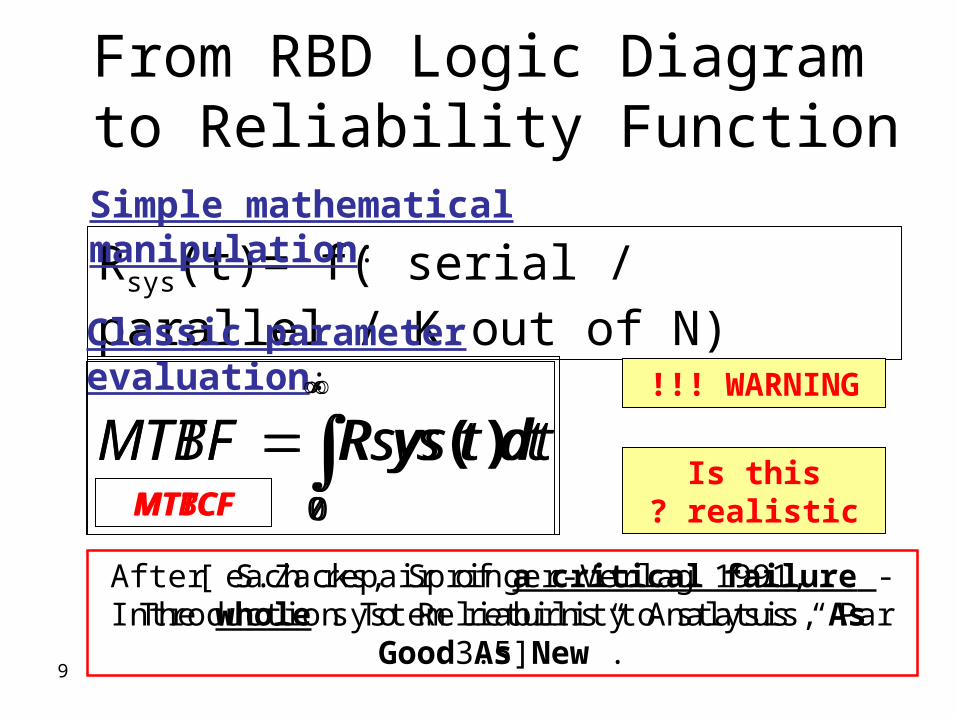
From RBD Logic Diagram to Reliability Function
Rsys(t)= f( serial / parallel / K out of N)Classic parameter evaluation:
0
)( dttRsysMTBFWARNING!!!
After each repair of a critical failure - The whole system returns to status “As Good As New”.
Is this realistic?
Simple mathematical manipulation:
MTTCF 0
( )MTTF Rsys t dt
MTBCF
[ S.Zacks, Springer-Verlag 1991, Introduction To Reliability Analysis, Par 3.5]

10
Realistic interpretation:
MTBCF = MTTCF
Only failed Items which cause the failure are repaired to idle. All other components keep on aging.
MTBCF vs. MTTCFA New Interpretation
Common practice interpretation:
MTBCF = MTTCF = MTTCFF
Each repair “Resets” the time count to idle status (or) Each failure is the first failure.
First

11
Presentation I
TTCF
23
1
231
3 12
1
231
2
A B CHAD WE KNOWN
THE FUTURE…
Simple 3 aging components serial system model
AB
C

12
Presentation IISimple 3 aging components serial system model
A B C
TBCF
11
1
32
2
323
4
HAD WE KNOWN
THE FUTURE…
4 AB
C

13
Presentation III Simple 3 aging components serial system model
A B C
AB
C
TBCF
11
1
32
2
323
4
AB
C
TTCF
23
1
231
3 12
HAD WE KNOWN
THE FUTURE…
1
4
231
2
MTBCF < MTTCF

14
Simulation MethodMONTE – CARLO
MATHCAD
N=
100,
000
SE
TS
MIN (X1,1 X2,1 X3,1)
MIN (X1,2 X2,2 X3,2)
.……
……
……
……
MIN (X1,N X2,N X3,N)_________________
N
iiN 1
min1
N=
100,
000
SE
TS
MIN (X1,1 X2,1 X3,1)
MIN (X1,2 Δ1,2 Δ2,2)
.……
……
……
……
MIN (X1,N Δ1,N Δ2,N)_________________
N
iiN 1
min1

15
How “BIG” is the Difference?
1. Depends on the System Architecture.
2. Depends on the Time-To-Failure distribution of each component.
3. The difference in a specific complex electronic system was found to be ~40%
Note: True in redundant systems even when all components have constant failure rates.

16
Why Does It Matter? Suppose a specification demand for a system’s reliability :
MTBCF = 600 hour
Suppose the manufacturer prediction of the parameter:
MTBCF = 780 hour
ATTENTION !!! How was it CALCULATED ????
Is this MTBCF or MTTCF ????
X -40%
“Real” MTBCF = 480 < 600 (spec)

17
Example 1
Aging serial system – each component is weibull distributed

18
התפלגות ווייבול זהה לכל הפריטים

19
התפלגות ווייבול זהה לכל הפריטים

20
התפלגות ווייבול זהה לכל הפריטים

21
התפלגות ווייבול זהה לכל הפריטים

22
Example 2Two redundant subsystems in series –
each component is exponentially distributed
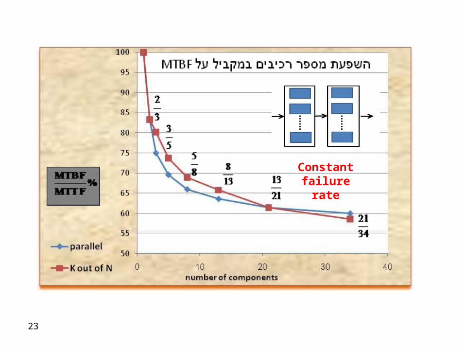
23
Constant failure rate

24
serial
parallel
Constant failure rate
25
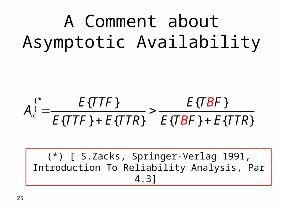
A Comment about Asymptotic Availability
{ } { }
{ } { } { } { }
E TTF E T FA
E TTF E TTR E T F E
B
B TTR
(*)
(*) [ S.Zacks, Springer-Verlag 1991, Introduction To Reliability Analysis, Par 4.3]

26
Repair policies
1. “Hot repair” is allowed for redundant components.
2. All components are renewed on every failure event.
3. All failed components are renewed on every failure event.
4. Failed components are renewed only in blocks which caused the system failure.
5. Failed subsystems are only partially renewed.

27
Conclusions
• System configuration and distribution of components determine the gap.
• Repair policy should be specified in advance to determine calculation method.
• Flexible software solutions are needed to simulate real MTBCF for a given RBD.
• Predict MTBCF not MTTCF


