1 s2.0-s0141118799000115-main

Deterministic wave model for short-crested ocean waves:Part I. Theory and numerical scheme

J. Zhang*, J. Yang, J. Wen, I. Prislin, K. Hong

Ocean Engineering Program, Department of Civil Engineering, Texas A&M University, College Station, TX 77843-3136, USA

Received 26 October 1998; received in revised form 15 March 1999; accepted 22 March 1999

Abstract

A directional hybrid wave model (DHWM) has been developed for deterministic prediction of short-crested irregular ocean waves. Inusing the DHWM, a measured wave field is first decomposed into its free-wave components based on as few as three point measurements.Then the wave properties are predicted in the vicinity of the measurements based on the decomposed free-wave components. Effects ofnonlinear interactions among the free-wave components up to second order in wave steepness are considered in both decomposition andprediction. While the prediction scheme is straightforward, the decomposition scheme is innovative and accomplished through an iterativeprocess involving three major steps. The extended maximum likelihood method is employed to determine the directional wave spreading; theinitial phases of directional free-wave components are determined using a least-square fitting scheme; and nonlinear effects are computedusing both conventional and phase modulation methods to achieve fast convergence. The free-wave components are obtained after thenonlinear effects being decoupled from the measurements. Variety of numerical tests have been conducted, indicating that the DHWM isconvergent and reliable.q 1999 Elsevier Science Ltd. All rights reserved.

Keywords:Short-crested ocean waves; Directional hybrid wave model; Second-order nonlinear interactions

1. Introduction

A deterministic description of directional waves canprovide the prediction of wave properties in the time domainbased on related measurements. This capability is not avail-able in existing studies, and yet is highly desirable to manyocean and coastal science and engineering applications. Forexample, in order to determine the statistics of typical waveproperties of rough seas, such as wave groupiness, the maxi-mum wave height, crest height and related wave period,measured surface elevations are needed. While surfaceelevations can be readily measured in the laboratory, surfaceelevations in the ocean are often indirectly measured usingpressure transducers, velocity meters or other instruments. Itrequires the capability of deducing the surface elevationbased on indirect measurements. This study aims at thedevelopment of a nonlinear directional wave model whichcan make the deterministic predictions of general waveproperties of short-crested seas based on the measurementsof a variety of commonly deployed instruments.

Ocean waves are viewed as the constitution of many

wave components of different frequencies and amplitudes,and advancing in different directions. The basic wavecomponents, known as free-wave (or linear) components,obey the dispersion relation. Due to the nonlinear natureof surface waves, the interactions among these free-wavecomponents result in bound-wave components which do notobey the dispersion relation. When linear wave theory isemployed, bound-wave components are either ignored ortreated as if they were free-wave components. In general,the procedures of predicting wave properties are first todecompose a measured wave field into free-wave compo-nents and then to superpose the wave properties of the free-wave components and their interactions (bound-wavecomponents). In the case of unidirectional irregular waves,linear wave theory together with the Fast Fourier Transform(FFT) can deterministically predict wave properties basedon a point measurement. In the case of directional seas, thenumber of simultaneous wave records of a wave field isoften limited to as few as three to five due to the costs. Asa result, the use of two-dimensional FFT to decompose awave field is no longer applicable. Alternatively, linearwave theory together with cross-spectrum analyses areused to derive a directional frequency-amplitude or energyspectrum but the information of the initial phases of wavecomponents is not retained. Quite different from

Applied Ocean Research 21 (1999) 167–188

0141-1187/99/$ - see front matterq 1999 Elsevier Science Ltd. All rights reserved.PII: S0141-1187(99)00011-5

www.elsevier.com/locate/apor

* Corresponding author. Tel.:1 1-409-845-4515; fax:1 1-409-862-8162.

E-mail address:[email protected] (J. Zhang)

unidirectional waves, wave properties of short-crestedocean waves in general cannot be deterministicallypredicted based on the measurements even within thescope of linear wave theory. Wave properties are simulatedbased on the assumption of random initial phases. It is wellknown that quite different wave processes may have thesame or similar spectrum if the relative phases of wavecomponents are not specified [1].

In steep ocean waves, the contributions of bound-wavecomponents may become dominant or important withrespect to the free-wave components of the same frequencyin the frequency bands either lower or higher than the spec-tral peak frequency [2]. Because the relationship betweenthe elevation and potential amplitudes of a free-wavecomponent is different from that of a bound-wave compo-nent of the same frequency, predicted wave properties usinglinear wave theory, for example, wave kinematics based onmeasured wave elevation or wave elevation based onmeasured dynamic pressure, were found to be quite inaccu-rate for steep waves. [3–5]. For accurate prediction,nonlinear wave effects have to be considered in the decom-position as well as superposition of a wave field. That is, thebound-wave components are decoupled from the measuredwave characteristics before a wave field is decomposed intoits free-wave components. Based on the free-wave compo-nents, the bound-wave components can be computed andthe resultant wave properties nearby the measurementscan be obtained as the superposition of free-wave andbound-wave components. In the case of unidirectional irre-gular waves, it has been shown that the approach mentionedabove, named as the hybrid nonlinear wave model (HWM),can provide more accurate predictions than linear wavetheory [4]. Encouraged by that success, this study is envi-sioned.

Due to the limitation on the measurements of short-crested waves, previous studies have been overwhelminglydominated by statistical approaches. The statisticalapproaches based on linear wave theory were well docu-mented [6]. Using weakly nonlinear wave theory, attemptswere made to decouple the energy of bound-wave compo-nents from the measured energy spectrum [7–9]. Assuminga directional wave-energy spreading function, Masuda et al.[10] and Mitsuyasu et al. [11] showed that the contributionfrom second order bound-wave components on phase velo-city is significant in wind waves generated in a flume. Usingpoly-spectra analyses, Herbers and Guza [12,13] showedthat the nonlinear contributions from the sum- and differ-ence-frequency interactions could be significant inmeasured short-crested wave pressure and particle veloci-ties. In spite of many differences, a common assumptionmade in these studies is that the initial phases of free-wave components are independent and randomly distributedbetween 0 and 2p. Contrary to the abundant studies usingstatistical approaches, the studies using deterministicapproaches were very rare. Our literature survey onlyfound an early attempt by Sand [14] and recent one by

Schaffer and Hyllested [15], and both of them werebased on linear wave theory. Besides, their methods werelimited to the measurements of one surface elevation andtwo horizontal velocity components and sometimesthere could be significant energy losses during the wavedecomposition.

A directional hybrid wave model (DHWM) is determi-nistic and considers both wave directionality and nonlinear-ity. In several respects, the model is unique. First, based onas few as three measurements recorded at fixed-points, theDHWM decouples nonlinear effects from the measurementsand then decomposes the measured directional irregularwave field into free-wave components without the assump-tions of random initial phases of free-wave components anda prior directional spreading function. Secondly, thenonlinear effects are calculated by using two differentperturbation approaches: a conventional and a phase modu-lation methods. It was found that truncated solutions forbound-wave components given by a conventional perturba-tion method may not converge if the wavelengths of twointeracting wave components are quite different while theconvergent solutions can be obtained using the phase modu-lation method [16]. For a wave field of energy distributed ina relatively broad frequency range, the use of both conven-tional and phase modulation methods to describe the wave–wave interaction can provide convergent solutions forunidirectional irregular waves [2], which will also benumerically demonstrated for multi-directional waves inSection 6.1. In our earlier study, only conventional methodwas used for the solution of bound-wave components, whichlimits the application to a wave field of a relatively narrow-band spectrum [17]. Thirdly, the model renders determinis-tic predictions of wave characteristics of a measured direc-tional field. A variety of wave measurements (pressuretransducers, surface piercing wave gauges and velocimetry)can be used as input for the wave decomposition. Since allwave properties can be computed based on the potential offree-wave components, the DHWM can be straightfor-wardly extended to allow for other measurements, such aswave slopes and accelerations as well. Finally, because ofabove capabilities, extensive and rigorous examinationsabout the validity and accuracy of this model can be madethrough the comparisons in the time-domain between thepredictions and the corresponding laboratory and fieldmeasurements.

In addition to the neglect of viscosity, wind effects, andwave breaking, the current DHWM is truncated at secondorder in wave steepness. The ‘weak’ or resonant wave inter-actions in deep or intermediate-depth water are of thirdorder and hence are not considered. The weak wave inter-actions can become substantial after hundreds of dominantwave periods [18,19]. Hence, for accurate prediction, thecomputation of wave properties based on this study shouldbe limited within a short distance from the measurements(typically a few wavelengths of the dominant wave compo-nent) and it is not valid for long-term or long-distance wave

J. Zhang et al. / Applied Ocean Research 21 (1999) 167–188168

evolution, such as wave energy transfer among wavecomponents with different frequencies [20].

The procedures of the DHWM are outlined in Section 2.Three major steps for wave decomposition are described inSections 3–5. Numerical verification of the DHWM areshown in Section 6 and finally comes the conclusion. Toexamine the validity and accuracy of the DHWM applyingto real ocean waves, the comparisons of the predictions ofthe DHWM with laboratory and field measurements aremade, which is presented in Part II of this study [21].

2. Outlines of DHWM

For predicting wave properties in the time domain basedon the measurements, the DHWM consists of two majorparts: decomposition and superposition. In the decomposi-tion, the free-wave components constituting a measuredwave field are derived based on the measurements.Measurements of a wave field record the resultant waveproperties of all free-wave components as well as theirnonlinear interactions. Therefore, nonlinear contributions

should be decoupled from the measurements then thedecomposition may accurately render the free-wave compo-nents. In the superposition, based on the free-wave compo-nents obtained in the decomposition, the nonlinearcontributions to any wave properties can be computed andsuperposed on those of the free-wave components to renderresultant properties.

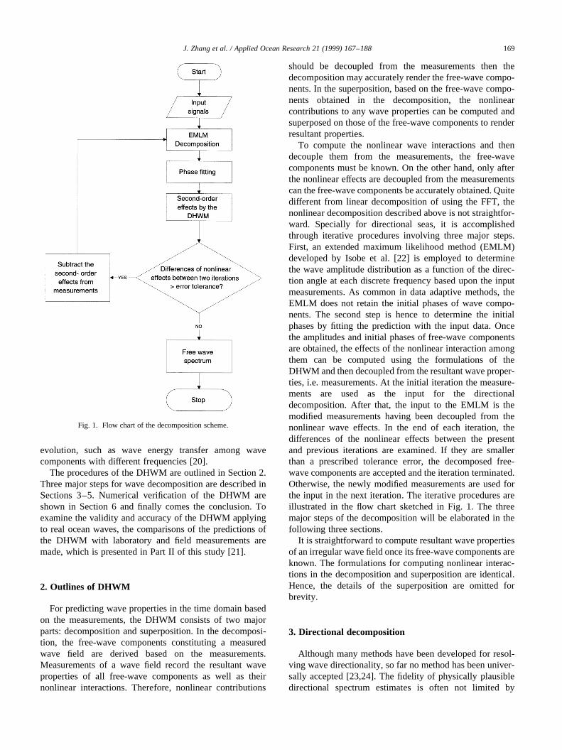
To compute the nonlinear wave interactions and thendecouple them from the measurements, the free-wavecomponents must be known. On the other hand, only afterthe nonlinear effects are decoupled from the measurementscan the free-wave components be accurately obtained. Quitedifferent from linear decomposition of using the FFT, thenonlinear decomposition described above is not straightfor-ward. Specially for directional seas, it is accomplishedthrough iterative procedures involving three major steps.First, an extended maximum likelihood method (EMLM)developed by Isobe et al. [22] is employed to determinethe wave amplitude distribution as a function of the direc-tion angle at each discrete frequency based upon the inputmeasurements. As common in data adaptive methods, theEMLM does not retain the initial phases of wave compo-nents. The second step is hence to determine the initialphases by fitting the prediction with the input data. Oncethe amplitudes and initial phases of free-wave componentsare obtained, the effects of the nonlinear interaction amongthem can be computed using the formulations of theDHWM and then decoupled from the resultant wave proper-ties, i.e. measurements. At the initial iteration the measure-ments are used as the input for the directionaldecomposition. After that, the input to the EMLM is themodified measurements having been decoupled from thenonlinear wave effects. In the end of each iteration, thedifferences of the nonlinear effects between the presentand previous iterations are examined. If they are smallerthan a prescribed tolerance error, the decomposed free-wave components are accepted and the iteration terminated.Otherwise, the newly modified measurements are used forthe input in the next iteration. The iterative procedures areillustrated in the flow chart sketched in Fig. 1. The threemajor steps of the decomposition will be elaborated in thefollowing three sections.

It is straightforward to compute resultant wave propertiesof an irregular wave field once its free-wave components areknown. The formulations for computing nonlinear interac-tions in the decomposition and superposition are identical.Hence, the details of the superposition are omitted forbrevity.

3. Directional decomposition

Although many methods have been developed for resol-ving wave directionality, so far no method has been univer-sally accepted [23,24]. The fidelity of physically plausibledirectional spectrum estimates is often not limited by

J. Zhang et al. / Applied Ocean Research 21 (1999) 167–188 169

Fig. 1. Flow chart of the decomposition scheme.

estimation techniques but by the resolving power ofmeasured array data, which depend on the number ofmeasuring instruments and their layout [25]. In practice,the resolution of the instrument array is often limited.Considering ocean waves being recorded at sparse points,data adaptive methods are used to estimate wave directionalspreading. Two methods, maximum likelihood method(MLM) and maximum entropy method (MEM), are mostwidely used because of their resolution power and theirflexibility. Both methods have been extended for the appli-cations to multiple array data of different wave properties,and are respectively named as extended maximum likeli-hood method (EMLM) [22] and extended maximum entropymethod (EMEM) [26]. Although EMEM can detect partiallyreflected waves more accurately by resorting to additionalphysical constraints, the EMLM is much less intensive incomputing than the EMEM and has the same resolutionpower as the former in most scenarios. Therefore, theEMLM is employed in the DHWM to estimate the direc-tional spreading of a measured wave field. The algorithm ofEMLM was given by Isobe et al. [22] and omitted here forbrevity. In this study, it is assumed that the measured wavefield is uni-modal. That is, at each frequency waves spreadaround one main direction but the main directions of waveat different frequencies may vary. In nature, bi-modal wavesmay be caused by wave reflection from the walls of wavebasins, structures and coastlines. To accurately estimatewave directionality of a bi-modal wave field, additionalinformation, such as the position of walls and coastlines,and special layout of measuring instruments are required.Under these circumstances, the EMLM can be replaced bythe EMEM for estimating wave spreading in the DHWMwithout principal difficulties.

The directional resolution of the EMLM is set to fourdegrees in this study, resulting in 90 directional componentsfor each discrete frequency. The number of discretefrequencies is of order of hundreds and determined by theduration of the time-series and the cutoff frequency. Fromthe view of computation, 90 directional free-wave compo-nents at each frequency are too many. Besides, the initialphases of 90 directional wave components cannot be accu-rately determined by a few point measurements. Therefore,only a limited number, 2N 1 1, of free-wave components ateach frequency are selected from the 90 components torepresent the directional spreading obtained using theEMLM. For narrow directional wave spreading, one direc-tional wave component at each discrete frequency might beadequate. While for broad directional wave spreading, 2N 11 � 3, 5 and 7 will be considered. Hence, the number ofdirectional wave components to be used at each frequencydepends on the directional spreading of the measured oceanwaves. The number and directions of selected componentsat each frequency are determined first and then their waveamplitudes are scaled to conserve the total energy at eachfrequency. It is elucidated below.

Given the directional spreading at each frequency, the

component with the largest amplitude, defined as the mostenergetic component, can be identified and its propagationdirection is taken as the main direction of wave propagationat this frequency. If only one component is employed ateach frequency, its direction is taken as the main propaga-tion direction. To conserve the energy, the amplitude of therepresentative component must be scaled, that is, multipliedby a scale factorm ,

m �

��XMi�1

A2i

A2max

vuuuut; �1�

whereAi andAmax are the amplitudes of theith directionalfree-wave component and the most energetic free-wavecomponent, respectively, at a discrete frequency, whichare obtained using the EMLM.M is the number of direc-tional wave components andM � 90 is used in ourcomputation. After scaling the amplitude of the representa-tive free-wave component at this frequency is equal tomAmax.

When the directional spreading is wide, more than onecomponent at each frequency should be used to achieve abetter approximation of wave spreading. The criteria ofdetermining the number 2N 1 1 is based on the squareroot of the normalized second directional angular moment.

P �

��XMi�1

�Ai�bi 2 b0��2

XMi�1

A2i

vuuuuuuuut ; �2�

whereb i andb0 are the directional angles ofith directionalfree-wave component and the most energetic free-wavecomponent, respectively. If the wave energy focuses atone direction (no spreading) at this frequency, the secondmoment is equal to zero. If the energy spreading isuniformly distribution in all directions, the second momentis p2/3. The value ofP defined in Eq. (2) indicates theextent of directional spreading of a measured wave field.When it is relatively small, 2N 1 1 is chosen to be unity.While P is large, say greater than 0.20, 2N 1 1 may bechosen from 3, 5 and 7.

For describing the procedures of determining 2N 1 1representatives at each frequency, the indices of the 90components at each frequency are shifted so that the indexof the most energetic wave component isM/2 1 1� 46 andeach one half of the amplitude of the wave component in theopposite direction of the most energetic component isplaced atj � 1 and j � 91, respectively. Hence, there areequally 45 wave components at left-hand side (j � 1 to 45)and right-hand side (j � 47 to 91) of the most energetic free-wave component. First, we determine the directions of the2N 1 1 representatives. The direction of the most energeticcomponent is chosen to be one of the 2N 1 1 representa-tives. In addition to that, there are equallyN representative


components at both sides of the most energetic component.In anticipation that the spreading at the two sides may beasymmetric with respect to the most energetic component,the directions of theN representative components at left-hand and right-hand sides are determined separately basedon the first and second moments of each side. Given belowis the procedure of selecting the directions ofN free-waverepresentatives at the left-hand side. The procedure for thoseat the right-hand side is similar.

The normalized first and second angular momentsM1 andM2 at left-hand side are defined as,

M1 �

X45

j�1

A2j �bj 2 b0�

X45

j�1

A2j

; �3�

M2 �

X45

j�1

A2j �bj 2 b0�2

X45

j�1

A2j

; �4�

whereAj andb j are the amplitude and directional angle ofthe jth component at the left-hand side of the most energeticcomponent, respectively. The ratio,M2/M1, is chosen as thedirection of the most left representative component. IfN .1, the directional angles of the remaining representativecomponents are evenly distributed between the angles ofthe most left and most energetic components. Because ofthe discrete directional angles used in the computation, thedirections of representative components are rounded to themultiple of four degrees.

Once the directions of all representative components havebeen determined, their amplitudes are scaled by multiplyinga factorm , to conserve the energy at this frequency. Thescale factor is

m �

��X91

i�1

A2i

X2N 1 1

m�1

B2m

vuuuuuuuut ; �5�

whereBm is a subset ofAi, and is defined byBm� Ai. Bm (form� 1 to 2N 1 1) have the same directions of the represen-tative components.

4. Determining initial phases

After the amplitudes and directions of the representativefree-wave components at each frequency are calculated,their initial phases need to be determined based on themeasurements, which is described below.

The initial phases of the free-wave components at each

frequency are determined by minimizing a target functiondefined as,

Rn �XJj�1

uDjn

Hju2; �6a�

Djn �X2N 1 1

m�1

Hjanmei�knm·xj11nm� 1 1jn 2 Ejneifjn ; �6b�

whereDjn is the difference between a predicted wave prop-erty and the corresponding measurements of thejth sensor atthenth frequency. This predicted property is the same typeas the measurement and at the same location. The uppersummation indexJ stands for the total number of inputmeasurements in the decomposition and 2N 1 1 the totalnumber of the free-wave components atnth frequency asdescribed in the previous section. The predicted property isthe superposition of linear and nonlinear contributionswhich are described by the first and second terms at theright hand side of Eq. (6b), respectively.anm, knm, andenm

denote the elevation amplitude, wavenumber vector andinitial phase of themth free-wave component atnthfrequency, respectively.xj is the horizontal coordinatesvector of thejth sensor.Hj is the linear transfer functionof the elevation amplitude to the measured wave propertyat the jth sensor. If the measured property is the surfaceelevation, thenHj � 1. The nonlinear contribution at thenth frequency and the location of thejth sensor,e jn, canbe calculated using the formulations described in the nextsection. The last term at the right-hand side of (6b) is theFFT coefficient of the measurement at thejth sensor, andEjn

and f jn stand for the modulus and phase at thenthfrequency, respectively.

Since the total number of input measurements isJ and thetotal number of free-wave components is 2N 1 1 at eachfrequency, we have 2J real equations to solve for 2N 1 1unknown initial phases. The minimum number of inputmeasurements is three. In general, 2N 1 1 is not requiredto equal, but usually smaller than 2J. Therefore, it is anover-determined problem if 2J . 2N 1 1. Consequently,the initial phases are obtained by minimizing the targetfunction defined in Eq. (6a). The minimization is performedby systematically varying the magnitudes of the initialphases in a multi-dimensional space of dimension 2N 1 1.It can be accelerated using a conjugate gradient minimiza-tion algorithm, known as the Fletcher–Reeves–Polak–Ribiere method [27]. The computation is completed whenthe target function is smaller than a preset error tolerance.

5. Computation of nonlinear contributions

5.1. Governing equations

For an incompressible and irrotational flow with a freesurface, the governing equation and boundary conditions


can be written as

72F � 0; 2h # z # z; �7�

2F

2t1

12

u7Fu2 1 gz � C0 at z� z; �8�

2z

2t1

2F

2x2z

2x1

2F

2y2z

2y� 2F

2zat z� z; �9�

2F

2z� 0 atz� 2h; �10�

whereF is the velocity potential (the velocity potential isrelated to the velocity vector through7F � V), z thesurface elevation,t time, g the gravitational accelerationand h the water depth which is assumed to be uniform.The x and y axes are in the horizontal plane, and thez-axis is pointing upwards.C0 is the Bernoulli constantwhich will be chosen to ensurez � 0 located at the stillwater level.

Longuet-Higgins and Stewart [28] used the conventionalperturbation method to derive the solutions for wave–waveinteraction in the order of wave steepness, defined as theproduct of the wavenumber and amplitude. When the wave-length ratio of the short to long wave,e l, is of O(1), theconventional perturbation solution converges veryquickly. However, whene l is small and approaches thelong-wave steepnesse1, the truncated solution may diverge[16].

The phase modulation method [16,29] provides a comple-mentary solution to the conventional perturbation method. Itconsiders the consequence of wave interactions as themodulation of a short-wave component by a long-wavecomponent and describes it directly in the solution of theshort-wave component. In the case of long-crested waves,the phase modulation solution has been proved to be iden-tical to the conventional solution up to third-order in wavesteepness whene1 p e l , 0.5. However, ase1 becomeslarger and greater thane l, the conventional solutiondiverges, while the phase modulation solution remainsconvergent. But, whene l . 0.5, the phase modulationmethod cannot accurately predict the slowly varying inter-action between the two wave components at third order[16,30].

5.1.1. Conventional solutionsThe conventional solution for the potential of two inter-

acting directional wave components in an intermediate-depth water was given by Longuet-Higgins [31] and Hsu

et al. [32],

F �X2i�1

(aigsi

cosh�ki�z1 h��cosh�kih� sinui

138

a2i sicosh�2ki�z1 h��

sinh4�kih�sin�2ui�

)

1a1a2s2

2A�2�

cosh�uk1 2 k2u�z1 h��cosh�uk1 2 k2uh� sin�u1 2 u2�

1a1a2s2

2A�1�

cosh�uk1 1 k2u�z1 h��cosh�uk1 1 k2uh� sin�u1 1 u2�;

�11�where

A�7�

� 7k2�2l�1 7 l��Ga1a2 ^ 1�7 l3�a2

1 2 1�1 a22 2 1�

k2�1 7 l�2 2 a2uk1 7 k2utanh�uk1 7 k2uh� ;

�12a�

l � s1

s2; �12b�

ai � coth�kih�; i � 1; 2; �12c�

G � cos�b1 2 b2�; �12d�

ui � kixx 1 kiyy 2 si t 1 di ; i � 1; 2; �12e�with ai, b i, ki, s i andd i representing the wave amplitude,directional angle with respect to thex-axis, wavenumbervector, frequency and initial phase of theith wave compo-nent,ki is the modulus of the wavenumber vector,ki � uk iu,kix andkiy represents thex- andy-components ofk i, respec-tively. By default, a smaller subscript indicates a lowerfrequency of the wave component, i.e.s1 , s2. Thesubscripts of (1 ) and (2 ) indicate the sum- and differ-ent-frequency interactions, respectively. The solution forthe surface elevation is given by,

z �X2i�1

(aicosui 1

a2i s

2i

4g

"2 1

3cosh�2kih�sinh4�kih�

21

sinh2�kih�

#cos 2ui

)1

a1a2k2

2a2�2�1 2 l�A�2�

1 M�2��cos�u1 2 u2�1a1a2k2

2a2��1 1 l�A�1�

1 M�1��cos�u1 1 u2�; �13a�where

M�7� � l2 1 1 2 l�Ga1a2 ^ 1�: �13b�


The Bernoulli constant is found to be

C0 �X2i�1

a2i ki

21

sinh 2kih: �14�

5.1.2. Phase modulation solutionThe phase modulation method was extended to study two

interacting directional waves in deep water by Hong [33].His results revealed the structure of the solutions for themodulated wave phase, amplitude and potential of a short-wave component. However, Hong’s derivation is lengthyand complicated because of the conformal mappingbetween two different solution domains. To simplify thederivation, a new modulation perturbation scheme is devel-oped here to derive the solution directly in the Cartesiancoordinates. Furthermore, our solutions allow for an inter-mediate-water depth with respect to the long-wave compo-nent.

In contrast to the conventional method, the phase modu-lation method considers the consequence of wave interac-tions as the modulation on the short-wave component. For adirectional deep-water short-wave component modulated byan intermediate water-depth long-wave component, weexplicitly formulate the modulation in the solutions for thefirst harmonic short-wave potential and elevation accordingto the features discovered by Hong [33] and then determinethe solutions using the governing Eq. (18) and boundaryconditions (19)–(21).

The total potential and surface elevation can be expressedas a superposition of the potentials and elevations of a short-wave and a long-wave components,

F � F1 1 F3; �15�

z � z1 1 z3; �16�where the subscripts 1 and 3 stand for the long-wave andshort-wave components, respectively. The governing equa-tion and boundary conditions forF are the same as (7)–(10)except that the bottom boundary condition for the short-wave component is changed to a deep-water constraint,

7F3 ! 0 asz! 2h: �17�The effect of the interaction on the long-wave component

is known to be at most of third-order in wave steepness[30,33]. Hence, the solution for the long-wave componentup to the second order is the same as that of a single Stokeswave train. By expanding the free surface boundary condi-tions at the undisturbed long-wave surface and subtractingthe surface boundary conditions for the long-wave compo-nent alone, we obtain the governing equation and boundaryconditions for the short-wave component, accurate up to thesecond order in wave steepnesses,

72F3 � 0; 2h # z # z1; �18�

2F3

2t1 gz3 1 7F1·7F3 1

22F1

2t2zz3 1

12

u7F3u2 122F3

2t2zz3

� 0

at z� z1; �19�

2z3

2t2

2F3

2z1 7hF1·7hz3 1 7hF3·7hz1 2

22F1

2z2 z3

17hF3·7hz3 222F3

2z2 z3 � 0 atz� z1; �20�

7F3 ! 0 asz! 2h; �21�wherefh is the horizontal gradient operator. The last twoterms at the left-hand-sides of Eqs. (19) and (20) are ofsecond order and result from the interaction of the short-wave component with itself. Thus, they only contribute tothe second harmonic of the short-wave component andconsequently can be ignored in the derivation of the modu-lations of the first harmonic of the short-wave component.The remaining nonlinear terms in Eqs. (19) and (20) repre-sent the interaction between the long-wave and short-wavecomponents. Because the second harmonic of the short-wave component is of the second-order, the modulationon the second harmonic are of third-order. The solutionfor the second harmonic of short-wave component up tothe second-order is hence the same as a single Stokeswave and its derivation is omitted for brevity.

Based on the modulation features revealed by Hong’sresults [33], the modulated short-wave component potentialand elevation can be formulated as,

F3 � A3fAek3fksin ~u 3; �22�

z3 � a3�1 1 11bcosu1�cos ~u 3; �23�where

fA � 1 1 11tcosu1; �24a�

fk � z2 a1cosu1 1 11zcosu1

XJj�0

gj�k1z�j ; �24b�

~u 3 � k3xx 1 k3yy 2 s3t 1 d3 1 k3a1 sinu1

XJ 1 1

j�0

rj�k1z�j ;

�24c�~u 3 � k3xx 1 k3yy 2 s3t 1 d3 1 k3a1r0 sinu1 1 D11 sinu1;

�24d�andA3, fA are respectively the average potential amplitudeand its corresponding modulation factor. Herefk denotes theeffects of the changes in the short wavenumber and therelative still water level with respect to the short-wave


components owing to the presence of the long-wave compo-nent. ~u 3 and ~~u3 are the modulated phases for the potentialand surface elevation, respectively. They are modeled as thesum of the linear phase and the modulation by the long-wave component.b stands for the modulation of theelevation amplitude andD is the phase shift between theelevation phase and the potential phase at the free surface.The parameters,r , g , t andb, can be further expanded interms of the frequency ratio of the long-wave to the short-wave component,l ,

rj �X2�J 1 1�2 2j

n�0

lnrjn; gj �X2J 2 2j

n�0

lngjn;

t �X2J

n�0

lntn; b�X2J

n�0

lnbn;

�25�

where the summation is set to be zero if its upper limit isnegative. All unknown coefficients related to the modulationwill be determined using the Laplace equation and boundaryconditions.

From the view of mathematical formulations, the modu-lated potential is a more general solution to the Laplaceequation than the conventional one. The conventionalpotential is formulated for the use of the variable separationmethod for solving the Laplace equation. It is the product oftwo functions with one of them depending solely on thevertical coordinate and the other on the horizontal coordi-nates. In the modulated potential as shown in Eq. (22), thetwo corresponding functions not only depend strongly onthe same variables as in the conventional potential, but alsodepend weakly on additional variables. For example, theexponential function strongly depends onzand also weaklydepends onx, y and t. If this weak dependence on othervariables can be separated at relatively lower orders themodulated potential reduces to the conventional potential.If the separation of this weak dependence cannot be trun-cated at lower orders, the solutions for the two potentialsmay be qualitatively different. That is why the phase modu-lation method can provide convergent solution and theconventional method cannot in the cases such as short-and long-wave interactions. On the other hand, because ofthe formulation of the modulated potential, the Laplaceequation can no longer be easily solved using the variableseparation. This is the price to pay for using the phasemodulation method to obtain a convergent solution trun-cated at lower orders.

Since the phase modulation method is applied to the inter-actions between wave components with quite differentwavelengths,l is expected to be relatively small. Generallyspeaking, it is smaller than 0.5. Theoretically, the series inEqs. (24b), (24c) and (25) can be extended to infinity, but innumerical computation they have to be truncated. It will beshown that the magnitude ofk1z is of O(l 2). Hence, theseries in the double summations of Eqs. (24b) and (24c)converge quickly ifl p 1. To achieve an accuracy at

certain order ofl for the solutions of the potential andelevation, the truncations of the summations in Eqs. (24b),(24c) and (25), have to be made consistently. For example,the truncation ofr j in Eq. (25) depends on the subscriptsjand the upper limit integerJ in the summations of Eqs. (24b)and (24c). The reasons are elaborated below.

For nontrivial magnitude of the short-wave potential, theabsolute value of its exponential indexk3zshould be of O(1).Because ofk1=k3 � a1l

2; we haveuk1zu , O�a1l

2�: Further-more, because the water depth is intermediate with respectto the long-wave component,a1 , O�1�: Hence, uk1zu ,O�l2� and �k1z�j , O�l2j�: If r j is truncated at 2(J 1 1) 22j, thenr j11 should be truncated at 2(J 1 1) 2 2(j 1 1). Asa result,rj�k1z�j andrj11�k1z�j11 are accurate up to the sameorder, O(l 2(J11)). The truncation ing j can be made simi-larly. Becauset andb only involve a single summation, toachieve the same accuracy their summations in Eq. (25) aretruncated at 2J. As a result, the truncated solutions for theshort-wave potential and elevation are accurate up toO�11l

2J�:Substitution of Eq. (22) into the Laplace equation (18)

gives,

Eek3fksin ~u 3cosu1 11k23 1 Fek3fk cos ~u 3 sinu111k2

3 � 0; �26�whereE andF are given by

E � 2l4a21t 2 2G

XJj�0

rj�k1z�j 1 l2a1 1 2XJj�0

gj�k1z�j11

24 351 2

XJj�0

�j 1 1�gj�k1z�j 1 l2a1

XJ 2 1

j�0

�j 1 1� �27a�

� �j 1 2�gj11�k1z�j ;

F � 22l2a1Gt 1 2G 1 2XJj�0

gj�k1z�j11

24 352 l2a1

XJj�0

rj�k1z�j

1 2XJj�1

jrj�k1z�j21 1 l2a1

XJ 2 1

j�1

j�j 1 1�rj11�k1z�j21;

�27b�

with G being as defined in Eq. (12d). Splitting Eq. (26) withrespect to sin~u 3 and cos~u 3; we have two equations,E� 0andF� 0, that may be satisfied by letting each coefficient ofthe terms, (k1z)

m, be zero. From the equationE � 0, thefollowing equations are obtained,

O�1� : 22Gr0 2 l4a21t 1 l2a1 1 2g0 1 2l2a1g1 � 0;

�28a�


O�km1 zm� : 22Grm 2 l2a1gm21 1 2�m1 1�gm

1l2a1�m1 1��m1 2�gm11 � 0;

m� 1;2;…

�28b�

Similarly, from F � 0,

O�1� : 2G 2 2l2a1tG 2 l2a1r0 1 2r1 1 2l2a1r2 � 0;

�29a�O�km

1 zm� : 22Ggm21 2 l2a1rm 1 2�m1 1�rm11

1l2a1�m1 1��m1 2�rm12 � 0; �29b�m� 1;2;…:

Eqs. (28) and (29) can be further expanded in the order ofl n. From Eq. (28a), we obtain the following hierarchyequations

O�1� : 22Gr00 1 2g00 � 0; �30a�

O�l� : 22Gr01 1 2g01 � 0; �30b�

O�l2� : 22Gr02 1 a1 1 2g02 1 2a1g10 � 0; �30c�

O�l3� : 22Gr03 1 2g03 1 2a1g11 � 0; �30d�

O�ln� : 22Gr0;n 1 2g0;n 2 a21tn24 1 2a1g1;n22 � 0;

n $ 4: (30e)

Similarly, Eq. (28b) can be expanded as, form� 1, 2,…,

O�1� : 22Grm;0 1 2�m1 1�gm;0 � 0; �31a�

O�l� : 22Grm;1 1 2�m1 1�gm;1 � 0; �31b�

O�ln� : 22Grm;n 2 a1gm21;n22 1 2�m1 1�gm;n

1�m1 1��m1 2�a1gm11;n22 � 0; �31c�n $ 2:

In the same way, Eq. (29a) is further expanded as

O�1� : 2r10 1 2G � 0; �32a�

O�l� : 2r11 � 0; �32b�

O�ln� : 2r1n 2 2a1tn22G 2 a1r0;n22 1 2a1r2;n22 � 0;

n $ 2: �32c�

and so is (29b) form� 1, 2,…,

O�1� : 22Ggm21;0 1 2�m1 1�rm11;0 � 0; �33a�

O�l� : 22Ggm21;1 1 2�m1 1�rm11;1 � 0; �33b�

O�ln� : 22Ggm21;n 2 a1rm;n22 1 2�m1 1�rm11;n

1�m1 1��m1 2�a1rm12;n22 � 0; �33c�n $ 2:

Eqs. (30)–(33) are used to express all coefficients ofr j andg j in terms ofr0�r00; r01;…; r0n�; andt�t0; t1; t2;…tn�; thatis detailed in Appendix A. The coefficientsr0, t , b andDcan be calculated using the free-surface boundary conditions.

Substitutingz3 andF3 into the boundary conditions (19)and (20) and perturbing them in the order of wave steepness,e1, we obtain the following hierarchy equations. For deriv-ing the solution up to second order,

O�1� : A3s3 � a3g; �34a�

O�11� :

2A3s3t 2 A3k3k211 s1�r0 2 a1G�1 a3g�b 2 a21

1 � � 0;

�34b�

A3s1t 2 a3gD � 0: �34c�

O�1� : a3s3 � A3k3; �35a�

O�11� :2A3k3�t 1 g0�1 a3�s3b 1 s1D�1 a3k3k21

1 s1�r0 2 a1G�� 0;

�35b�

2A3k3�G 1 r1�1 a3s3D 1 a3s1�b 2 a1� � 0: �35c�It should be noted that the equations atO(e1) have been

split with respect to the factors of sinu1 and cosu1. Eq.(34a) renders the relationship between the average potentialand elevation amplitudes,

A3 � a3gs3

: �36�

Combining Eqs. (34a) and (35a), the linear dispersion rela-tionship is obtained:s2

3 � gk3: Eq. (34c) relates the phaseshift D to t ,

D � lt: �37�Substituting Eqs. (36) and (37) into Eqs. (34b), (35b) and(35c) and noticingk1=k3 � l2a1; Eqs. (34b), (35b) and (35c)are reduced to,

2t 2 l21a211 r0 1 l21G 1 b 2 a21

1 � 0; �38a�

2t 2 g0 1 b 1 a211 l21r0 1 l2t 2 l21G � 0; �38b�

2G 2 r1 1 lt 1 lb 2 la1 � 0: �38c�Subtracting Eq. (38a) from Eq. (38b) and then subtractingEq. (38c) divided byl , from Eq. (38b), we eliminateb from


the system of equations:

2g0 1 a211 1 2a21

1 l21r0 1 l2t 2 2l21G � 0; �39a�22t 2 g0 1 a21

1 l21r0 1 l21r1 1 a1 1 l2t � 0: �39b�Sinceg0 andr1 can be calculated in terms ofr0 andt usingthe recursive relations resulting from the Laplace equationas described in Appendix A, there are only two unknownstandr0 in Eq. (39) and hence they can be solved. Eqs. (39a)and (39b) can be further perturbed in the order ofl . FromEq. (39a), we have the following set of equations,

O�l21� : r00 � Ga1; �40a�

O�l0� : r01 � 12�a1g00 2 1�; �40b�

O�l� : r02 � 12a1g01; �40c�

O�ln� : r0�n11� � a1

2�g0n 2 tn22�; n $ 2: �40d�

Similarly, Eq. (39b) can be perturbed into the following setof equations,

O�l21� : r10 � 2G; �41a�

O�l0� : t0 � 12�a21

1 r01 1 r11 2 g00 1 a1�; �41b�

O�l� : t1 � 12�a21

1 r02 1 r12 2 g01�; �41c�

O�ln� : tn � 12�a21

1 r0n11 1 r1n11 2 g0n 1 t0n22�;

n $ 2: (41d)

Noticingg00 � Gr00 � G2a1 from Eqs. (30a) and (40a),r01

can be calculated from Eq. (40b). Becauser00 andr01 areknown, the coefficientsgij �j � 0; 1� andrij �j � 0;1; i $ 2�can be obtained using the recursive relations (A2) and (A3)shown in Appendix A. Thenr02 andt0 can be calculated asshown in (40c) and (41b). Based on the recursive relation(32c), we obtain

r12 � a1�Gg0 112r00 2 r20�: �42�

Then t 1 can be calculated from (41c). The solutions forr0n11 and tn (when n $ 2) can be alternatively obtainedfrom lower to highern using (40d) and (41d). In the compu-tation,g0n andr1 n11 are computed using the recursive rela-tions described in Appendix A. The solutions forrij �i $ 2; j $ 2� and gij �j $ 1� can also be calculatedusing the recursive relations. Afterr0n andtn�n� 0;1;…�are obtained,bn�n� 0;1;…� can be calculated using(38a).

The solutions forr , g , t , andb are presented in AppendixB. Knowing these parameters, the potential and elevation ofthe modulated first-harmonic short-wave components canbe readily obtained from Eqs. (22)–(24).

5.1.3. Hybrid solutions for multiple interacting wavesA short-crested ocean wave field consists of many free-

wave components ranging from very low to relatively highfrequencies. For applying conventional and phase modula-tion solutions to wave–wave interactions in an ocean wave


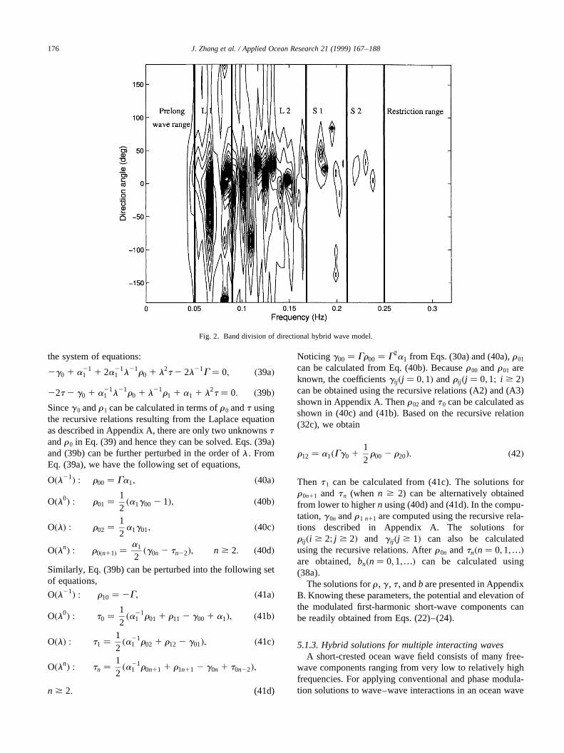
Fig. 2. Band division of directional hybrid wave model.

field, its spectrum is usually divided into three regions:pre-long, powerful and restriction regions as sketched inFig. 2. The powerful region involves all free-wavecomponents with relatively significant wave energyand is further divided into four bands, i.e. long-waveband one (L1) and two (L2) and short-wave band 1(S1) and 2 (S2), starting from low to high in thefrequency domain. For most ocean wave fields, thespectra peak is located in band L1. The amplitudesand especially the wave steepnesses of the free-wavecomponents in the pre-long wave region are verysmall. Hence, the interactions of a free-wave com-ponent in the pre-long wave region with any free-wave components are insignificant and neglected. It isalso assumed that the wave components in the restric-tion region are mainly the bound-wave componentsresulting from the interactions among the free-wavecomponents in the wave bands of L1, L2, S1 and S2.Therefore, the cut-off frequency for the free-wavecomponents is that at the end of S2.

Two free-wave components located in the samefrequency band or in neighboring bands are relativelyclose in frequency and hence the interaction between themis calculated using the conventional solution. Two free-wave components located in two different bands separatedby at least one other band are relatively far apart infrequency and hence are calculated using the phase modula-tion solution. For simplicity of illustration, the solutions forwave–wave interactions in an irregular wave field of multi-ple free-wave components are described for the case of itspowerful range involving three wave bands: two long-wavebands (L1 and L2) and one short-wave band (S1). Theextension of the above solution for more than three wavebands is straightforward.

The interactions between the free-wave components inL1 and L2 are calculated using the conventional perturba-tion method, likewise, for the interactions between the free-wave components in L2 and S1. However, the interactionsbetween the two free-wave components located respectivelyin L1 and S1 are computed using the phase modulationmethod. The total potential of a directional wave fieldconsists of the following parts,

F � FL1 1 FL2 1 FS1L1 1 FS1L2 1 FSS; �43�

whereFL1 andFL2 are the resultant potentials of L1 and L2,including the potentials of all free-wave components inthese two bands and the nonlinear interactions betweenthem. HereFS1L1 is the total first harmonic potentials ofcomponents in S1 modulated by L1,FS1L2 is the total poten-tial resulting from the nonlinear interactions between L2and S1 andFSSthe total potential from interactions betweenthe free-wave components in S1. In the following formula-tions, it is assumed that there areM1 and M2 frequencyincrements in L1 and L2, andN frequency increments inS1, and there is only one free-wave component at each

frequency. These potentials can be calculated by:

FL1 1 FL2

�XMj�1

(ajg

sj

cosh�kj�z1 h��cosh�kjh� sinuj

138

a2j sjcosh�2kj�z1 h��

sinh4�kjh�sin�2uj�

)�44�

1XMj�2

Xj 2 1

i�1

(aiajsj

2Aj2i

cosh�ukj 2 ki u�z1 h��cosh�ukj 2 ki uh�

sin�uj 2 ui�

1aiajsj

2Aj1i


sin�uj 1 ui�);

whereM � M1 1 M2, Aj2i andAj1i are the same asA(2) andA(1) given in (12a) except that the subscripts 1 and 2 arereplaced byi and j, respectively.

FS1L1�XM 1 N

j�M 1 1

Fj ; �45�

whereF j is determined in the same way asF3 in (22) exceptthat the modulation factorsfA and fk, and the modulatedphase ~u j need to be extended to allow for the modulationby multiple long-wave components in L1,

fAj � 1 1XM1

i�1

1itij cosui ; �46�

fkj � z2XM1

i�1

aicosui 1 1izcosui

XJl�0

glij �kiz�l" #( )

; �47�

~u j � kjxx 1 kjyy 2 sj t 1 dj 1XM1

i�1

kjai sinui

XJ 1 1

l�0

rlij �klz�l" #

;

�48�where the subscripts ofi and j stand for ith long-wavecomponent andjth short-wave component, respectively.

FSS 1 FS1L2

�XM 1 N

j�M 1 1

38

a2j sjcosh�2kj�z1 h��

sinh4�kjh�sin�2uj�1

XM 1 N

j�M 1 2

Xj 2 1

i�M 1 1

1XM 1 N

j�M 1 1

XMi�M1 1 1

!�49�

�(

aiajsj

2Aj2i


sin�uj 2 ui�

1aiajsj

2Ai1j


sin�uj 1 ui�):


Similarly, we can express the surface elevationz as

z � zL1 1 zL2 1 zS1L1 1 zS1L2 1 zSS; �50�where the right-hand-side terms represent the parts of thesurface elevation corresponding to the potentials with thesame subscripts in (43).

zL1 1 zL2

�XMj�1

ajcosuj 1XMj�1

a2j s

2j

4g

"2 1

3cosh�2kjh�sinh4�kjh�

21

sinh2�kjh�

#cos 2uj �51�

1XMj�2

Xj 2 1

i�1

(aiajkj

2aj�2�1 2 l�Aj2i 1 Mj2i�

× cos�uj 2 ui�aiajkj

2aj��1 1 l�Ai1j 1 Mi1j�cos�ui 1 uj�

):

zS1L1�XM 1 N

j�M 1 1

aj 1 1XM1

i�1

1ibji cosui

!cos ~~u j ; �52�

wherebji is the valueb for jth short-wave component modu-lated byith long-wave component and

~~u j � kjxx 1 kjyy 2 sj t 1 dj 1XMi�1

kjair0ij sinui

1XMi�1

1iDij sinui ;

�53�

in which r0ji andD ij are the coefficientsr0 andD of jthshort-wave component modulated byith long-wave compo-nent, respectively. We also obtain

zSS 1 zS1L2

�XNj�1

a2j kj

2cos2uj 1

XM 1 N

j�M 1 2

Xj 2 1

i�M 1 1

1XM 1 N

j�M 1 1

XMi�M1 1 1

!

×(

aiajkj

2aj�2�1 2 l�Aj2i 1 Mj2i�cos�uj 2 ui� �54�

1aiajkj

2aj��1 1 l�Ai1j 1 Mi1j�cos�ui 1 uj�

):

The solutions for pressure, velocity and acceleration canbe derived based on the potential and are omitted forbrevity.

5.1.4. Criteria for region and band divisionAccording to our definition, all wave components in the

pre-long wave and restrictive regions must be of smallamplitude. The upper limit index for the pre-long waveregion is hence determined by the criterion that the ampli-tude of any wave components in this region is below apercentage (5 to 10%) of the amplitude at the frequencyspectrum peak. The cutoff frequency is set such that theamplitudes of any wave components of frequencies abovethe cutoff frequency are smaller than 1–2% of the amplitudeat the spectrum peak. The lower limit index for the powerfulregion is the next to the upper limit index of the pre-longwave region. The division of bands in the powerful region isconducted according to two criteria.

First, the width of each band must be narrow enough sothat the corresponding truncated conventional solutions canbe applied to calculate the interactions between free-wavecomponents located in the neighboring bands. Hence, thewidth of each band is limited by the maximum of an equiva-lent wave steepness in the time series used in the wavedecomposition.

max u1eu p 1; �55�where the equivalent wave steepness,ee, is defined by,

1e � kN

XMu

j�Ml

cos�bj 2 bN�ajaj sinuj ; �56�

and Ml and Mu respectively denotes the lower and upperlimit indices of a band, and the subscriptN is the index ofthe free-wave component of the highest frequency in thenext band. By comparing Eqs. (56) and (53), we may findthat ee is essentially the leading-order phase modulation ofthe free-wave component of indexN in the next band, whichresults from the modulation by all free-wave component ofindices betweenMl andMu. If the criterion is satisfied, theinteractions between free-wave components in the neigh-boring bands can be calculated using the conventional solu-tion. Otherwise, we may either choose a smallerMu toreduce the bandwidth (Mu 2 Ml 1 1), or choose a smallerN to reduce the bandwidth of next band (N 2 Mu), or slightlyreduce the band widths of both bands.

The second criterion considers the assumption made inthe phase modulation method that the water depth is deepwith respect to the short-wave band components. The divi-sion between the long-wave band L2 and short-wave bandS1 is hence examined whether or not this assumption isvalid. It is not appropriate to apply the present wavemodel to irregular waves in relatively shallow water. Thislimitation can be removed if the current formulation of thephase modulation approach is extended to allow for an inter-mediate water depth with respect to the short-wavecomponent.

5.2. Decoupling nonlinear effects from measurements

Since the modulation of a short wave by a long wave issignificant and the influence of the short wave on the long


wave is at least one order higher [33], the decoupling of thenonlinear effects from the resultant wave properties isperformed in the order from the longest wave band to theshortest wave band. In conjunction with the hybrid solutionsdescribed in the previous section, the potential and elevationof wave components in the long- and short-wave bands areformulated differently. Consequently, the decoupling proce-dures are different in these wave bands.

An input measurement can be deterministically describedby cos and sin spectraac

j andasj based on the FFT.

ajcos�k j·x 2 st 1 bj� � acj cos�st�1 as

j sin�st�; �57�where

acj � ajcos�k j·x 1 bj�; �58a�

asj � ajsin�k j·x 1 bj�; �58b�

andx denotes the horizontal location of the measurement.We remark thatac

j and asj can have negative values. The

decoupling of nonlinear contributions from the measure-ments are mainly performed in the cos and sin spectra,which is equivalent to the computation made in the timedomain.

The conventional method renders the solutions for thenonlinear interactions in the frequency domain. The decou-pling from the measurements can be accomplished by thesubtraction of them from the cos and sin spectra. The phasemodulation method calculates the modulation of short-wavecomponents in the time domain. There are two approachesto decouple the nonlinear effects due to the modulation ofshort free-wave components. For the cases of one free-wavecomponent used at each discrete frequency, the decoupleprocess is virtually identical to that described in Zhang etal. [2]. The modulation of short-wave components of unitamplitude by the long-wave components is calculated in thetime domain and then transferred to the frequency domainusing the FFT and stored in a transfer matrix [C]. Theunmodulated free-wave components in a short-wave bandare then obtained by solving a set of simultaneous equations,[C]{ Af} � { AR}. The column vector, {AR}, is the modifiedmeasurement in the frequency bandwidth of the short-waveband. The word ‘modified’ indicates that other nonlineareffects, such as interactions between long-wave compo-nents, have been decoupled from the measurements.Detailed description about the algorithm of computing thecoefficient matrix [C] can be found in Zhang et al. [2]. Afterthe free-wave components in the short-wave band, {Af}, arecalculated, the modulation effects in the frequency domainoutside the frequency range of the corresponding short-wave band are computed and then subtracted from the modi-fied wave spectra. Furthermore, the second harmonics andthe interaction between the free-wave components withinthis short-wave band and neighboring long-wave band arecalculated and decoupled from the modified wave spectra.However, when multiple free-wave components are used ateach frequency, the above decoupling method cannot be

applied. An alternative method of decoupling the modula-tion of short-wave components is to subtract it from themodified spectra. The differences between the elevations(or other measured wave properties) of modulated short-wave components and the corresponding unmodulatedcomponents are viewed as the nonlinear effects due to themodulation by long-wave components. They can be calcu-lated for given free long-wave and short-wave components.It is observed that the two approaches render almostidentical results in the cases of one free-wave componentat each frequency.

6. Numerical verifications

Before the DHWM is applied to laboratory and fieldmeasurements, three types of numerical tests are conductedto ensure that its numerical scheme is reliable and conver-gent. The first type of tests is to explore the consistency anddifference between the conventional and phase modulationsolutions. The second type is to examine the consistencybetween the DHWM and already established unidirectionalhybrid wave model (UHWM) in the cases of unidirectionalirregular waves. The third type is to confirm that the decom-position renders convergent and unique free-wave compo-nents in decomposing a synthetic wave field consisting ofgiven free-wave components.

6.1. Comparison of conventional and phase modulationresults

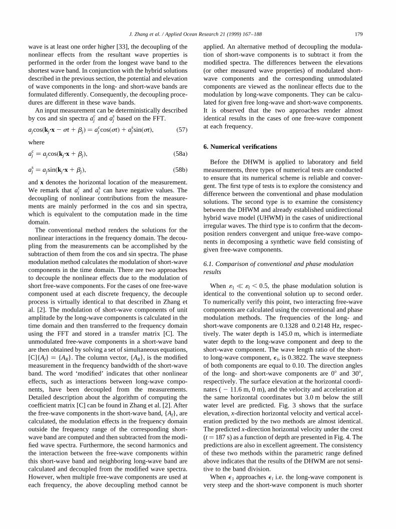
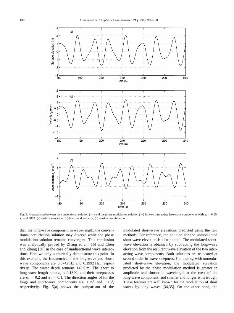
When 11 p 1l , 0:5; the phase modulation solution isidentical to the conventional solution up to second order.To numerically verify this point, two interacting free-wavecomponents are calculated using the conventional and phasemodulation methods. The frequencies of the long- andshort-wave components are 0.1328 and 0.2148 Hz, respec-tively. The water depth is 145.0 m, which is intermediatewater depth to the long-wave component and deep to theshort-wave component. The wave length ratio of the short-to long-wave component,e l, is 0.3822. The wave steepnessof both components are equal to 0.10. The direction anglesof the long- and short-wave components are 08 and 308,respectively. The surface elevation at the horizontal coordi-nates (2 11.6 m, 0 m), and the velocity and acceleration atthe same horizontal coordinates but 3.0 m below the stillwater level are predicted. Fig. 3 shows that the surfaceelevation,x-direction horizontal velocity and vertical accel-eration predicted by the two methods are almost identical.The predictedx-direction horizontal velocity under the crest(t� 187 s) as a function of depth are presented in Fig. 4. Thepredictions are also in excellent agreement. The consistencyof these two methods within the parametric range definedabove indicates that the results of the DHWM are not sensi-tive to the band division.

Whene1 approachese l i.e. the long-wave component isvery steep and the short-wave component is much shorter


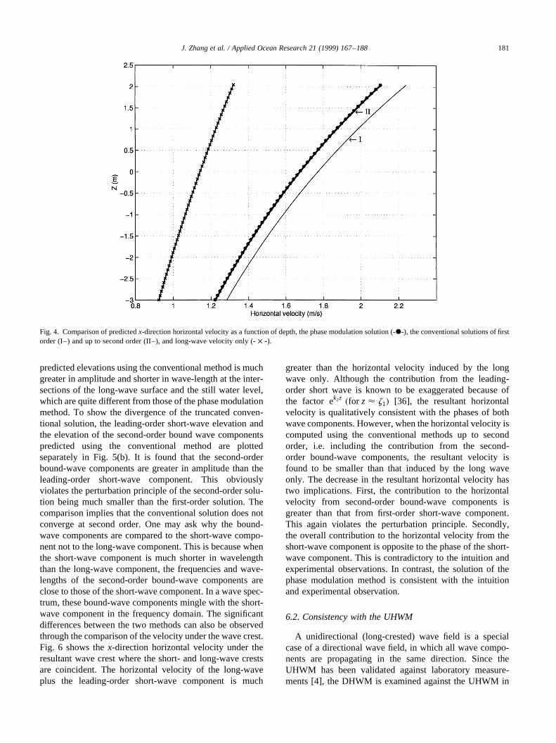
than the long-wave component in wave-length, the conven-tional perturbation solution may diverge while the phasemodulation solution remains convergent. This conclusionwas analytically proved by Zhang et al. [16] and Chenand Zhang [30] in the case of unidirectional wave interac-tions. Here we only numerically demonstrate this point. Inthis example, the frequencies of the long-wave and short-wave components are 0.0742 Hz and 0.1992 Hz, respec-tively. The water depth remains 145.0 m. The short tolong wave length ratioe l is 0.1390, and their steepnessesaree1 � 0.2 ande3 � 0.1. The direction angles of for thelong- and short-wave components are1158 and 2158,respectively. Fig. 5(a) shows the comparison of the

modulated short-wave elevations predicted using the twomethods. For reference, the solution for the unmodulatedshort-wave elevation is also plotted. The modulated short-wave elevation is obtained by subtracting the long-waveelevation from the resultant wave elevation of the two inter-acting wave components. Both solutions are truncated atsecond order in wave steepness. Comparing with unmodu-lated short-wave elevation, the modulated elevationpredicted by the phase modulation method is greater inamplitude and shorter in wavelength at the crest of thelong-wave component, and smaller and longer at its trough.These features are well known for the modulation of shortwaves by long waves [34,35]. On the other hand, the


Fig. 3. Comparison between the conventional solution (—) and the phase modulation solution (–-) for two interacting free-wave components withe1� 0.10,e l � 0.3822: (a) surface elevation; (b) horizontal velocity; (c) vertical acceleration.

predicted elevations using the conventional method is muchgreater in amplitude and shorter in wave-length at the inter-sections of the long-wave surface and the still water level,which are quite different from those of the phase modulationmethod. To show the divergence of the truncated conven-tional solution, the leading-order short-wave elevation andthe elevation of the second-order bound wave componentspredicted using the conventional method are plottedseparately in Fig. 5(b). It is found that the second-orderbound-wave components are greater in amplitude than theleading-order short-wave component. This obviouslyviolates the perturbation principle of the second-order solu-tion being much smaller than the first-order solution. Thecomparison implies that the conventional solution does notconverge at second order. One may ask why the bound-wave components are compared to the short-wave compo-nent not to the long-wave component. This is because whenthe short-wave component is much shorter in wavelengththan the long-wave component, the frequencies and wave-lengths of the second-order bound-wave components areclose to those of the short-wave component. In a wave spec-trum, these bound-wave components mingle with the short-wave component in the frequency domain. The significantdifferences between the two methods can also be observedthrough the comparison of the velocity under the wave crest.Fig. 6 shows thex-direction horizontal velocity under theresultant wave crest where the short- and long-wave crestsare coincident. The horizontal velocity of the long-waveplus the leading-order short-wave component is much

greater than the horizontal velocity induced by the longwave only. Although the contribution from the leading-order short wave is known to be exaggerated because ofthe factor ek2z �for z < z1� [36], the resultant horizontalvelocity is qualitatively consistent with the phases of bothwave components. However, when the horizontal velocity iscomputed using the conventional methods up to secondorder, i.e. including the contribution from the second-order bound-wave components, the resultant velocity isfound to be smaller than that induced by the long waveonly. The decrease in the resultant horizontal velocity hastwo implications. First, the contribution to the horizontalvelocity from second-order bound-wave components isgreater than that from first-order short-wave component.This again violates the perturbation principle. Secondly,the overall contribution to the horizontal velocity from theshort-wave component is opposite to the phase of the short-wave component. This is contradictory to the intuition andexperimental observations. In contrast, the solution of thephase modulation method is consistent with the intuitionand experimental observation.

6.2. Consistency with the UHWM

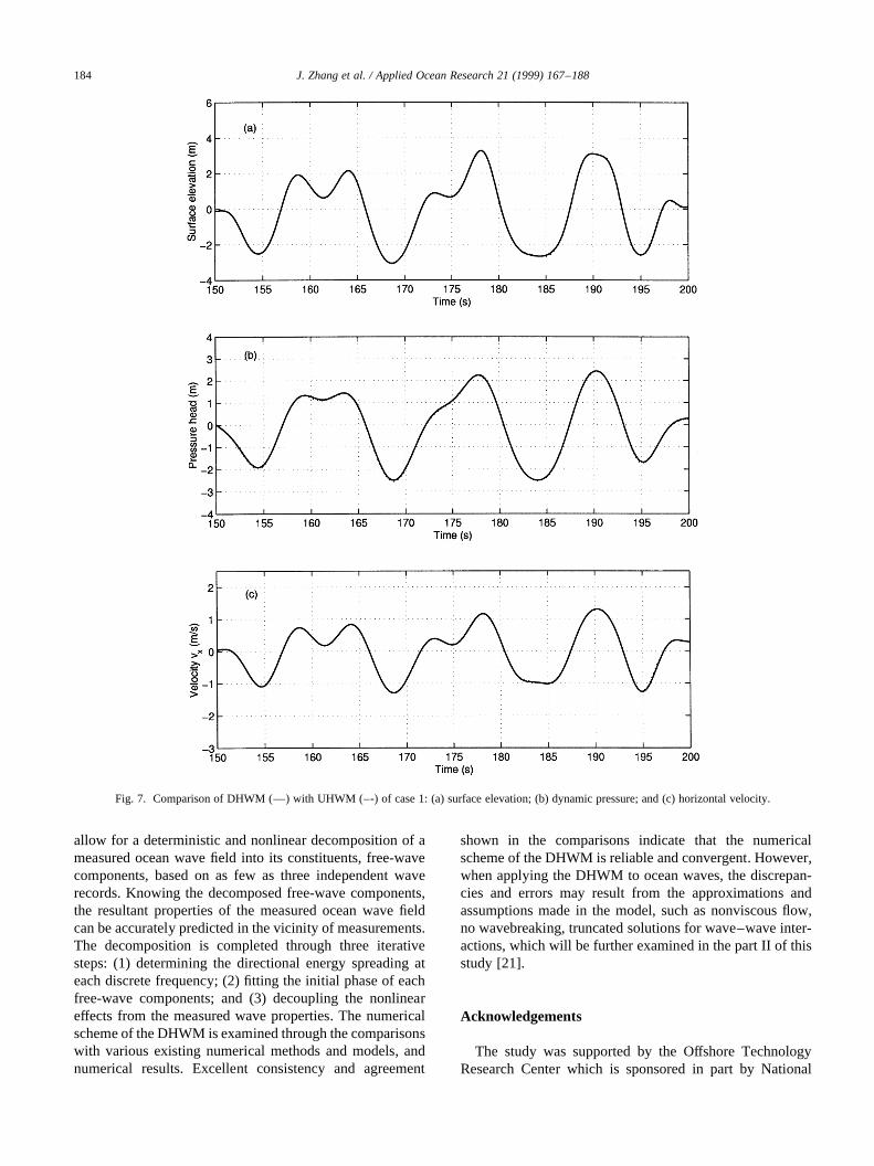
A unidirectional (long-crested) wave field is a specialcase of a directional wave field, in which all wave compo-nents are propagating in the same direction. Since theUHWM has been validated against laboratory measure-ments [4], the DHWM is examined against the UHWM in


Fig. 4. Comparison of predictedx-direction horizontal velocity as a function of depth, the phase modulation solution (-X-), the conventional solutions of firstorder (I–) and up to second order (II–), and long-wave velocity only (-× -).

predicting the properties of unidirectional irregular wavetrains. In the first case, the nominal maximum wave steep-ness of a unidirectional irregular wave train is 0.18, which isdefined as the product of the half of the maximum waveheight (within the elevation time series considered) andthe wavenumber at the peak frequency. The water depth is145.0 m. The amplitudes and initial phases of free-wavecomponents used as input for the computation of resultantwave properties are similar to those obtained in the decom-position of the measurements described in [21; Section 2 ofPart II]. All free-wave components advance in the directionof x-axis. Both UHWM and DHWM are used to compute theresultant surface elevation about 10 m downstream of themeasurement, and the pressure and velocity at the samehorizontal location but 8.25 m below the still water level.

As shown in Fig. 7, the predictions of these two models arein excellent agreement.

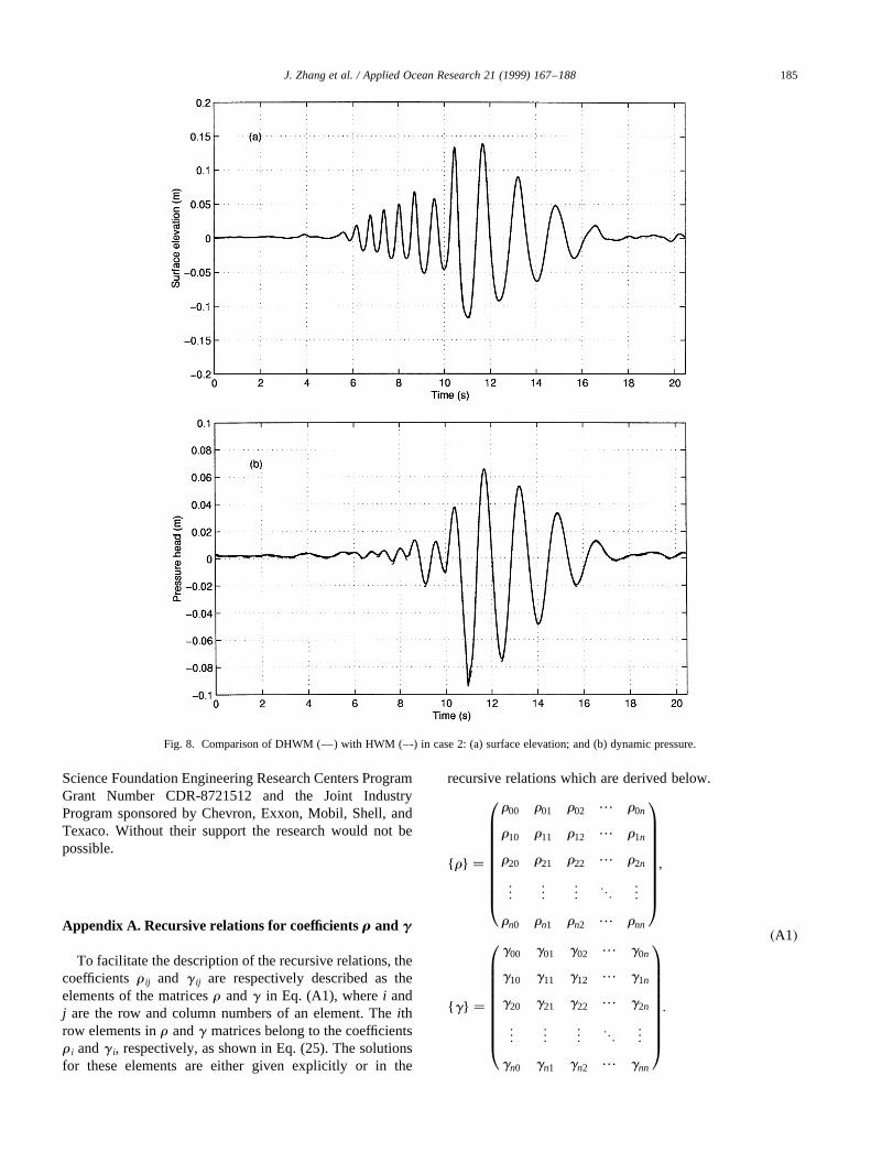
In the second case, we consider a unidirectional transientwave train with extremely steep crests, which eventuallyleads to wave breaking [37]. The nominal maximum steep-ness of the wave train is 0.2344. The water depth is 0.90 m.When the free-wave components of the transient wave trainare given, the surface elevation atx � 0 and the dynamicpressure at the same horizontal location but 25 cm below thestill water level are calculated using the two models. Fig. 8shows that the results calculated using the two models arealmost identical. These comparisons indicate that thenonlinear wave formulations in the DHWM and UHWMare consistent in computing unidirectional irregularwaves.


Fig. 5. Comparison between the conventional and phase modulation solutions for two free-wave interactione1� 0.20,e l � 0.139: (a) short-wave elevation atleading-order (—), up to the second order (–-) of the conventional solution and (-X-) of the phase modulation solution; (b) leading-order short-wave elevation(—) and the second-order conventional solution (–-). The horizontal coordinate,Q1/2p, is normalized long-wave phase.

6.3. Decomposition of a synthetic wave field

The numerical tests are also designed to examine whetheror not the iteration in the DHWM decomposition is able torender unique and convergent free-wave components basedon a few point wave records. For that purpose, given theamplitudes, directional angles and initial phases of a set offree-wave components, a synthetic short-crested wave fieldcan be numerically simulated using the superposition part ofthe DHWM. The resultant wave properties include thecontributions from these free-wave components as well astheir interactions. They are recorded at three fixed points asa function of time. These point records are then used as theinput for the decomposition of the synthetic wave field usingthe DHWM. The comparison between the decomposed free-wave components and those used as the input to the simula-tion of the synthetic wave field may divulge whether or notthe numerical scheme is able to decompose a wave fieldaccurately.

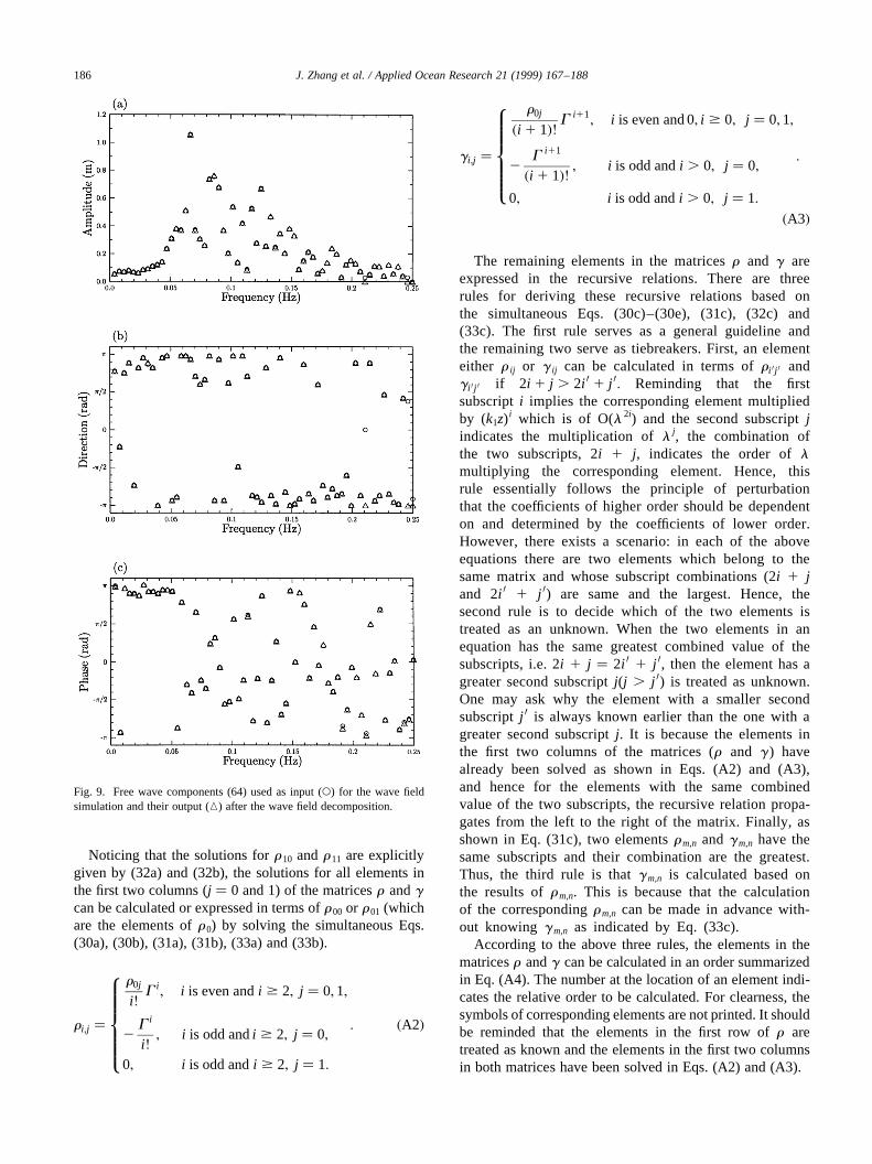
Many tests of synthetic wave fields have been made. Forbrevity, selected below is a short-crested wave field simu-lated based on a set of free-wave components similar tothose of a real wave field described in [21; Section 2 ofPart II]. The synthetic wave field consists of 64 discretefrequencies and a single representative free-wave compo-nent at each discrete frequency is used. The water depth in145 m. The amplitudes, directional angles and initial phasesof the free-wave components used as the input to the super-position part of the DHWM are shown as (o) in Fig. 9. The

resultant wave elevation at the origin and two orthogonalhorizontal velocity components at the same horizontal posi-tion but 8.53 m below the still water level are calculated as afunction of time. The records at these three points are thenused as the input to the decomposition part of the DHWM.Based on these three records, the amplitudes, directionalangles and initial phases of the free-wave components canbe obtained and shown as (K) in Fig. 9. The comparisonsshow that the decomposed free-wave components arealmost coincident with those used as the input. There aresome small discrepancies for the wave components of verylow energy. The discrepancies may result from two sources.First, because the amplitudes of these components are toosmall, the observed errors result in insignificant errors ofresultant properties which can be smaller than the prescribederror tolerance. Secondly, as pointed out by Jeffery [38], thecovariance matrix used in the EMLM can be singular if theinput data are from a single realization. The singularity canbe avoided by adding incoherent noises of small magnitudeto the matrix [38]. This operation might slightly affect thedecomposed results. Excellent agreement was also observedwhen the surface elevations at three fixed points were usedas the input to the decomposition [39].

7. Conclusion

The DHWM is developed for the study of short-crestedirregular ocean waves. The innovation of the DHWM is to


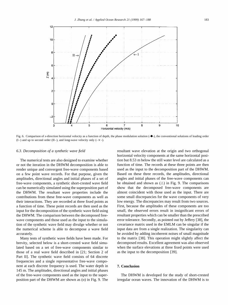
Fig. 6. Comparison ofx-direction horizontal velocity as a function of depth, the phase modulation solution (-X-), the conventional solutions of leading order(I–) and up to second order (II–), and long-wave velocity only (-× -).

allow for a deterministic and nonlinear decomposition of ameasured ocean wave field into its constituents, free-wavecomponents, based on as few as three independent waverecords. Knowing the decomposed free-wave components,the resultant properties of the measured ocean wave fieldcan be accurately predicted in the vicinity of measurements.The decomposition is completed through three iterativesteps: (1) determining the directional energy spreading ateach discrete frequency; (2) fitting the initial phase of eachfree-wave components; and (3) decoupling the nonlineareffects from the measured wave properties. The numericalscheme of the DHWM is examined through the comparisonswith various existing numerical methods and models, andnumerical results. Excellent consistency and agreement

shown in the comparisons indicate that the numericalscheme of the DHWM is reliable and convergent. However,when applying the DHWM to ocean waves, the discrepan-cies and errors may result from the approximations andassumptions made in the model, such as nonviscous flow,no wavebreaking, truncated solutions for wave–wave inter-actions, which will be further examined in the part II of thisstudy [21].

Acknowledgements

The study was supported by the Offshore TechnologyResearch Center which is sponsored in part by National


Fig. 7. Comparison of DHWM (—) with UHWM (–-) of case 1: (a) surface elevation; (b) dynamic pressure; and (c) horizontal velocity.

Science Foundation Engineering Research Centers ProgramGrant Number CDR-8721512 and the Joint IndustryProgram sponsored by Chevron, Exxon, Mobil, Shell, andTexaco. Without their support the research would not bepossible.

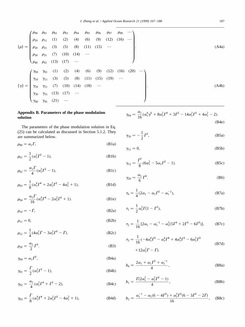
Appendix A. Recursive relations for coefficientsr andg

To facilitate the description of the recursive relations, thecoefficientsr ij and g ij are respectively described as theelements of the matricesr andg in Eq. (A1), wherei andj are the row and column numbers of an element. Theithrow elements inr andg matrices belong to the coefficientsr i andg i, respectively, as shown in Eq. (25). The solutionsfor these elements are either given explicitly or in the

recursive relations which are derived below.

{r} �

r00 r01 r02… r0n

r10 r11 r12… r1n

r20 r21 r22… r2n

..

. ... ..

.]

..

.

rn0 rn1 rn2… rnn

0BBBBBBBBBB@

1CCCCCCCCCCA;

{g} �

g00 g01 g02… g0n

g10 g11 g12… g1n

g20 g21 g22… g2n

..

. ... ..

.]

..

.

gn0 gn1 gn2… gnn

0BBBBBBBBBB@

1CCCCCCCCCCA:

�A1�


Fig. 8. Comparison of DHWM (—) with HWM (–-) in case 2: (a) surface elevation; and (b) dynamic pressure.

Noticing that the solutions forr10 andr11 are explicitlygiven by (32a) and (32b), the solutions for all elements inthe first two columns (j � 0 and 1) of the matricesr andgcan be calculated or expressed in terms ofr00 or r01 (whichare the elements ofr0) by solving the simultaneous Eqs.(30a), (30b), (31a), (31b), (33a) and (33b).

ri;j �

r0j

i!G i

; i is even andi $ 2; j � 0;1;

2G i

i!; i is odd andi $ 2; j � 0;

0; i is odd andi $ 2; j � 1:

:

8>>>>><>>>>>:�A2�

gi;j �

r0j

�i 1 1�! Gi11

; i is even and 0; i $ 0; j � 0; 1;

2G i11

�i 1 1�! ; i is odd andi . 0; j � 0;

0; i is odd andi . 0; j � 1:

:

8>>>>><>>>>>:�A3�

The remaining elements in the matricesr and g areexpressed in the recursive relations. There are threerules for deriving these recursive relations based onthe simultaneous Eqs. (30c)–(30e), (31c), (32c) and(33c). The first rule serves as a general guideline andthe remaining two serve as tiebreakers. First, an elementeither r ij or g ij can be calculated in terms ofri 0 j 0 andgi 0 j 0 if 2i 1 j . 2i 0 1 j 0: Reminding that the firstsubscripti implies the corresponding element multipliedby (k1z)

i which is of O(l 2i) and the second subscriptjindicates the multiplication ofl j, the combination ofthe two subscripts, 2i 1 j, indicates the order oflmultiplying the corresponding element. Hence, thisrule essentially follows the principle of perturbationthat the coefficients of higher order should be dependenton and determined by the coefficients of lower order.However, there exists a scenario: in each of the aboveequations there are two elements which belong to thesame matrix and whose subscript combinations (2i 1 jand 2i 0 1 j 0) are same and the largest. Hence, thesecond rule is to decide which of the two elements istreated as an unknown. When the two elements in anequation has the same greatest combined value of thesubscripts, i.e. 2i 1 j � 2i 0 1 j 0, then the element has agreater second subscriptj(j . j 0) is treated as unknown.One may ask why the element with a smaller secondsubscriptj 0 is always known earlier than the one with agreater second subscriptj. It is because the elements inthe first two columns of the matrices (r and g ) havealready been solved as shown in Eqs. (A2) and (A3),and hence for the elements with the same combinedvalue of the two subscripts, the recursive relation propa-gates from the left to the right of the matrix. Finally, asshown in Eq. (31c), two elementsrm,n andgm,n have thesame subscripts and their combination are the greatest.Thus, the third rule is thatgm,n is calculated based onthe results ofrm,n. This is because that the calculationof the correspondingrm,n can be made in advance with-out knowing gm,n as indicated by Eq. (33c).

According to the above three rules, the elements in thematricesr andg can be calculated in an order summarizedin Eq. (A4). The number at the location of an element indi-cates the relative order to be calculated. For clearness, thesymbols of corresponding elements are not printed. It shouldbe reminded that the elements in the first row ofr aretreated as known and the elements in the first two columnsin both matrices have been solved in Eqs. (A2) and (A3).


Fig. 9. Free wave components (64) used as input (W) for the wave fieldsimulation and their output (K) after the wave field decomposition.

Appendix B. Parameters of the phase modulationsolution

The parameters of the phase modulation solution in Eq.(25) can be calculated as discussed in Section 5.1.2. Theyare summarized below.

r00 � a1G; �B1a�

r01 � 12�a2

1G2 2 1�; �B1b�

r02 � a1G

4�a2

1G2 2 1�; �B1c�

r03 � 18�a4

1G4 1 2a2

1G2 2 4a2

1 1 1�; �B1d�

r04 � a1G

16�a4

1G4 2 2a2

1G2 1 1�: �B1e�

r10 � 2G; �B2a�

r11 � 0; �B2b�

r12 � 14�4a2

1G 2 3a21G

3 2 G�: �B2c�

r20 � a1

2G3

: �B3�

g00 � a1G2; �B4a�

g01 � G

2�a2

1G2 2 1�; �B4b�

g02 � a1

4�a2

1G4 1 G2 2 2�; �B4c�

g03 � G

8�a4

1G4 1 2a2

1G2 2 4a2

1 1 1�; �B4d�

g04 � a1

16�a4

1g6 1 8a2

1G4 1 3G2 2 14a2

1G2 1 4a2

1 2 2�:�B4e�

g10 � 212G2

; �B5a�

g11 � 0; �B5b�

g12 � G2

8�6a2

1 2 5a1G2 2 1�: �B5c�

g20 � a1

6G4

: �B6�

t0 � 14�2a1 2 a1G

2 2 a211 �; �B7a�

t1 � 12a2

1G�1 2 G2�; �B7b�

t2 � 116�2a1 2 a21

1 2 a31�5G4 1 2G3 2 6G2��; �B7c�

t3 � 116�24a4

1G5 2 a4

1G4 1 4a4

1G3 2 6a2

1G3

112a21G 2 G�:

�B7d�

b0 � 2a1 1 a1G2 1 a21

1

4; �B8a�

b1 � G�2a21 2 a2

1G2 2 1�

4; �B8b�

b2 � a211 2 a1�6 2 4G2�1 a3

1G2�6 2 3G2 2 2G�

16; �B8c�


{r} �

r00 r01 r02 r03 r04 r05 r06 r07 r08…

r10 r11 �1� �2� �4� �6� �9� �12� �16� …

r20 r21 �3� �5� �8� �11� �15� …

r30 r31 �7� �10� �14� …

r40 r41 �13� �17� …

0BBBBBBBBB@

1CCCCCCCCCA; �A4a�

{g} �

g00 g01 �1� �2� �4� �6� �9� �12� �16� �20� …

g10 g11 �3� �5� �8� �11� �15� �19� …

g20 g21 �7� �10� �14� �18� …

g30 g31 �13� �17� …

g40 g41 �21� …

0BBBBBBBBB@

1CCCCCCCCCA: �A4b�

b3 � 116�a5

1G5 1 4a4

1G5 1 a4

1G4 2 4a4

1G3 2 2a3

1G3

16a21G

3 2 12a21G 1 a1G 1 G�: (B8d)

References

[1] Funke ER, Mansard EPD. On the meaning of phase spectra. In:Proceedings of the International Symposium on Hydrodynamics inOcean Engineering, The Norwegian Institute of Technology, Norway,1981, p. 49–69.

[2] Zhang J, Chen L, Ye M, Randall RE. Hybrid wave model for unidir-ectional irregular waves. Part I. Theory and numerical scheme. ApplOcean Res 1996;18:77–92.

[3] Torum A, Gudmestad OT. Water wave kinematics. NATO ASISeries, Series E: Applied Science, 178. Dordrecht: Kluwer Academic,1989.

[4] Spell CA, Zhang J, Randall RE. Hybrid wave model for unidirectionalirregular waves. Part II. Comparison with laboratory measurements.Appl Ocean Res 1996;18:93–110.

[5] Zhang J, Meza Conde E, Yang J. Wave elevation based on the pres-sure measurements. Texas A&M University, COE Rep. No. 352, 1996

[6] Borgman LE. Irregular ocean waves: kinematics and forces. The Sea,Ocean Engineering Science, Part A, 9. New York: Wiley, 1990 p. 121.

[7] Tick LJ. A non-linear random model of gravity waves I. J Maths andMech 1959;8:643–652.

[8] Weber BL, Barrick DE. On the nonlinear theory for gravity waves onthe ocean’s surface. Part I: Derivations. J Phys Oceanog 1977;7:3–7.

[9] Komen GJ. Nonlinear contributions to the frequency spectrum ofwind-generated water waves. J Phys Oceanogr 1980;10:779–790.

[10] Masuda A, Kuo Y, Mitsuyasu H. On the dispersion relation of randomgravity waves. Part 1 Theoretical framework. J Fluid Mech1979;92:717–730.

[11] Mitsuyatsu H, Kuo Y, Masuda A. On the dispersion relation ofrandom gravity waves. Part 2 An experiment. J Fluid Mech1979;92:731–749.

[12] Herbers THC, Guza RT. Wind wave nonlinearity observed at the seafloor, Part I: forced wave energy. J Phys Oceanogr1991;21(12):1740–1761.

[13] Herbers THC, Guza RT. Wind-wave nonlinearity observed on theseafloor: Part II: Wavenumbers and third-order statistics. J PhysOceanog 1992;22(5):489–504.

[14] Sand SE. Three-dimensional deterministic structure of ocean waves.Institute of Hydrodynamics and Hydraulic Engineering, Series Paper24, 177 pp., Technical University of Denmark, 1979.

[15] Schaffer HA, Hyllested P. Analysis of multidirectional waves usingdeterministic decomposition, in: International symposium on waves-physical and numerical modeling, UBC, Vancouver, Canada, Vol. 2,1994, p. 911–920.

[16] Zhang J, Hong K, Yue DKP. Effects of wavelength ratio on wavemodeling. J Fluid Mech 1993;248:107–127.

[17] Prislin I, Zhang J, Seymour RJ. Deterministic decomposition of deepwater short-crested irregular gravity waves. J Geophy Res1997;102(C6):12677–12688.

[18] Su MY, Green AW. Experimental studies of strong nonlinear

interactions of deep-water gravity waves. In: Phillips OM, Hassel-mann K, editors. Wave dynamics and radio probing of the oceansurface, New York: Plenum, 1981. p. 231.

[19] Phillips OM. Surface wave physics-a survey. Flow Research Report,145, 91 pp. Flow Research Co. Division of Flow Industries, Inc.,Kent, WA, 1979.

[20] Hasselmann K. On the non-linear energy transfer in a gravity-wavespectrum. Part 1. General theory. J Fluid Mech 1962;12:481–500.

[21] Zhang J, Prislin I, Yang J, Wen J. Deterministic wave model for short-crested ocean waves: Part II. Comparison with laboratory and fieldmeasurements. Appl Ocean Res 1999;21:191–208.

[22] Isobe M, Kondo K, Horikawa K. Extension of MLM for estimatingdirectional wave spectrum. Proc. Symposium on Description andModeling of Directional seas, Paper No. A-6, Technical Universityof Denmark, 1984, p. 1–15.

[23] van Heteren J, Keijser H, Schaap B. Comparison wave directionalmeasuring systems. Appl Ocean Res 1988;10(3):128–143.

[24] Goda Y. Directional wave spectrum and its application in coastalengineering. In: Proceedings of the International Conference onHydrodynamics, China Ocean Press. 1994, p. 9–18.

[25] Herbers THC, Guza RT. Estimation of directional wave spectrafrom multicomponent observations. J Phys Oceanogr1990;20:1703–1724.

[26] Hashimoto N, Nagai T, Asai T. Extension of the maximum entropyprinciple method for directional wave spectrum estimation, CoastalEngineering 1994, ASCE, 1994, p. 232–246.

[27] Press WH, Teukolsky SA, Vatterling WT, Flannery BP. Numericalrecipes infortran: the art of scientific computing, 2. Cambridge:Cambridge University Press, 1992 963 pp.

[28] Longuet-Higgins MS, Stewart RW. Changes in the form of shortgravity waves on long waves and tidal currents. J Fluid Mech1960;8:565–583.

[29] Zhang J, Melville WK. Evolution of weakly nonlinear shortwaves riding on long gravity waves. J Fluid Mech1990;214:321–346.

[30] Chen L, Zhang J. On interaction between intermediate-depth longwaves and deep-water short waves. Ocean Engng 1998;25(6):395–423.

[31] Longuet-Higgins MS. Resonant interactions between two trains ofgravity waves. J Fluid Mech 1962;12:321–332.

[32] Hsu JRC, Tsuchiya Y, Silvester R. Third-order approximation toshort-crested waves. J Fluid Mech 1979;90:179–196.

[33] Hong K. Nonlinear interactions between directional dual componentwaves in deep water. PhD Thesis, Texas A&M University, 1993.

[34] Phillips OM. The dispersion of short wavelets in presence of domi-nant long wave. J Fluid Mech 1981;107:465–485.

[35] Longuet-Higgins MS. The propagation of short surface gravity waveson longer gravity waves. J Fluid Mech 1987;177:293–306.

[36] Zhang J, Randall RE, Spell CA. On wave kinematics approximatemethods. In: Proceedings of the 23rd Offshore Technology Confer-ence, Houston, Texas, 1991.

[37] Zhang J, Conde EM, Seymour RJ. Experimental studies on energydissipation in breaking waves. In: Proceedings of the 7th ISOPE, vol.3, 1997, p. 178–183.

[38] Jefferys ER. Comparison of three methods for calculation of direc-tional spectra. In: Proceedings of the 5th International OMAE Sympo-sium, ASME, Tokyo, vol. 1, 1986, p. 45–50.

[39] Prislin I. Nonlinear deterministic decomposition of short-crestedocean wave. PhD Thesis, Texas A & M University, 1996.


Date post:	06-Aug-2015
Category:	Engineering
Upload:	sompong-bangyeekhan
View:	45 times
Download:	1 times