1

Sentiment Classification on Steam ReviewsRohan Bais, Pasal Odek, Seyla Ou

I. INTRODUCTION

Sentiment Analysis is a machine-learning topic that has beenperformed frequently and exhausted quickly in many scenarios,given the high demand to understanding sentiment within abody of any general text. However, language is not always laidout in such a straightforward fashion. In real world examples,people do not simply echo or spam highly polarizing positiveand negative words to make it easy for machine learning tacticsto classify; human-written text is much more nuanced thansimply that. In day-to-day life, text has personality written intoit: text can have a mixture of conflicting feelings that maymake it hard to classify into one definite category, text canhave cultural references or memes embedded into them thatmake it easy for humans but hard for computers to spot thesentiment, and most troublesome of all, text can have sarcasmimbued over it that can sometimes even trick humans intothinking theyre genuine reactions. Since real-world text is moresubtle and nuanced than a simple positive and negative binaryclassification, we wanted to test the bounds of binary sentimentclassification with positive and negative labels, using a morehip and modern-lingo based review system as a resource, sowe turned to the Steam gaming platform’s review system.

Steam is a multi-billion dollar distributed gaming platformthat acts as a third-party medium to sell games online anddownload them. Generally, the user-base for this platform hasbeen young (it ranges from 18 to 30), so naturally, because itis a game-review platform and the base is somewhat young,the culture around Steam is built on sarcasm, memes, and wit.

With trickier texts such as Steam game reviews, we hopedto build a binary sentiment classifier to peg reviews as positiveand negative, seeing if it would work with the languagesubtleties explained earlier. The input to the sentiment classifieris a plain-text review attached with the metadata surroundingthe review such as percent of people who found the reviewhelpful, funny, and number of hours the reviewer played.Using these inputs, we used the approaches of SVMs, LogisticRegression, Multinomial Naive Bayes, Turney’s unsupervisedphrase-labeling algorithm, and a lexicon-based baseline.

II. RELATED WORK

Despite the problem not being a completely novel one,various people have been working on sentiment classificationto see if it can overcome language subtleties like mentionedearlier and achieve perfect accuracy, not even missing outsarcastic reviews. Pang and Lee tried sentiment classificationof IMDB reviews but tried varying the feature set to includeunigrams, bigrams, and part-of-speech tagging, to improvethe generic unigram method as the go-to feature set. Theresults were promising, as bigrams kept track of some contextof the words that the bag-of-words model did not, although

the part-of-speech tagging provided no valuable increase inaccuracy[1]. Another approach built off of the approach hereby Pak and Paroubek, and used a more generic n-gramsmodel, with n up to 3, to try and fully capture the contextof the situation and included some pivotal features such asemoticons and used these for the SVM and Naive Bayesapproaches. Emoticons, like “:)” and “:(” are generally strongindicators of sentiment as they are brief and very rarely dothey matter so much in contexts like individual words do.With these changes, they improved upon Pang and Lee’swork [2]. Other methods, such as the models from Prusaand Dittman, rely more on the unigram model directly butadd weighting schemes such as TF-IDF (term-frequency andinverse-document-frequency) and hand-writing a couple ofrules with additional weighting when words are italicized orbolded [4]. The results have also been proven to do betterthan the standard unigram model, as unigrams just weigh ona basis of term frequency without consideration of uniquenessof a particular word and how pivotal it is. It better achievedaccuracy than the previous two approaches, but still failed onclassifying sarcastic reviews.

Others people, such as Turney, tried to approach this ina different regard with unsupervised learning and phrasaldetection. Turney used POS-tagging to extract phrasesand determined a semantic orientation by calculating co-occurrence with a phrase and a positive and with the phraseand a negative word (e.g. ”excellent” and ”poor”) [3]. Thenhe averages the scores of all phrases in a review to seethe sentiment. This has proven somewhat successful as hisextraction gets key phrases out and ignores the fat and notuseful text in a lot of reviews, but it lacks context sometimesand classifies incorrectly when mistaking a description of amovie as an actual sentiment. State-of-the-art is geared moretowards recursive or convolutional neural networks since theyeliminate high-bias and high variance. A paper from Ren andZhang shows that recursive neural networks combined withword2vec word embeddings, which turns words into vectorsthat are close if the words are similar and far apart if not,achieves a very high accuracy, with the only flaws being itsinability to detect sarcasm [5]. Our approach shares muchin common with these mentioned approaches despite thedifference in datasets, we use Turney’s algorithm and we relynot only on words and word-weighting as features, but wealso use features outside of the individual words in the review,like hours played or percent found review helpful, to betterachieve accuracy during sentiment classification and avoid thesame pitfalls of not detecting sarcasm without context.

2

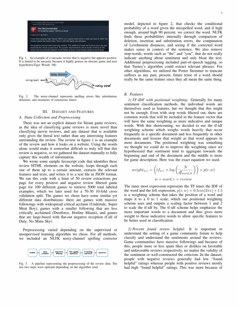
Fig. 1. An example of a sarcastic review that is negative but appears positive.It is hinted to be sarcastic because it highly praises an obscure game and useshyperboles(Tiger Woods ’08)

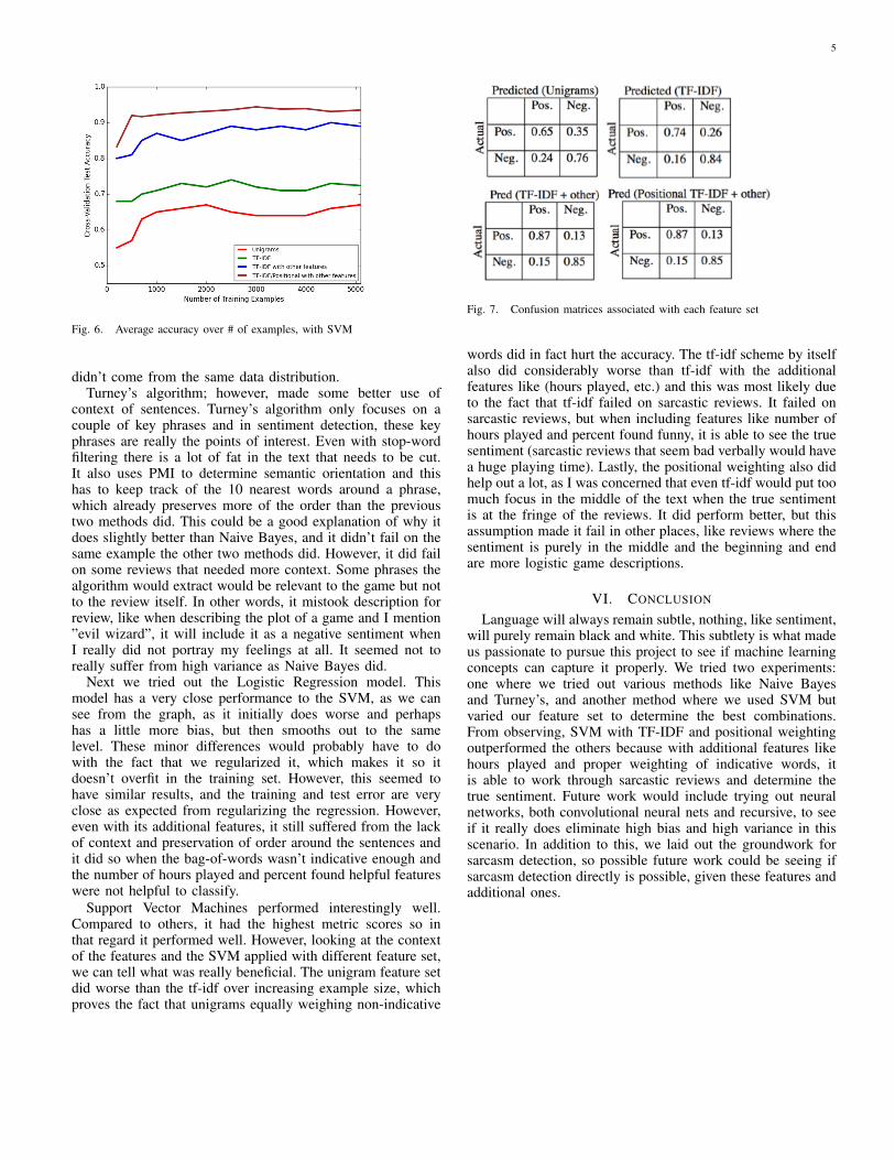
Fig. 2. The noisy-channel represents spelling errors like substitution,deletions, and insertions of extraneous letters

III. DATASET AND FEATURES

A. Data Collection and Preprocessing

There was not an explicit dataset for Steam game reviews,as the idea of classifying game reviews is more novel thanclassifying movie reviews, and any dataset that is availableonly gives the literal text rather than any interesting featuressurrounding the review. The review in figure 1 is an exampleof the review and how it looks on a website. Using the wordsalone would make it somewhat difficult to truly tell that thisreview is negative, so we gathered the dataset manually to fullycapture this wealth of information.

We wrote some sample Javascript code that identifies thesereview HTML elements on the website, loops through eachone of them up to a certain amount, extracts the relevantfeatures and texts, and writes it to a text file in JSON format.We ran this code with a limit of 50 review extractions perpage for every positive and negative review filtered gamepage for 100 different games to retrieve 5000 total labeledexamples, which we later used for a 70-30 10-fold crossvalidation split. The games we chose have some similar yetdifferent data distributions: there are games with massivefollowings with widespread critical acclaim (Undertale, SuperMeat Boy), games with a smaller following that are lesscritically acclaimed (Dustforce, Hotline Miami), and gamesthat are large-based with flat-out negative reception (Call ofDuty, No Mans Sky)

Preprocessing varied depending on the supervised orunsupervised learning algorithm we chose. For all methods,we included an NLTK noisy-channel spelling corrector

Fig. 3. A pipeline representing the preprocessing of the review data. Thelast two steps were optional depending on the algorithm used

model, depicted in figure 2, that checks the conditionalprobability of a word given the misspelled word, and if highenough, around high 90 percent, we correct the word. NLTKfinds these probabilities internally through comparison ofdeletion, insertion and substitution errors, the computationof Levehnstein distances, and seeing if the corrected wordmakes sense in context of the sentence. We also removestop-words, words such as “the” and “you”, that do not reallyindicate anything about sentiment and only bloat the text.Additional preprocessing included part-of-speech tagging, sothat Turney’s algorithm could extract relevant phrases. Forother algorithms, we utilized the Porter Stemmer to truncatesuffixes as any past, present, future tense of a word shouldreally be the same feature since they all mean the same thing.

B. Features

1) TF-IDF with positional weighting: Generally for manysentiment classification methods, the individual words arethemselves used as features, but we thought that this mightnot be enough. Even with stop words filtered out, there arecommon words that will be included in the feature vector thatwill have the same weighting as more indicative and uniquewords. With this shortcoming, we decided to use the tf-idfweighting scheme which weighs words heavily that occurfrequently in a specific document and less frequently in otherdocuments and lessens that weight as that word appears inmore documents. The positional weighting was somethingwe thought we could do to improve the weighting since wehypothesized that sentiment tend to aggregate towards thebeginning and end of the document and the middle is morefor game description. Here was the exact equation we used:

weightw,r

=

✓tf

w,r

⇥ log

✓N

dfword,N

◆◆⇥ p(r, w)

w = word, r = review

The inner most expression represents the TF times the IDF ofthe word and the left expression, p(r, w) = 0.5cos(2⇡x)+1.5is a weighting scheme that takes the position of a word andmaps it to a 0 to 1 scale, which our positional weightingscheme uses and outputs a scaling factor between 1 and 2to scale the tf-idf by. The tf-idf scheme helps emphasize themore important words to a document and thus gives moreweight to those indicative words to allow specific features tobe better used in classification.

2) Percent found review helpful: It is important tounderstand the setting of a game community forum to helpclassify and understand the sentiments around the reviews.Game communities have massive followings and because ofthis, people more or less spam likes or dislikes on favorableand unfavorable reviews respectively, no matter the validity ofthe sentiment or well-constructed the criticism. In the dataset,people with negative reviews generally had low “foundhelpful” ratings whereas people with positive reviews mostlyhad high “found helpful” ratings. This was more because of

3

the massive fan-base of the game liking and disliking positiveand negative reviews respectively, so it could be used as adistinguishing feature.

3) Percent found review funny: Funny and humorousreviews are something that can be tied to both positive andnegative reviews (in our dataset, positive funny reviews tendedto be more self- deprecatory about “crying while playingan emotional game” whereas negative reviews lambastwith ridiculous analogies and lengthy rants). The sameecho-chamber phenomenon described earlier appears here aswell: positive reviews were found more funny and negativereviewers hit more soft spots and were generally found lessfunny, even if the negative review was somewhat humorous.

4) Number of hours played: The number of hours playedalso tends to show a trend for positive and negative reviews.Positive reviews will generally have the users playing upwardsfrom 20 to 1000 hours (depending on how replay-able thegame is). Negative reviews, on the other hand, will have fewerthan 10 hours played, mostly due to the fact that if someonefound a review negative, he or she wouldnt want to spend toomuch time playing and reliving negative experiences, whichkeeps the hour count small.

IV. METHODS

A. Lexicon Score Aggregation

Our baseline consisted of just simply utilizing a dictionaryof positive and negative words and simply just aggregating thetotal counts and checking which . We thought to try this asthis was a simple method to implement and we wanted to seewhere exactly it would fail on subtleties in language and howit would fare relative to the other methods above this baseline.

B. Multinomial Naive Bayes

For the next method, we thought we would try Naive Bayes,since that is the next step up or is usually a baseline. It wasused with the features being a “bag-of-words” (only counts ofunigrams, no order particularly) approach combined with stopword filtering. It breaks down a review using the unigrams asfeatures and after training and computing conditional proba-bilities of words appearing in positive and negative reviews, ituses these probabilities directly to classify any test data

cpredicted

= argmaxc

P (r|c)P (c)

cpredicted

= argmaxc

P (c)⇥

Y

w

i

2r

P (wi

|c)!

It tries to find the probability of a certain class given thereview P (c|r) and uses Bayes Rule to get the first equation. Weare interested in the class that maximizes the probability, andthe second equation’s product comes from the independenceassumption that the features (words) are independent of eachother and can be split into a product of probabilities. We triedthis method out to see the shortcomings of Naive Bayes and tosee if the independence assumption or other types of sentencestrips the classifier up.

C. Modified Turney’s Algorithm

We wanted to see how an semi-supervised learning algo-rithm would compare to the more supervised-heavy algorithmsthat we would use later on. Turney’s algorithm works byextracting key phrases. Phrases follow a certain set of rulescountable by hand. A phrase consists of two words where:the first is an adjective and the second is a noun, the two areboth adjectives, the first is an noun followed the second as anadjective, or the first is a adverb and second is a adjective.As an example the first pattern can be exemplified with thephrase “great game” (adjective followed by noun) and thefourth pattern can be exemplified with the phrase “absolutelyterrifying” (adverb followed by noun).

Given the reviews, in a training and test split, it takes thereviews of the training data, extracts all of the phrases out ofthese reviews and the first 10 words surrounding the phrases.It also keeps track of the all positive and negative words in thetraining data reviews using the same dictionary in the lexiconmethod as a set of top words. When classifying a review in thetest scenario, it extracts all the phrases in the review, checks thetraining set if that phrase appeared (if not ignore it) and thenit calculates the point-wise mutual information (PMI) betweenthat phrase and all the positive and negative words found inthe set of top words and computes the semantic orientationby taking all of the pointwise mutual information of positivewords and subtracting them by pointwise mutual informationof negative words. Using the semantic orientation of a phrase,it aggregates the semantic orientation of all of the review’sphrases and uses that number to determine if a review ispositive or negative (positive average semantic orientation ispositive, negative is negative). Here are the equations:

PMI(p, w) =# of times p appears with w

# of times w appears

SO(p, r) =X

w2r+

PMI(p, w)�X

w2r�

PMI(p, w)

The first equation just simply counts co occurrence bychecking how many times a word appears with a phraseand dividing it by how many times a word appears. Thesecond equation, describing the semantic orientation, worksby calculating by summing all of the PMIs in r+, whichis all positive words in a review r, and summing all thePMIs in r�, which is all negative words in r and subtractingthe two. It differs from Turney’s original slightly in thatTurney’s only used the words “excellent” and “poor” tocheck semantic orientation, which we felt like wasn’t enough.Thus we generalized it to work with all positive and negativewords in reviews, though it becomes more expensive doing so.

D. Logistic Regression

Logistic Regression is a Generalized Linear Model that isused widely for multi-class classification. It works by trying tofit the sigmoid function, g = 1

1+e

�x

, to the individual labeledpoints (0 for negative, 1 for positive in a binary classification

4

example). It has a hypothesis function h(x) = g(✓Tx) where xis the feature vector of an example and ✓ is a weighting vectorlearned, which represents the probability that x is classified aspositive (similarly, 1 � h(x) is the probability x is negative).It primarily trains itself using these data points by using astochastic gradient ascent update rule:

✓j

:= ✓j

+ ↵(yi � h(x))xi

j

where ↵ is the learning rate to affect how quickly theprogram converges and how it steps. After the weights aregiven, we simply compute the hypothesis function.

E. Linear SVM

Linear SVM is a method that creates a classifier (a vector)that separates the two labeled point, at least in the binaryclassification case. Geometrically given the two types of points,circles and x’s, in a space, it tries to maximize the minimumdistance from one of the points to the place. In other words, itmaximizes the margin. Although kernel tricks can be appliedto make the data more linearly separable, we did not thinkit was necessary as we have high-dimensional feature vectorsthat are most of the time linearly separable. The optimizationproblem the SVM tries to solve is below:

min�,w,b

1

2||w||2

s.t.yi(wTx+ b) � 1, i = 1, 2, ...m

It tries to find the w to satisfy the maximum margin problemand satisfy the separability constraint.

In addition to using all of these methods, we wanted totest our feature set using the same method to judge how thefeatures fared with classification capability, so we used LinearSVM for this task as well as comparing the algorithm’sclassification capability to other methods mentioned earlier.

V. EXPERIMENTS AND RESULTS

Since we are performing binary sentiment classification,we chose accuracy, precision and F1-score as metrics ofperformance, as well as the original test and training setaccuracies.

Our experiments mainly delved into two types: one exper-iment was to test how the algorithms themselves fare againsteach other over an increasing training set size. The methods tocompare include the baseline, Naive Bayes, Logistic Regres-sion, and Turney’s Algorithm. The second set of experimentswas to check what exactly was the ideal feature set and howfeature selection affected the same metrics (precision, accuracyand recall). For both of these experiments, we performed 10-fold cross validation with a 70-30 percent training-test datasplit as we wanted to see how a moving window of trainingand test sizes affect the metrics and see whether or not that tellsus about the distribution and similarity/differences amongst thedata points. The training-test split was approximately around3500 reviews in the training set and 1500 reviews in the testset for each of the 10 folds

Fig. 4. Average accuracy over # of examples

Fig. 5. The average metrics for each of the 5 methods

For our first experiment, testing the various methods againsteach other, we performed the cross-validation and reported theaverage results in figure 4. In figure 5 we show how the algo-rithms perform over a variable number of learning examples,starting from 200 going all the way to 5000 examples.

Our baseline, as expected under-performed, with an averageaccuracy of 59 percent. The errors for this method sproutedwhen it couldn’t find the subtleties in the sentences. For manypositive examples, there were reviews saturated with positivewords and fewer negative words but it was not able to graspthe concluding sentiment, despite being much shorter thanthe rest of the review, is the true sentiment. As an example,“I thought the prequel was fantastic and great, but this ishorrendous” starts off positively and ends negatively, but ourmethod would see more positive words than negative wordsand label it positive.

Naive Bayes was also seemed to have fared better as itperformed better over more training examples. This method;however, suffered many of the short comings the baseline had.Again, because of the independence assumption, the words’order is lost. Texts can have the same or nearly the same bagof word feature set and still have opposite meanings. It doesn’tfare well against the earlier example as well, as it will findfantastic and great to have high probabilities for a positivelabel, but it should have really focused more on the statementafter the “but” transition. Looking at the graph and the table,it had a higher variance and this probably was because withjust the bag of words feature, the training and test data split

5

Fig. 6. Average accuracy over # of examples, with SVM

didn’t come from the same data distribution.Turney’s algorithm; however, made some better use of

context of sentences. Turney’s algorithm only focuses on acouple of key phrases and in sentiment detection, these keyphrases are really the points of interest. Even with stop-wordfiltering there is a lot of fat in the text that needs to be cut.It also uses PMI to determine semantic orientation and thishas to keep track of the 10 nearest words around a phrase,which already preserves more of the order than the previoustwo methods did. This could be a good explanation of why itdoes slightly better than Naive Bayes, and it didn’t fail on thesame example the other two methods did. However, it did failon some reviews that needed more context. Some phrases thealgorithm would extract would be relevant to the game but notto the review itself. In other words, it mistook description forreview, like when describing the plot of a game and I mention”evil wizard”, it will include it as a negative sentiment whenI really did not portray my feelings at all. It seemed not toreally suffer from high variance as Naive Bayes did.

Next we tried out the Logistic Regression model. Thismodel has a very close performance to the SVM, as we cansee from the graph, as it initially does worse and perhapshas a little more bias, but then smooths out to the samelevel. These minor differences would probably have to dowith the fact that we regularized it, which makes it so itdoesn’t overfit in the training set. However, this seemed tohave similar results, and the training and test error are veryclose as expected from regularizing the regression. However,even with its additional features, it still suffered from the lackof context and preservation of order around the sentences andit did so when the bag-of-words wasn’t indicative enough andthe number of hours played and percent found helpful featureswere not helpful to classify.

Support Vector Machines performed interestingly well.Compared to others, it had the highest metric scores so inthat regard it performed well. However, looking at the contextof the features and the SVM applied with different feature set,we can tell what was really beneficial. The unigram feature setdid worse than the tf-idf over increasing example size, whichproves the fact that unigrams equally weighing non-indicative

Fig. 7. Confusion matrices associated with each feature set

words did in fact hurt the accuracy. The tf-idf scheme by itselfalso did considerably worse than tf-idf with the additionalfeatures like (hours played, etc.) and this was most likely dueto the fact that tf-idf failed on sarcastic reviews. It failed onsarcastic reviews, but when including features like number ofhours played and percent found funny, it is able to see the truesentiment (sarcastic reviews that seem bad verbally would havea huge playing time). Lastly, the positional weighting also didhelp out a lot, as I was concerned that even tf-idf would put toomuch focus in the middle of the text when the true sentimentis at the fringe of the reviews. It did perform better, but thisassumption made it fail in other places, like reviews where thesentiment is purely in the middle and the beginning and endare more logistic game descriptions.

VI. CONCLUSION

Language will always remain subtle, nothing, like sentiment,will purely remain black and white. This subtlety is what madeus passionate to pursue this project to see if machine learningconcepts can capture it properly. We tried two experiments:one where we tried out various methods like Naive Bayesand Turney’s, and another method where we used SVM butvaried our feature set to determine the best combinations.From observing, SVM with TF-IDF and positional weightingoutperformed the others because with additional features likehours played and proper weighting of indicative words, itis able to work through sarcastic reviews and determine thetrue sentiment. Future work would include trying out neuralnetworks, both convolutional neural nets and recursive, to seeif it really does eliminate high bias and high variance in thisscenario. In addition to this, we laid out the groundwork forsarcasm detection, so possible future work could be seeing ifsarcasm detection directly is possible, given these features andadditional ones.

6

VII. REFERENCES

[1] Lee, Lillian, et al. “Thumbs up? Sentiment ClassificationUsing Machine Learning Techniques.” 2001 Cornell CSJournal.

[2] Pak, Alexander et al. “Twitter as a Corpus for SentimentAnalysis and Opinion Mining” January 2010, DBLP Journal

[3] Prusa, Joseph et al. “Impact of Feature SelectionTechniques for Tweet Sentiment Classification” May 2013,Florida Aritifical Intelligence Society Conference

[4] Turney, Peter “Thumbs Up or Thumbs Down?Semantic Orientation Applied to Unsupervised Classificationof Reviews” July 2002, Association for ComputationalLinguistics

[5] Ren, Yafeng, Zhang, Yue “Context-Sensitive TwitterSentiment Classification Using Neural Network” January 11,2016 AAAI publication

VIII. CONTRIBUTIONS

Rohan: Implemented tf-idf weighting scheme, as well ascross validation and the various SVM methods and Turney’s.Helped write up the final write-up.

Seyla: Implemented the Naive Bayes method with cross-validation as well and helped with the poster and write-upmostly. Proposed and determined feature sets for testing aswell.

Pascal: Implemented the baseline and wrote the htmlparsing code to extract each of the 50 positive and 50 negativereviews from the 100 games we chose. Also helped write thisup.