100
| Date post: | 21-Dec-2015 |
| Category: |
Documents |
| View: | 214 times |
| Download: | 0 times |

2
Recall Dynamic Programming and 1 || Tj
Algorithm 3.4.4.
Dynamic programming procedure: recursively the optimal solution forsome job set J starting at time t is determined from the optimal solutionsto subproblems defined by job subsets of S*S with start times t*t .
J(j, l, k) contains all the jobs in a set {j, j+1, ... , l} with processing time pk
V( J(j, l, k) , t) total tardiness of the subset under an optimal sequenceif this subset starts at time t

3
Initial conditions:V(, t) = 0V( { j }, t ) = max (0, t + pj - dj)
Recursive conditions:
)))(,)',,1'((
))(,0max(
),)',',(((min),),,((
'
''
k
kk
CklkJV
dC
tkkjJVtkljJV
where k' is such thatpk' = max ( pj' | j' J(j, l, k) )
Optimal value function is obtained forV( { 1,...,n }, 0 )

4
Recall Example
jobs 1 2 3 4 5pj 121 79 147 83 130dj 260 266 266 336 337
( (1, 3, 3), 0 ) 81 ( (4, 5, 3), 347 )
({1,2,...,5},0) min ( (1, 4, 3), 0 ) 164 ( (5, 5, 3), 430 )
( (1, 5, 3), 0 ) 294 ( , 560 )
V J V J
V V J V J
V J V

5
V( J(1, 4, 3) , 0)=0 achieved with the sequence 1, 2, 4 and 2, 1, 4
jobs 1 2 4 pj 121 79 83 dj 260 266 336
( , 0 ) 0 ( (2,4,1), 121 )
( (1,4,3),0) min ( (2,2,1), 0 ) 0 ( (4,4,1), 200 )
( (1,4,1), 0 ) 23 ( , 283 )
V V J
V J V J V J
V J V
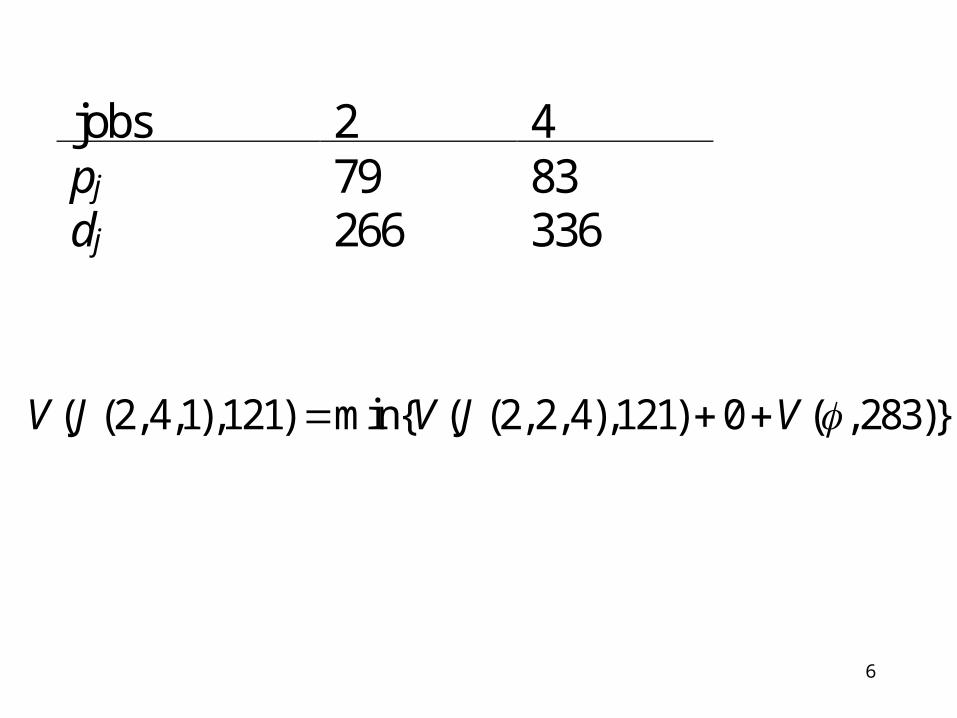
6
jobs 2 4 pj 79 83 dj 266 336
( (2,4,1),121) min{ ( (2,2,4),121) 0 ( , 283)}V J V J V
7
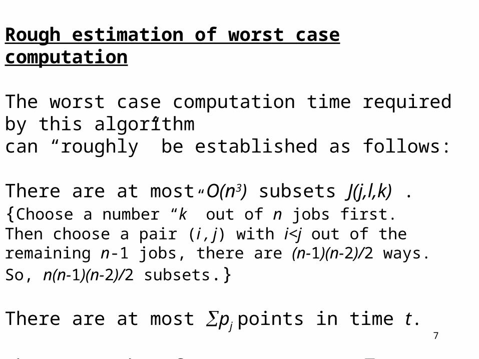
Rough estimation of worst case computation
The worst case computation time required by this algorithm can “roughly” be established as follows:
There are at most O(n3) subsets J(j,l,k) . {Choose a number “k” out of n jobs first. Then choose a pair (i , j) with i<j out of the remaining n-1 jobs, there are (n-1)(n-2)/2 ways. So, n(n-1)(n-2)/2 subsets.}
There are at most pj points in time t.
There are therefore at most O(n3 pj) recursive equationsto be solved in the dynamic programming algorithm.

8
As each recursive equation takes O(n) time, the overallRunning time of the algorithm is bounded by O(n4 pj), which is clearly a polynomial in n. (Pseudopolynomial).
Pseudopolynomial O(n4 pj)
Suppose there are two scheduling problems 1 || Tj with the same number of jobs n, and same due dates.
Does it make sense to say the one with larger completion time will have a larger upper bound of computational time ?

9
Lemma Consider the problem 1 || Tj with n jobs. The jobs can be scheduled with zero total tardiness if and only ifthe EDD schedule results in a zero total tardiness.
Proof
Since the smallest possible value 1 || Tj can take is zero, if the EDD schedule results in a zero total tardiness, then these n jobs can be schedule with zero total tardiness.
( )
( ) Suppose, without loss of generality, ,and jobs can be scheduled so that 1 || Tj =0,i.e. Tj=0 for all j=1,2,…,n.
1 2 nd d d
Let j < k , so . j kd d
10
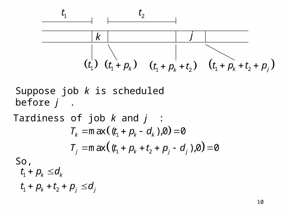
1t 1 kt p 1 2kt p t
k j
1 2k jt p t p
1t 2t
Tardiness of job k and j :
1max ( ),0 0k k kT t p d
1 2max ( ),0 0j k j jT t p t p d
Suppose job k is scheduled before j .
1
1 2
k k
k j j
t p d
t p t p d
So,
11
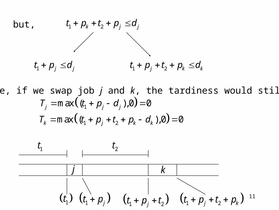
1 2k j jt p t p d but,
1 j jt p d 1 2j k kt p t p d
Therefore, if we swap job j and k, the tardiness would still be 0
1t 1 jt p 1 2jt p t
j k
1 2j kt p t p
1t 2t
1max ( ),0 0j j jT t p d
1 2max ( ),0 0k j k kT t p t p d
12
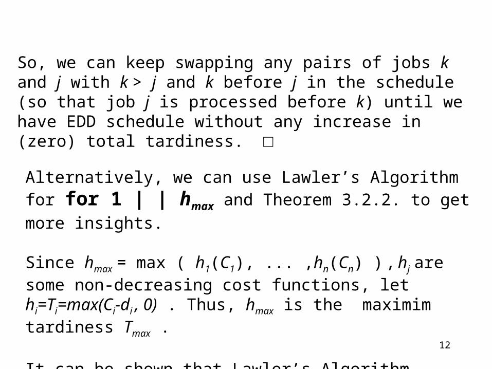
So, we can keep swapping any pairs of jobs k and j with k > j and k before j in the schedule (so that job j is processed before k) until we have EDD schedule without any increase in (zero) total tardiness. □
Alternatively, we can use Lawler’s Algorithm for for 1 | | hmax
and Theorem 3.2.2. to get more insights.
Since hmax = max ( h1(C1), ... ,hn(Cn) ) , hj are some non-decreasing cost functions, let hi=Ti=max(Ci-di , 0) . Thus, hmax is the maximim tardiness Tmax .
It can be shown that Lawler’s Algorithm results in the EDD rule.

13
Step 1.
J = JC = {1,...,n}k = n
Step 2.
Let j* be such that
CCC Jj
jjJjJj
jj phph min*
Place j* in J in the k-th order positionDelete j* from JC
Step 3.
If JC = then Stopelse k = k - 1
go to Step 2
Recall Lawler’s Algorithm for 1 | | hmax

14
1 || Tmax is the special case of the 1 | prec | hmax
where hj = Tj=max( Cj-dj , 0).
Lawler’s algorithm results in the schedule that orders jobs in increasing order of their due dates - earliest due date first rule (EDD)
1d
1T
2d
2T
3d
3T
Thus, the EDD rule minimize maximum tardiness Tmax . Therefore,zero total tardiness Tj =0 implies zero maximum tardiness Tmax =0 implies EDD rule results in zero tardiness.
15
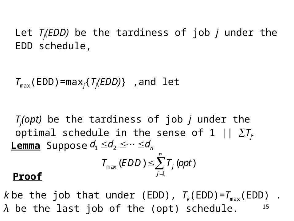
Lemma Suppose
max1
( ) ( )n
jj
T EDD T opt
Proof
Let k be the job that under (EDD), Tk(EDD)=Tmax(EDD) .Let λ be the last job of the (opt) schedule.
Let Tj(EDD) be the tardiness of job j under the EDD schedule,
Tmax(EDD)=maxj{Tj(EDD)} ,and let
Tj(opt) be the tardiness of job j under the optimal schedule in the sense of 1 || Tj.
1 2 nd d d

16
Case I : If λ ≤ k .
Case II : If k < λ and there exists δ ( δ < k ) such that under (opt), job δ is scheduled after job k but before λ. Let δ* be the last of such a job in (opt) schedule so that no other job
with a job number larger than k is scheduled after δ* .
Case III : If k < λ , and no job with a job number larger than k is scheduled after job k in (opt).
δ*k λ> k
k λ> k
Three cases to consider:

17
Case I : If λ ≤ k , so dλ≤dk , then
1
( )n
k jj
T EDD T opt
1
( ) max ,0n
jj
T opt p d
1
max ,0k
j kj
p d
1
max ,0n
j kj
p d
kT EDD

18
Case II : If k < λ and there exists δ ( δ < k ) such that under (opt), job δ is scheduled after job k but before λ. Let δ* be the last of such a job in (opt) schedule so that no other job
with a job number larger than k is scheduled after δ* .
δ*k λ> k
* *:_ _ _
_ _ _ *
( ) max ,0jj all jobs before
and include
T opt p d
1
max ,0k
j kj
p d
*
1
max ,0k
jj
p d
kT EDD
1
( )n
k jj
T EDD T opt
19
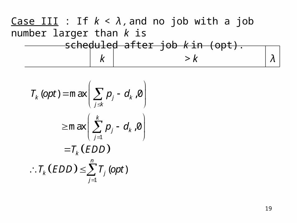
Case III : If k < λ , and no job with a job number larger than k is scheduled after job k in (opt).
k λ> k
( ) max ,0k j kj k
T opt p d
1
max ,0k
j kj
p d
kT EDD
1
( )n
k jj
T EDD T opt
20
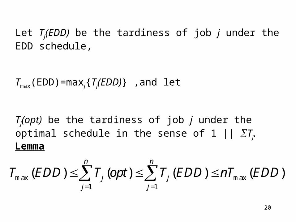
max max1 1
( ) ( ) ( ) ( )n n
j jj j
T EDD T opt T EDD nT EDD
Lemma
Let Tj(EDD) be the tardiness of job j under the EDD schedule,
Tmax(EDD)=maxj{Tj(EDD)} ,and let
Tj(opt) be the tardiness of job j under the optimal schedule in the sense of 1 || Tj.

21

22
23

24
Lemma
Suppose sequence S minimize problem 1 || Tj with processing times pj and due dates dj. Then, sequence S also minimize the rescaled scheduling problem with provessing times Kpi and rescaled due dates Kdj for some positive constant K .
Proof Consider the total tardiness :
1 1 1
max{ ,0} max{ ,0}n n n
i j i j jj i j i j
Kp Kd K p d K T
Clearly, minimizing total tardiness and 1
n
jj
T
1
n
jj
K T
are equivalent.

25
Lemma
Consider two scheduling problems of minimizing total tardiness. The first problem has processing times pi and due dates di, whereas, the second problem has processing time qi and due dates di. Let pi qi for all i.
The optimal total tardiness of the first problem is less than or equal to the optimal total tardiness of the second problem.
Proof Consider the total tardiness of optimal solution
to the second problem:
1 1
max{ ,0} max{ ,0}n n
i j i jj j
q d p d

26Note that,

27

28

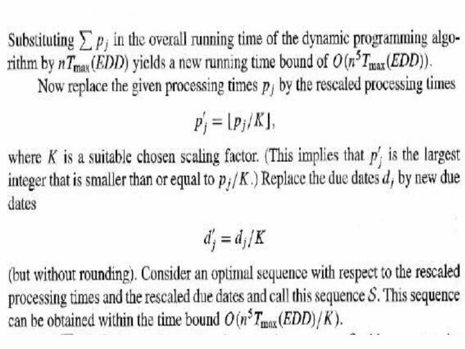
29
30
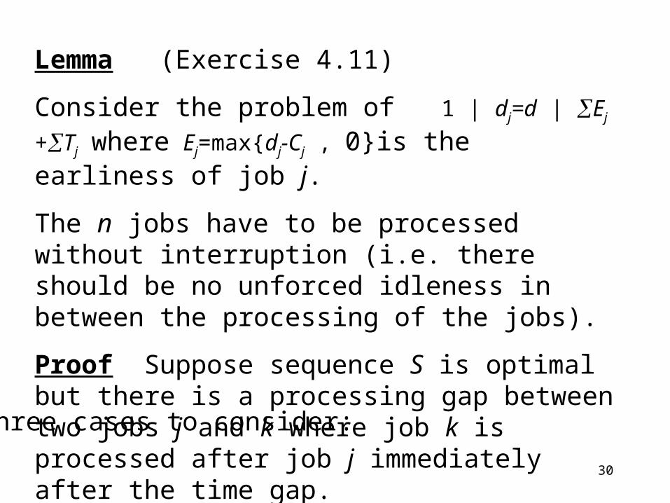
Lemma (Exercise 4.11)
Consider the problem of 1 | dj=d | Ej +Tj where
Ej=max{dj-Cj , 0}is the earliness of job j.
The n jobs have to be processed without interruption (i.e. there should be no unforced idleness in between the processing of the jobs).
Proof Suppose sequence S is optimal but there is a processing gap between two jobs j and k where job k is processed after job j immediately after the time gap.
Three cases to consider:

31
Case I : If the time gap is beyond d.
j k
d
time gap
Let J1 be the set of jobs processed before the time gap, and J2 be the set of jobs processed after the time gap.
Let t0 be the time where first job starts, and t1 be the length of the time gab.

32
Case II : If the time gap is before d.
j k
d
time gap

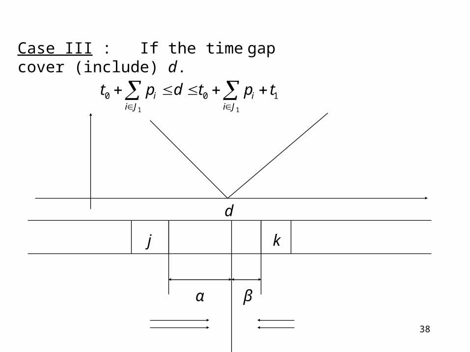
33
Case III : If the time gap cover (include) d.
j k
d
time gap
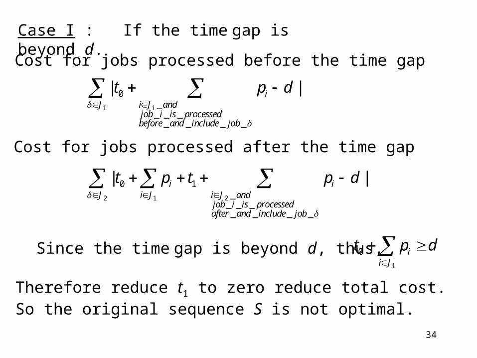
34
Case I : If the time gap is beyond d.
1 1
0_
_ _ __ _ _ _
| |iJ i J and
job i is processedbefore and include job
t p d
Cost for jobs processed before the time gap
2 1 2
0 1_
_ _ __ _ _ _
| |i iJ i J i J and
job i is processedafter and include job
t p t p d
Cost for jobs processed after the time gap
1
0 ii J
t p d
Since the time gap is beyond d, thus,
Therefore reduce t1 to zero reduce total cost. So the original sequence S is not optimal.

35
j k
d
2 1 2
0_
_ _ __ _ _ _
| 0 |i iJ i J i J and
job i is processedafter and include job
t p p d
Cost for jobs processed after the time gap

36
Case II : If the time gap is before d.
2 1 2
0 1_
_ _ __ _ _ _
| |i iJ i J i J and
job i is processedafter and include job
t p t p d
1 1
0_
_ _ __ _ _ _
| |iJ i J and
job i is processedbefore and include job
t p d
Cost for jobs processed before the time gap
Cost for jobs processed after the time gap
Since the time gap is before d, thus,
Therefore increase t0 to (t0 +t1) and reduce t1 to zero will reduce total cost. So the original sequence S is not optimal.
1
0 1ii J
t p t d

37
j k
d
1 1
0 1_
_ _ __ _ _ _
| ( ) |iJ i J and
job i is processedbefore and include job
t t p d
Cost for jobs processed before the time gap (decreased)
2 1 2
0 1_
_ _ __ _ _ _
| ( ) 0 |i iJ i J i J and
job i is processedafter and include job
t t p p d
Cost for jobs processed after the time gap (remain unchanged)
38
Case III : If the time gap cover (include) d.
1 1
0 0 1i ii J i J
t p d t p t
j k
d
α β

39
Therefore increase t0 to (t0 +α) and reduce t1 to zero will reduce total cost. So the original sequence S is not optimal.
Hence, increase t0 to (t0 +α) would make1
0 ii J
t p d
j k
d
By contradiction of the 3 cases, the original sequence S is not optimal !!!□
40
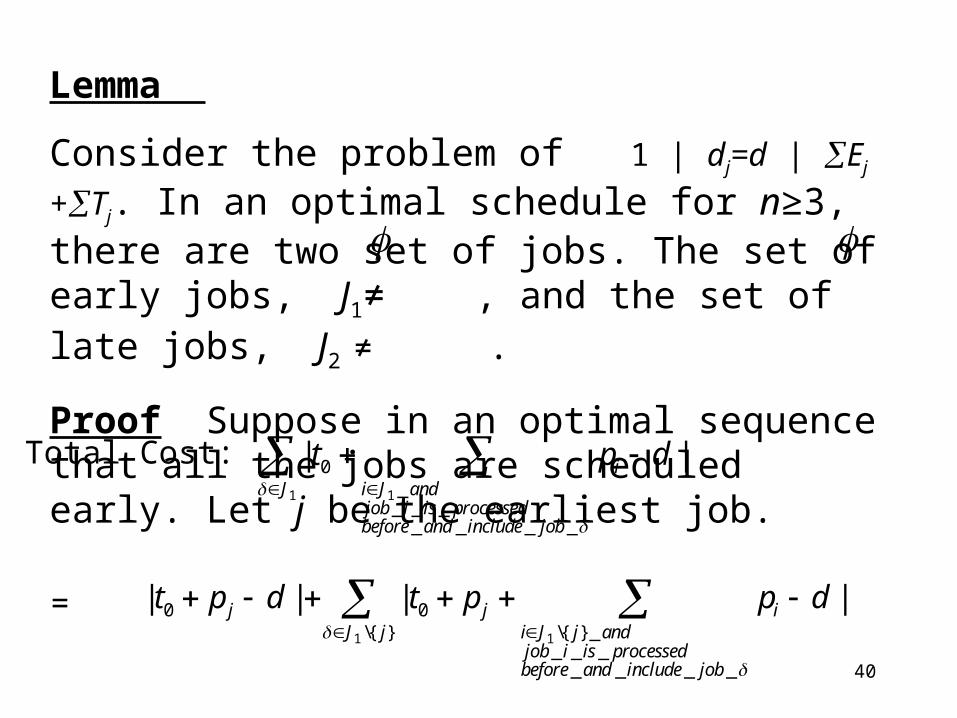
Lemma
Consider the problem of 1 | dj=d | Ej +Tj. In an optimal schedule for n≥3, there are two set of jobs. The set of early jobs, J1≠ , and the set of late jobs, J2 ≠ .
Proof Suppose in an optimal sequence that all the jobs are scheduled early. Let j be the earliest job.
1 1
0_
_ _ __ _ _ _
| |iJ i J and
job i is processedbefore and include job
t p d
Total Cost:
1 1
0 0\{ } \{ }_
_ _ __ _ _ _
| | | |j j iJ j i J j and
job i is processedbefore and include job
t p d t p p d
=

41
Suppose d-t0 > 2pj. Thus, |t0+pj-d| > |pj|.
Now, re-schedule job j to start at d, and the starting time for all
other jobs remain unchanged.So for the remaining jobs, J1 becomes J1\{j}, and t0 becomes t0+pj.
d
jj
J1

42
1 1
0\{ } \{ }_
_ _ __ _ _ _
| | | ( ) |j j iJ j i J j and
job i is processedbefore and include job
d p d t p p d
Total Cost :
1 1
0\{ } \{ }_
_ _ __ _ _ _
| | | ( ) |j j iJ j i J j and
job i is processedbefore and include job
p t p p d
=
=
So, by contradiction, the original sequence that all jobs are early is not optimal.
What if d-t0 < 2pj ?

43
Similarly, we can show by contradiction that, if the original sequence consists of all jobs that are late, is not optimal. □
d
j
j

44
Lemma 4.2.1
Consider the problem of 1 | dj=d | Ej +Tj. In an optimal schedule, the early jobs, set J1, are scheduled according to LPT, and the late jobs, set J2 , are scheduled according to SPT.
Proof (Exercise 4.12)
Observe that all jobs in J1 do not contribute to Tj and all jobs in J2 do not contribute to Ej . Let |J1| be the number of jobs in J1 and |J2| be the number of jobs in J2.
Also, observe that for J1, the only cost contribution is:
Ej = max{dj-Cj , 0}= (|J1|d)-( Cj), since all jobs are early.

45
Similarly, for J2, the only cost contribution is:
Tj = max{Cj - dj, 0}= ( Cj)-(|J2|d) since all jobs are late.
Thus, for all late jobs (all jobs in J2), we try to minimize the total flow Cj.
Hence, among all jobs in J2, we use SPT (Theorem 3.1.1).
What is left is to show that among all early jobs (all jobs in J1), the LPT rule minimize (- Cj), the negative total flow, or, LPT maximize the total flow. This is left as an exercise to you.

46
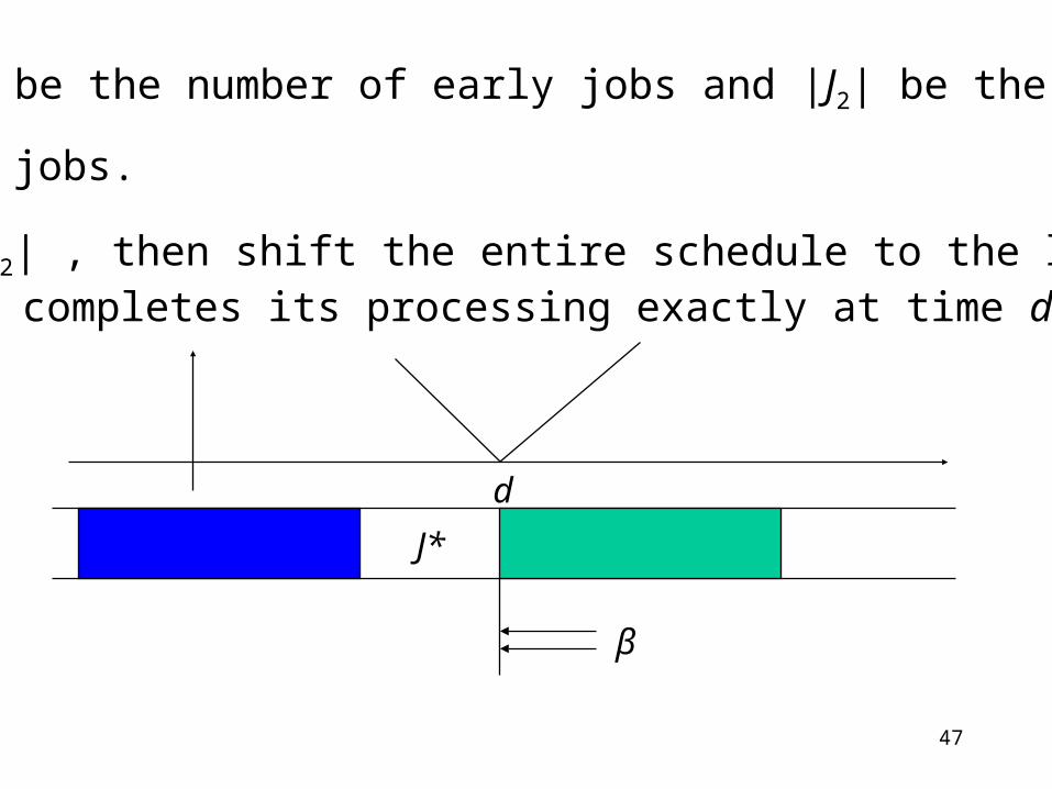
Lemma 4.2.2 Consider 1 | dj=d | Ej +Tj. In an optimal schedule, there exists an optimal schedule in which one job is completed exactly at time d.
Proof Suppose there are no such optimal schedule. There exists one job that starts its processing before d and completes it processing after d. Call this job j*.
J*
d
α β
47
Let |J1| be the number of early jobs and |J2| be the number
of late jobs.
If |J1| < |J2| , then shift the entire schedule to the left such that job j* completes its processing exactly at time d.
J*
d
β

48
The total tardiness: decreased by β [ |J2|-1]
The total earliness: increased by β |J1|
But |J1| < |J2|, i.e. |J1| ≤ |J2|-1, thus, β |J1| ≤ β [|J2|-1],so the total cost is decreased.
If |J1| > |J2| , then shift the entire schedule to the right such that job j* starts its processing exactly at time d.
J*
d
α
49
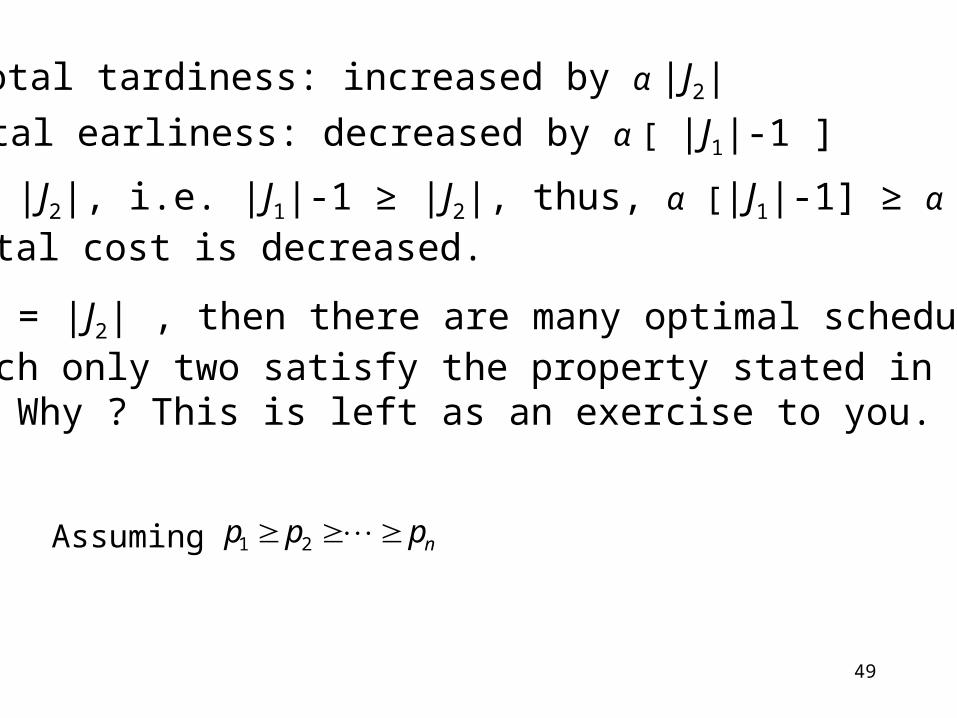
The total tardiness: increased by α |J2|
The total earliness: decreased by α [ |J1|-1 ]
But |J1| > |J2|, i.e. |J1|-1 ≥ |J2|, thus, α [|J1|-1] ≥ α |J2|,so the total cost is decreased.
If |J1| = |J2| , then there are many optimal schedules,of which only two satisfy the property stated in the Lemma. Why ? This is left as an exercise to you.
1 2 np p p Assuming

50
Assuming 1 2 np p p
51
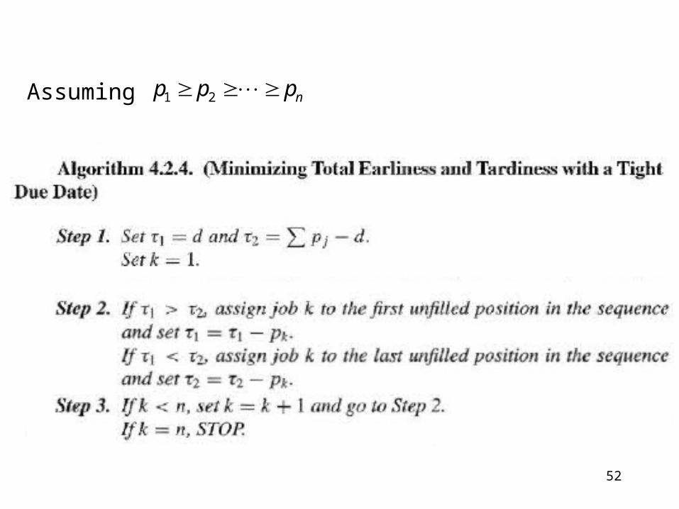
52
Assuming 1 2 np p p

53
d jp
1 2
The length of the blue band is depicting 1
and the length of the yellow band is depicting 2
Can be negative
54
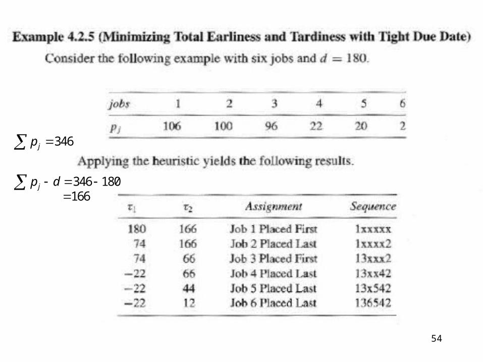
346jp
346 180jp d 166
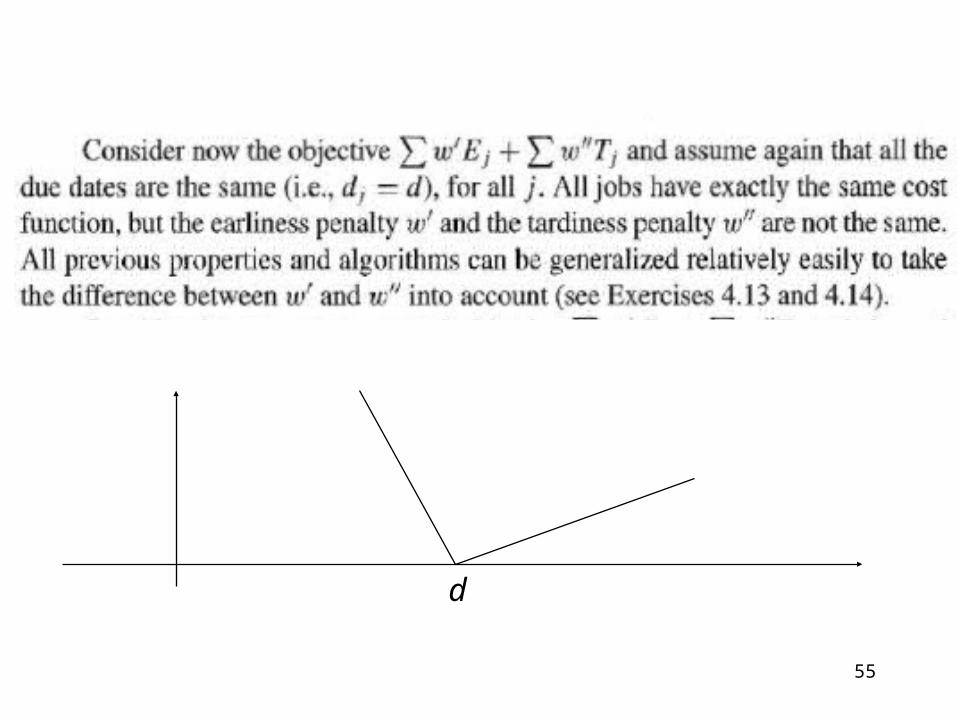
55
d
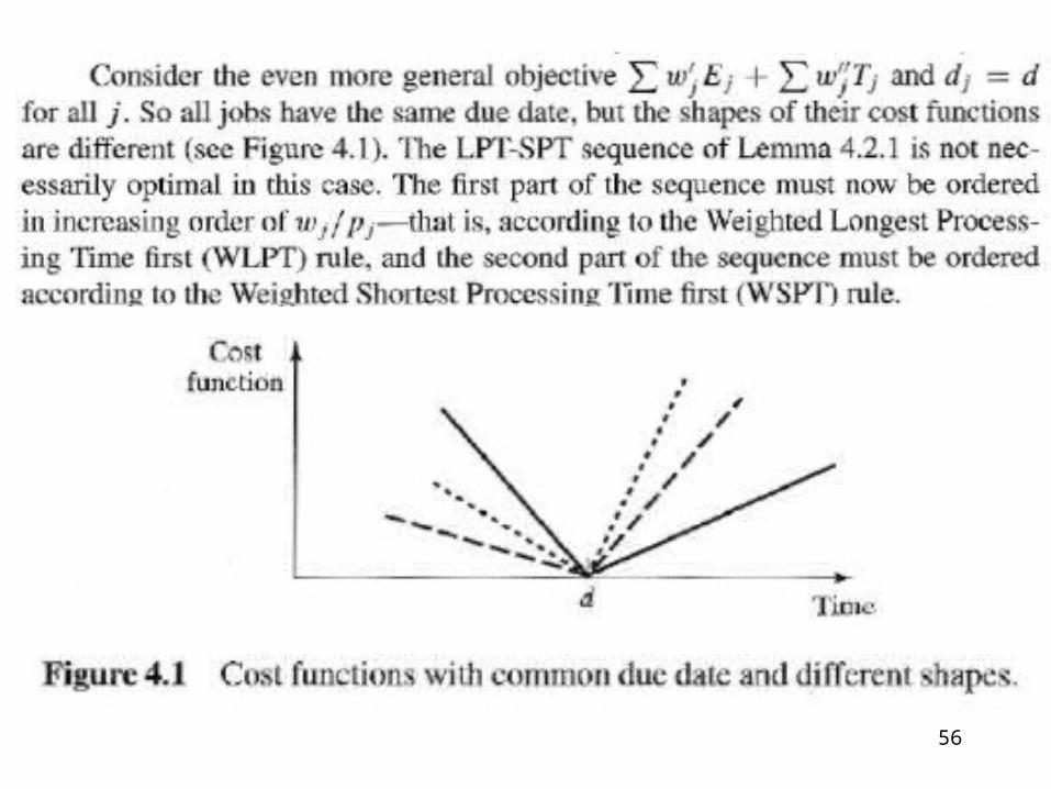
56

57

58
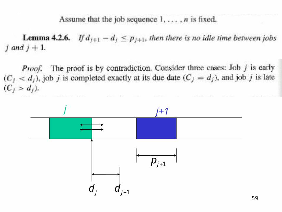
59
j+1j
1jp
1jd jd

60

611jd jd 2jd
2jp 1jp jp

62

63

64

65
Clearly,
Let
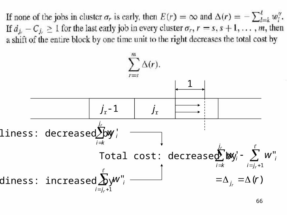
66
jr
1
jr-1
Earliness: decreased by
1
' "r
r
j
i ii k i j
w w
Tardiness: increased by1
"r
ii j
w
Total cost: decreased by
'rj
ii k
w
( )rj
r

67
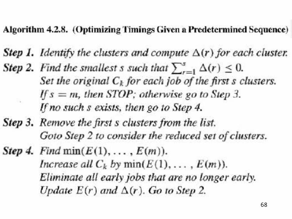
68

69

70

71

72
Sequence-Dependent Setup Problems
An algorithm which gives an optimal schedule with the minimum makespan with sequence-dependent setup times
1 | Sjk | Cmax
Single machine: rj=0, no sequence dependent setup times j
jpCmax
However, solving 1 | Sjk | Cmax is NP hard
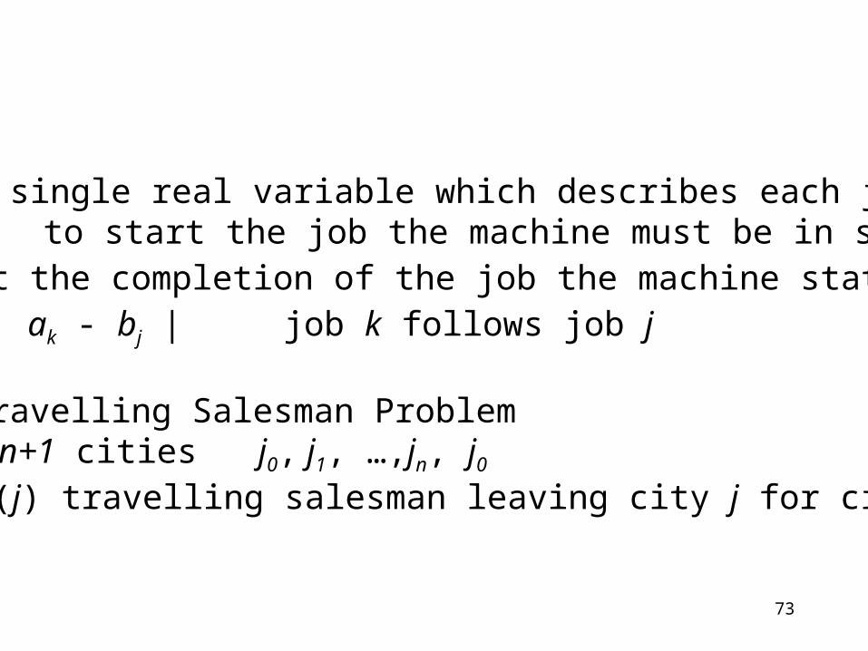
73
• a single real variable which describes each jobjob j: to start the job the machine must be in state aj ,
at the completion of the job the machine state is bj
sjk = | ak - bj | job k follows job j
• Travelling Salesman Problem with n+1 cities j0, j1, …,jn, j0
k = (j) travelling salesman leaving city j for city k

74
feasible not feasible
0 2
3 1
{0, 1, 2, 3} {2, 3, 1, 0}(0) = 2(1) = 3(2) = 1(3) = 0
0 2
3 1
{0, 1, 2, 3} {2, 1, 3, 0}
#0 #1 #2 #3
# 0
# 1
# 2
# 3
0 0 1 0
0 0 0 1
0 1 0 0
1 0 0 0job job job job
job
job
job
job
#0 #1 #2 #3
# 0
# 1
# 2
# 3
0 0 1 0
0 1 0 0
0 0 0 1
1 0 0 0job job job job
job
job
job
job

75b1
bk
bj
b2
a(1)
a(2)
a(k)
a(j)
cost of going from 1 to (1) is | a(1) - b1 |
It can be easily shown that AAAA=I, where I is the 4x4 identity matrix.Also, BBB=I, but BBBB=B≠I. So, what can you say something about testing the feasibility of permutation mapping? Also see “Hamiltonian Circuit” (Definition C.2.8. in Appendix C).
0 0 1 0
0 0 0 1
0 1 0 0
1 0 0 0
A
0 0 1 0
0 1 0 0
0 0 0 1
1 0 0 0
B
Let and

76
In some other text, the presentation of Sjk for TSP is often in a form of a matrix. Moreover, the diagonal elements of the matrix are often undefined, since the same job cannot be repeated.
#1 #2 #3
# 1
# 2
# 3
2 3
3 2
5 3job job job
job
job
job
How do we convert it to our form ?
| a2 - b1 |=2 | a3 - b1 |=3
| a1 – b2 |=3 | a3 – b2 |=2
| a1 – b3 |=5 | a2 – b3 |=3
We have 6 equations.

77
From | a2 – b1 |=2, we have a2=x+2 or x – 2.
If a2=x+2 , from | a2 – b3 |=3, we have b3=x–1 or x+5.
From | a3 – b1 |=3, we have a3=x+3 or x – 3.
If a3=x+3, from | a3 – b2 |=2, we have b2=x+1 or x+5.
From | a1 – b3 |=5, we have a1=x or x±4 or x±5 or x±10.From | a1 – b2 |=3, we have a1=x±2 or x±4 or x±8 .
Let b1=x.
If a2=x–2 , from | a2 – b3 |=3, we have b3=x–5 or x+1.
If a3=x–3, from | a3 – b2 |=2, we have b2=x–1 or x–5.
So, b3=x±1 or x±5.
So, b2=x±1 or x±5.
Choose a1=x+4, and thus, b2=x+1, b3=x–1, a2=x+2, a3=x+3.
Thus, a1=x±4.

78
To keep all entries to be positive, we can choose b1=x=2.
b1=x
b2=x+1
b3=x–1 1
2
3
a1=x+4
a2=x+2
a3=x+3
4
5
6
1 2 3
1
2
36 4 5
2
3
1
2 3
3 2
5 3a a a
b
b
b

79
Swap I(j,k) applied to a permutation produces another permutation ’:
’(k) = (j)’(j) = (k)’(l) = (l), l j , k
Consider the swap I(0,1)
0 2
3 1
{0, 1, 2, 3} {2, 1, 3, 0}
0 2
3 1
{0, 1, 2, 3} {1, 2, 3, 0}
#0 #1 #2 #3
# 0
# 1
# 2
# 3
0 0 1 0
0 1 0 0
0 0 0 1
1 0 0 0job job job job
job
job
job
job
#0 #1 #2 #3
# 0
# 1
# 2
# 3
0 1 0 0
0 0 1 0
0 0 0 1
1 0 0 0job job job job
job
job
job
job

80
5
1
7
8
910
11
6
423
1
7
8
910
11
6
423
5
Swap I(j,k) has the effect of creating two subtours out of one if j and k belongs to the same subtour.
Conversely, it combines two subtours to which j and k belong otherwise.

81
change in cost due toswap I(j, k)
bj
bk
a(j)
a(k)
abba
ababba
if)(2
if)(2||],[||
Lemma 4.5.1. If the swap causes two arrows that did nor cross earlierto cross, then the cost of the tour C I(j,k) increases and vice versa.
C I(j, k) = || [bj, bk] [a (j), a (k)] ||

82
Lemma 4.5.2. An optimal permutation mapping * is obtained ifbj ≤ bk implies a * (j) ≤ a * (k).
b1=1b2=3
b3=15
a2=4
a1=7
a3=16
If we arrange the bj in order of size and renumber the jobs so thatb1 b2 ... bn and then, optimal permutation mapping * is obtained when we arrange the a*(j) in order of size. The permutation mapping is * (j) = k where k being such that ak is the jth smallest of the a.
jobs 1 2 3 bj 1 3 15 aj 7 4 16 a*(j) 4 7 16 *(j) 2 1 3
bj 1 15 3 aj 7 16 4

83
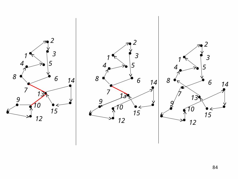
G undirected graph where arcs link the jth and (j)th nodes, j=1,…,n.
Spanning tree - a minimal set of additional arcs that connect anunconnected graph.
16
2
5
68
7
4
31
10
1211
913
15
14
16
2
5
68
7
4
31
10
1211
913
15
14
16
11
2
5
68
7
4
31
10
12
913
15
14
84
2
5
68
7
4
31
10
12
913
15
14
2
5
68
7
4
31
10
12
913
15
14
2
5
68
7
4
31
10
12
913
15
14

85
b1=1
b3=10
b2=6
a(1) =2
a(2 )=4
a(3)=11
C I(1, 2) = || [1,6] [2,4] || = 2 (4-2) = 4
C I(2, 3) = || [6,10] [4,11] || = 2 (10-6) = 8
Lower bound, sum of increase in costs of individual swaps = 4+8=12.

86
b1=1
b3=10
b2=6
a(1) =2
a(2 )=4
a(3)=11
I(1, 2) then I(2, 3)[C I(1, 2)] I(2, 3) = || [6,10] [2,11] ||
= 2 (10-6) = 8
Total increase in cost = 4+8=12.
b1=1
b3=10
b2=6
a(1) =2
a(2 )=4
a(3)=11
I(2, 3) then I(1, 2)[C I(2, 3)] I(1, 2) = || [1,6] [2,11] ||
= 2 (6-2) = 8 CHANGED!Total increase in cost =8+8=16.

87
A node is of Type 1 if bj a(j) (arrow points up)A node is of Type 2 if bj > a(j) (arrow points down)
A swap is of Type 1 if lower node is of Type 1A swap is of Type 2 if lower node is of Type 2
Swaps of Type 1 arcs can be performed starting from the top going down, so that the total increase in costs due to swaps is the same as the sum of increase of costs of individual swaps, as the overlap of intervals does not change.
Overlap of intervals unchanged Overlap of intervals changed
Individual swapsBoth Type 1 2 swaps, top first 2 swaps, bottom first

88
Swaps of Type 2 arcs can be performed starting from the bottom going up so that the total increase in costs due to swaps is the same as the sum of increase of costs of individual swaps, as the overlap of intervals does not change.
Overlap of intervals unchanged Overlap of intervals changed
Individual swapsBoth Type 2 2 swaps, bottom first 2 swaps, top first
If swaps of Type 1 are performed in decreasing order of the node indices, and swaps of Type 2 in increasing order of the node indices then there will be no change in the total increase in cost involved in the swaps as that of the sum of increase of costs of individual swaps.

89
If swaps of Type 1 are performed in decreasing order of the node indices, followed by swaps of Type 2 in increasing order of the node indices then a single tour is obtained with no change in the total increase in cost involved in the swaps as that of the sum of increase of costs of individual swaps.
Swaps of Type 1 arcs can be performed first before swaps ofType 2 arcs so that the total increase in costs due to swaps is the same as the sum of increase of costs of individual swaps.
Overlap of intervals unchanged Overlap of intervals changed
Individual swaps, Type 1 & Type 2 2 swaps, Type 1 first 2 swaps, Type 2 first
90
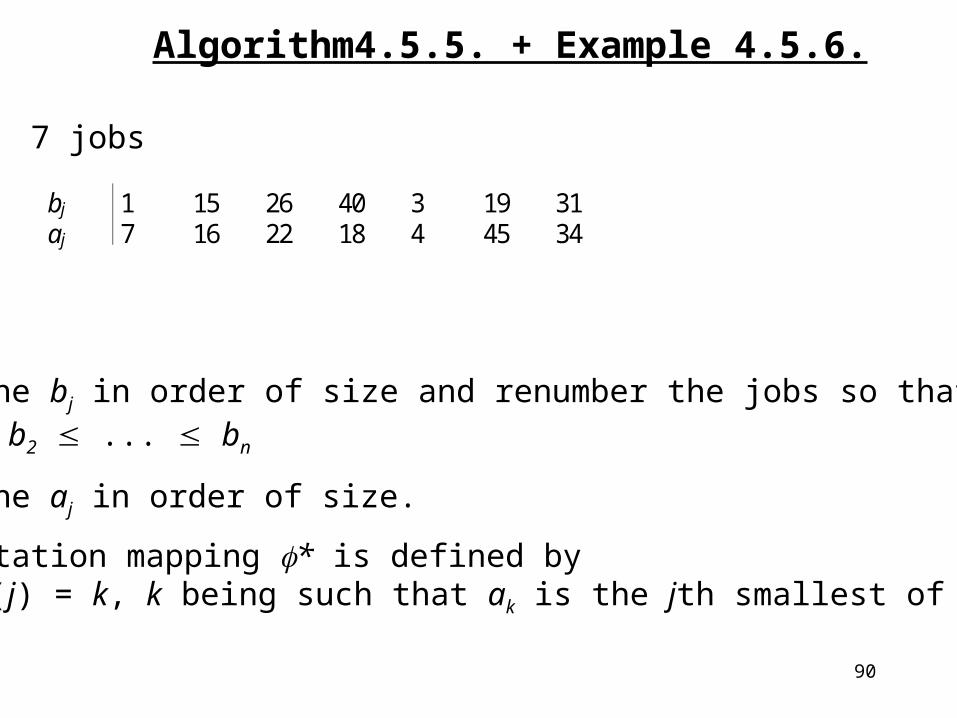
Algorithm4.5.5. + Example 4.5.6.
bj 1 15 26 40 3 19 31aj 7 16 22 18 4 45 34
Step 1. Arrange the bj in order of size and renumber the jobs so that
b1 b2 ... bn
Arrange the aj in order of size.
The permutation mapping * is defined by * (j) = k, k being such that ak is the jth smallest of the a.
7 jobs

91
jobs 1 2 3 4 5 6 7bj 1 3 15 19 26 31 40aj 7 4 16 45 22 34 18a*(j) 4 7 16 18 22 34 45*(j) 2 1 3 7 5 6 4
b4=19
b7=40
b6=31
b1=1b2=3
b3=15
b5=26
a2=4
a1=7
a3=16a7=18a5=22
a6=34
a4=45

92
Step 2. Form an undirected graph with n nodes and undirected arcs connecting the jth and *(j) nodes, j=1,…n .
If the current graph has only one component then STOP ;otherwise go to Step 3.
3
2
7
1
6
4
5

93
Step 3. Compute the swap costs C *I(j, j+1) for j=1,…,n
C* I(j, j+1) = 2 max ( min (bj+1, a*(j+1)) - max (bj, a*(j)) ), 0 )
C* I(1, 2) = 2 max ( (3-4), 0 ) = 0C* I(2, 3) = 2 max ( (15-7), 0 ) = 16C* I(3, 4) = 2 max ( (18-16), 0 ) = 4C* I(4, 5) = 2 max ( (22-19), 0 ) = 6C* I(5, 6) = 2 max ( (31-26), 0 ) = 10C* I(6, 7) = 2 max ( (40-34), 0 ) = 12

94
Step 4.Select the smallest value C* I(j, j+1) such that j is in one componentand j+1 in another. In case of a tie for smallest, choose any.
Insert the undirected arc Rj, j+1 into the graph. Repeat this step untilall the components in the undirected graph are connected.
3
2
7
1
6
4
5
4
3
2
7
1
6
4
5
4
6
3
2
7
1
6
4
5
4
6
10
3
2
7
1
6
4
5
16
4
6
10

95
Step 5.Divide the arcs added in Step 4 into two groups. Those Rj, j+1 for which bj a(j) go in group 1, those for which bj > a(j) go in group 2.
arcs bj a*(j) groupR2, 3 b2=3 a1=7 1R3, 4 b3=15 a3=16 1R4, 5 b4=19 a7=18 2R5, 6 b5=26 a5=22 2
Step 6.Find the largest index j1 such that Rj1
, j1+1 is in group 1.
Find the second largest index, and so on, up to jl assuming there arel elements in the group.
Find the smallest index k1 such that Rk1, k1+1 is in group 2.
Find the second smallest index, and so on, up to km assuming there arem elements in the group.
j1 = 3, j2 = 2, k1 = 4, k2 = 5

96
Step 7.The optimal tour ** is constructed by applying the followingsequence of swaps on the permutation *:
** = * I(j1, j1+1) I(j2, j2+1) … I(jl, jl+1) I(k1, k1+1) I(k2, k2+1) … I(km, km+1)
** = * I(3,4) I(2,3) I(4,5) I(5,6)
Type 1 Type 2
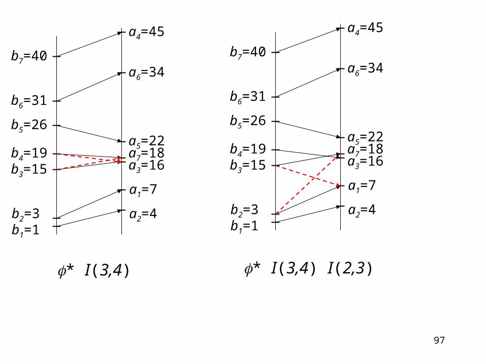
97
b4=19
b7=40
b6=31
b1=1b2=3
b3=15
b5=26
a2=4
a1=7
a3=16a7=18a5=22
a6=34
a4=45
b4=19
b7=40
b6=31
b1=1b2=3
b3=15
b5=26
a2=4
a1=7
a3=16a7=18a5=22
a6=34
a4=45
* I(3,4) * I(3,4) I(2,3)

98
b4=19
b7=40
b6=31
b1=1b2=3
b3=15
b5=26
a2=4
a1=7
a3=16a7=18a5=22
a6=34
a4=45
* I(3,4) I(2,3) I(4,5)
b4=19
b7=40
b6=31
b1=1b2=3
b3=15
b5=26
a2=4
a1=7
a3=16a7=18a5=22
a6=34
a4=45
** = * I(3,4) I(2,3) I(4,5) I(5,6)
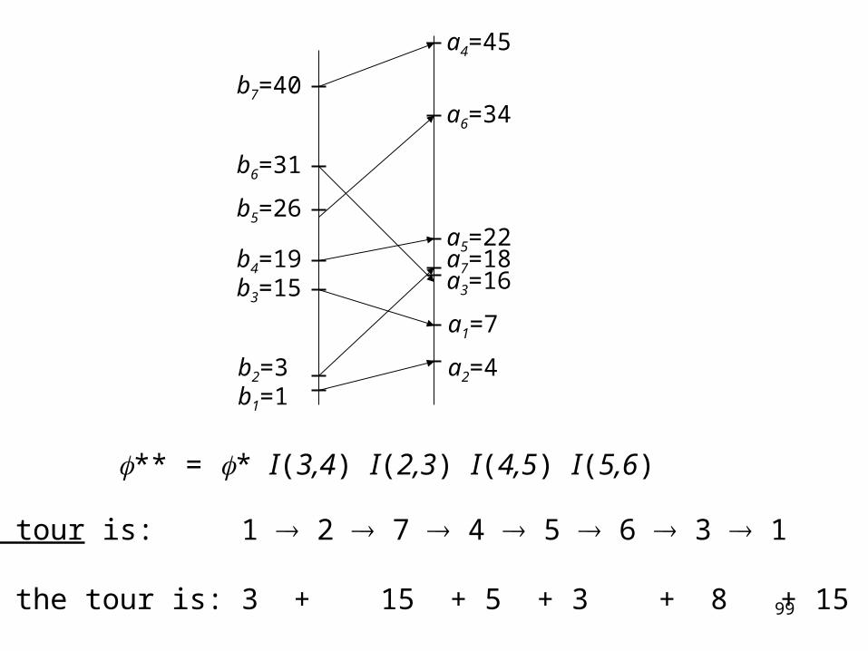
99
The optimal tour is: 1 2 7 4 5 6 3 1
The cost of the tour is: 3 + 15 + 5 + 3 + 8 + 15 + 8 = 57
** = * I(3,4) I(2,3) I(4,5) I(5,6)
b4=19
b7=40
b6=31
b1=1b2=3
b3=15
b5=26
a2=4
a1=7
a3=16a7=18a5=22
a6=34
a4=45
100
Summary
1 | Sjk | Cmax , sjk = | ak - bj | a polynomial time algorithm is given
1 | Sjk | Cmax is NP hard