98
1 Signal Transduction, Cellerator, and The Computable Plant Bruce E Shapiro, PhD [email protected] http://www.bruce-shapiro.com/cssb
| Date post: | 25-Dec-2015 |
| Category: |
Documents |
| Upload: | myra-matthews |
| View: | 218 times |
| Download: | 0 times |

1
Signal Transduction, Cellerator, and The Computable Plant
Bruce E Shapiro, PhD
[email protected]://www.bruce-shapiro.com/cssb
2
Overview
• Cellerator• Chemical Kinetics• Signal Transduction Networks
– Modular outlook– Switches, oscillators, cascades, amplifiers, etc.– Deterministic vs. Stochastic simulations
• Multicellular systems– Synchrony, pattern formation– The Computable Plant project
• Model Inference
3
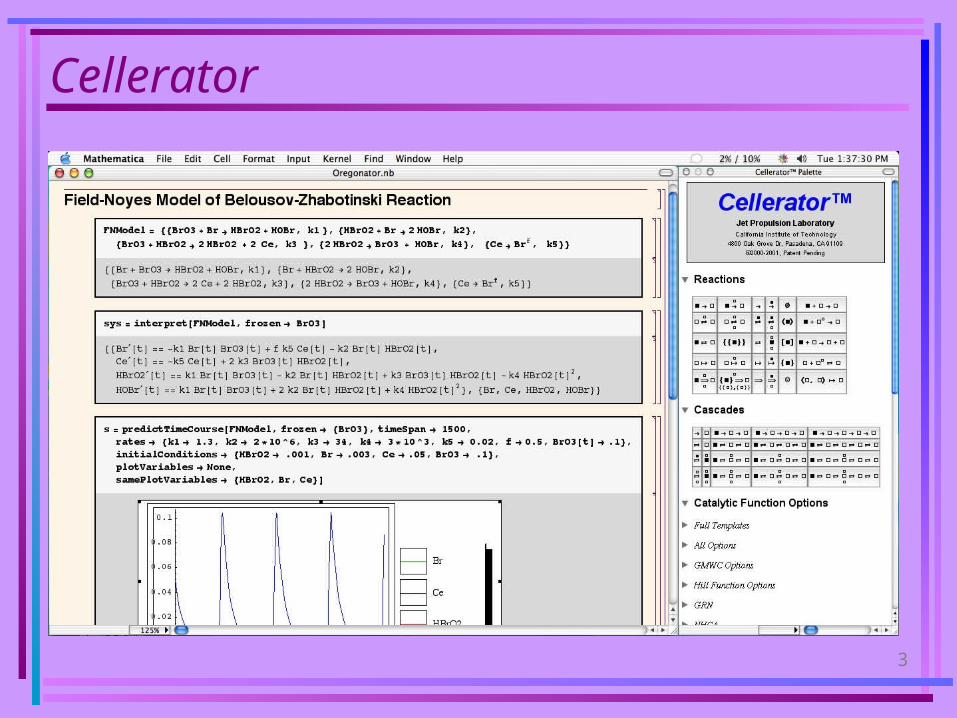
Cellerator
4
Short Cellerator Demonstration

5
• Canonical form of a chemical reaction:
• Ri,Pi: Reactants, Products• sPi,sRi: Stoichiometry• k: Rate Constant• Example:• Law of Mass Action: The rate of the reaction is proportional to
the product of the concentrations of the reactants.
•
Law of Mass Action
€
sRixii=1nR∑ k ⏐ → ⏐ sPiyii=1
nP∑
€
BrO3+ HBrO2k 3 ⏐ → ⏐ 2HBrO2+ 2Ce

6
Law of Mass Action (2)
• Formal statement (for a single reaction):
• Interpretation of
€
BrO3+ HBrO2k 3 ⏐ → ⏐ 2HBrO2+ 2Ce
€
d
dt[BrO3] = (0 −1)k3[BrO3][HBrO2] = −k3[BrO3][HBrO2]
d
dt[HBrO2] = (2 −1)k3[BrO3][HBrO2] = k3[BrO3][HBrO2]
d
dt[Ce] = (2 − 0)k3[BrO3][HBrO2] = 2k3[BrO3][HBrO2]
€
d[X]
dt= (sPX
− sRX) [Ri ]
sRi
i=1
nR
∏

7
€
BrO3+ Br k1 ⏐ → ⏐ HBrO2+ HOBr
HBrO2+ Br k 2 ⏐ → ⏐ 2HOBr
BrO3+ HBrO2k 3 ⏐ → ⏐ 2HBrO2+ 2Ce
2HBrO2k 4 ⏐ → ⏐ BrO3+ HOBr
Ce k 5 ⏐ → ⏐ Br
⎧
⎨
⎪ ⎪ ⎪
⎩
⎪ ⎪ ⎪
⎫
⎬
⎪ ⎪ ⎪
⎭
⎪ ⎪ ⎪
⇒d[HBrO2]
dt= k1[BrO3][Br] - k2[HBrO2][Br]
+ k3[BrO3][HBrO2] - k4[HBrO2]2
Law of Mass Action (3)
• Add rates for multiple reactions
“Oregonator”

8
Cellerator Input for Oregonator
stn={{BrO3+Br HBrO2+HOBr, k1}, {HBrO2+Br 2*HOBr, k2},
{BrO3+HBrO2 HBrO2+2*Ce, k3},{2*HBrO2 BrO3+HOBr, k4},
{Ce Br, k5}};interpret[stn, frozen {BrO3}];
Hold BrO3 concentration Fixed
Stoichiometry
Rate Constants

9
Cellerator Output for Oregonator
{
{Br’[t]==-k1*Br[t]*BrO3[t]+k5*Ce[t]-
k2*Br[t]*HBrO2[t], Ce’[t]==-k5*Ce[t]+2*k3*BrO3[t]*HBrO2[t], HBrO2’[t]==k1*Br[t]*BrO3[t]-
k2*Br[t]*HBrO2[t]+k3*BrO3[t]*HBrO2[t] -k4*HBrO2[t]^2,
HOBr’[t]==2*k2*Br[t]*HBrO2[t]+k4*HBrO2[t]2+k1*Br[t]*BrO3[t]},
{Br, Ce, HBrO2, HOBr}}
List of Differential Equations and Variables

10
Cellerator Simulation
s= predictTimeCourse[stn,frozen {BrO3},timeSpan 1500, rates {k1 1.3, k2 2*106, k3 34,
k4 3000., k5 0.02, BrO3[t] .1},
initialConditions {HBrO2 .001,Br .003,Ce .05,BrO3 .1};
{{0, 1500, {{Br InterpolatingFunction[{{0., 1500.}}, <>], Ce InterpolatingFunction[{{0., 1500.}}, <>], HBrO2 InterpolatingFunction[{{0., 1500.}}, <>], HOBr InterpolatingFunction[{{0., 1500.}}, <>]}}}}
Inpu
t
Out
put
11
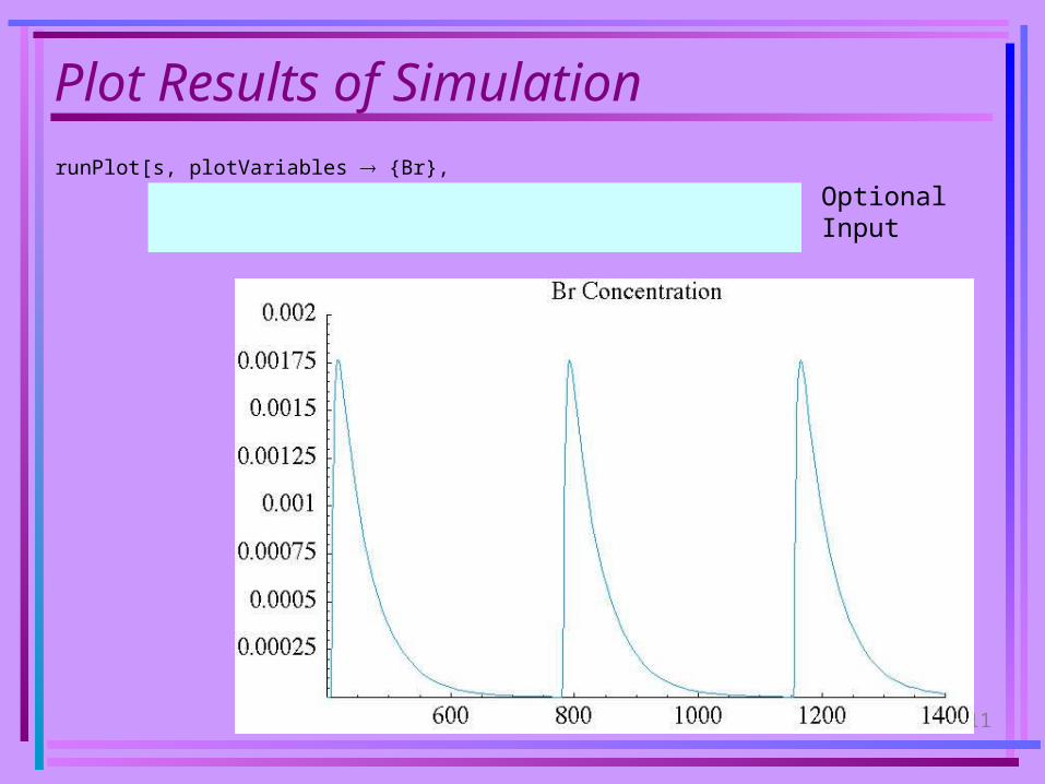
Plot Results of Simulation
runPlot[s, plotVariables {Br},PlotRange { {400, 1400}, {0, 0.002}},TextStyle {FontFamily -> Times, FontSize -> 24}, PlotLabel "Br Concentration"];
OptionalInput

12
Basic Syntax
€
network = {{reaction, rate constants},
{reaction, rate constants},...}
reaction = reactants arrow productsmodifiers
modifiers
arrow = → or ⇒ or a or E
• Format of rate constants varies for different arrows• Modifiers are optional• Different rate laws for different arrow/modifier combinations• We will focus on reaction• Generate differential equation by entering
interpret[network]

13
Basic Mass Action Reactions
€
S → P
S1 + S2 +L → P1 + P2 +L
m1S1 + m2S2 +L → n1P1 + n2P2 +L
S +L E P +L means S +L → P +L and P +L → S +L
Cellerator Syntax:
€
{S → P, k}
{S1 + S2 +L → P1 + P2 +L ,k}
{m1S1 + m2S2 +L → n1P1 + n2P2 +L , k}
{S +L E P +L ,k1,k2}
We will generally omit explicitly writing the rate constants in the remainder of this presentation.

14
Catalytic Mass Action Reactions
€
S + C → P + C becomes
€
S→C
P
€
S + CE SC → P + C or
S +C → SC
SC →S +C
SC → P +C
⎧
⎨ ⎪
⎩ ⎪
⎫
⎬ ⎪
⎭ ⎪becomes
€
SEC
P
€
S + CE SC → P + C
P + RE PR → S + R
⎧ ⎨ ⎩
⎫ ⎬ ⎭ or
S +C → SC
SC →S +C
SC → P +C
P +R → PR
PR → P +R
PR →S +R
⎧
⎨
⎪ ⎪ ⎪
⎩
⎪ ⎪ ⎪
⎫
⎬
⎪ ⎪ ⎪
⎭
⎪ ⎪ ⎪
becomes
€
SER
CP
15
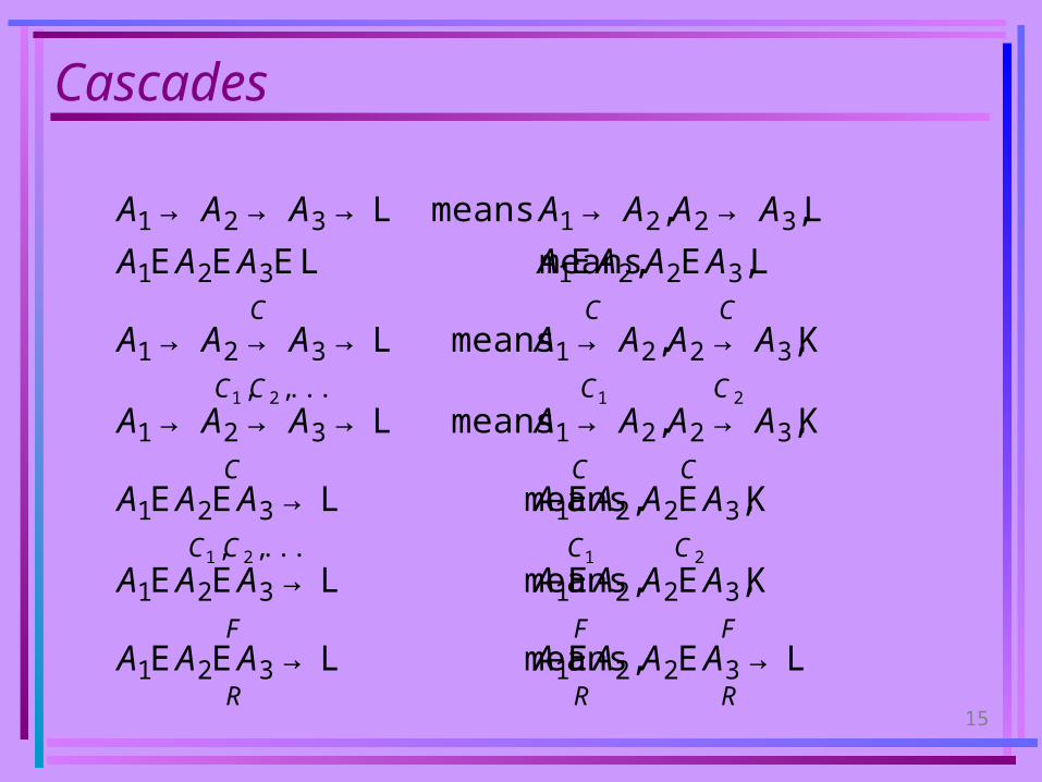
Cascades
€
A1 → A2 → A3 →L means A1 → A2, A2 → A3,L
A1E A2E A3E L means A1E A2, A2E A3,L
A1 → A2 → A3 →LC
means A1 → A2
C, A2 → A3
C,K
A1 → A2 → A3 →LC1 ,C 2 ,...
means A1 → A2
C1
, A2 → A3
C 2
,K
A1E A2E A3 →LC
means A1E A2
C, A2E A3
C,K
A1E A2E A3 →LC1 ,C 2 ,...
means A1E A2
C1
, A2E A3
C 2
,K
A1E A2E A3 →LR
F means A1E A2
R
F, A2E A3 →L
R
F
16
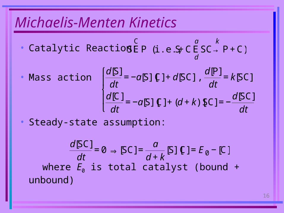
Michaelis-Menten Kinetics
• Catalytic Reaction:
• Mass action
• Steady-state assumption:
where E0 is total catalyst (bound + unbound)
€
SEC
P (i.e., S + C Ed
aSC→
kP + C)
€
d[S]
dt= −a[S][C] + d[SC],
d[P]
dt= k[SC]
d[C]
dt= −a[S][C] + (d + k)[SC] = −
d[SC]
dt
⎧
⎨ ⎪
⎩ ⎪
€
d[SC]
dt= 0⇒ [SC] =
a
d + k[S][C] = E0 −[C]

17
Michaelis-Menten Kinetics (2)
• Solve for where • Therefore
where v=kE0
• If then hence
€
[C] =E0
1+ [S]/KM
€
KM = (d + k) /a
€
d[P]
dt= k[SC] =
k[S][C]
KM=
k[S]E0
KM + [S]=
v[S]
KM + [S]
€
[SC]/ E0 <<1
€
E0 ≈ [C]
€
d[P]
dt≈
k[S][C]
KM + [S]

18
Michaelis-Menten in Cellerator
€
S ⇒ P (literally, {S ⇒ P, MM[K,v]})
means d[P]
dt=
v[S]
K + [S]= −
d[S]
dt
€
S ⇒ PC
(literally, {S ⇒ PC
, MM[K,v]})
means d[P]
dt=
v[C][S]
K + [S]= −
d[S]
dt
€
S ⇒ PC
(literally, {S ⇒ PC
, MM[a ,d, k]})
means d[P]
dt=
k[C][S]
(k + d) /a + [S]= −
d[S]
dt

19
Comparison of models
20
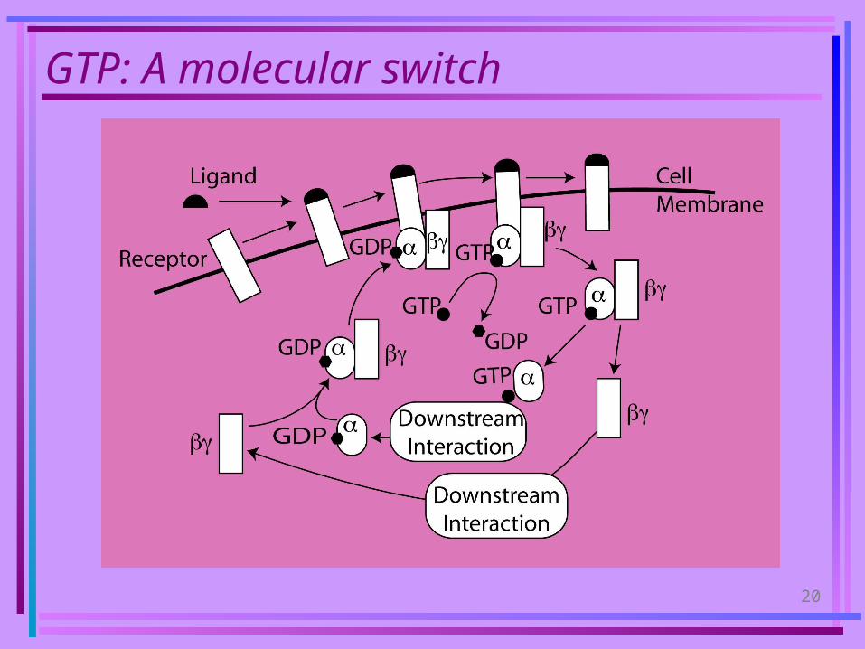
GTP: A molecular switch
21
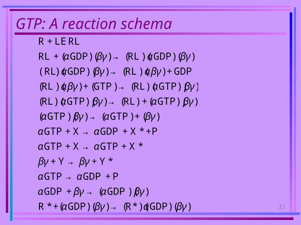
GTP: A reaction schema
€
R + LE RL
RL + (αGDP)(βγ ) → (RL)(αGDP)(βγ )
(RL)(αGDP)(βγ ) → (RL)(αβγ ) + GDP
(RL)(αβγ ) + (GTP) → (RL)(αGTP)(βγ )
(RL)(αGTP)(βγ ) → (RL) +(αGTP)(βγ )
(αGTP)(βγ ) → (αGTP) + (βγ )
αGTP + X → αGDP + X * +P
αGTP + X → αGTP + X *
βγ + Y → βγ + Y*
αGTP → αGDP + P
αGDP + βγ → (αGDP)(βγ )
R *+(αGDP)(βγ ) → (R*)(αGDP)(βγ )

22
GTP: Cellerator schema

23
GTP: Cellerator Simulation

24
RASGTP Switch

25
Cascades

26
MAPK: Mitogen Activate Protein Kinase
Cell Growth and Survival
Heat Shock, Radiation, Chemical, Inflamatory
Stress
lab of Jim Woodget, http://kinase.uhnres.utoronto.ca/

27
MAPK Cascade
€
KE K∗E K∗∗
Ph3
KK∗∗
€
KKE KK∗E KK∗∗
Ph2
KKK∗
€
KKKE KKK∗
Ph1
S
Reactions in solution (no scaffold)

28
MAPK in Solution Kinase Reactions
1st Stage
KKK+SKKK-SKKK-S KKK+SKKK-SKKK*+S
2nd Stage (1st Phosphate group)
KK+KKK*KK-KKK*
KK-KKK*KK+KKK*
KK-KKK*KKK*+KK*
2nd Stage (2nd Phosphate group)
KKK*+KK*KK*-KKK*
KK*-KKK*KKK*+KK*
KK*-KKK*KKK*+KK**
3rd Stage (1st Phosphate group)
K+KK**K-KK**
K-KK**K+KK**
K-KK**KK**+K*
3rd Stage (2nd Phosphate group)
KK**+K*K*-KK**
K*-KK**KK**+K*
K*-KK**KK**+K**
Phosphatase Reactions
1st Stage
KKK*+Ph1KKK*-Ph1
KKK*-Ph1 KKK+ Ph1
KKK*- Ph1 KKK*+ Ph1
2nd Stage (1st Phosphate group)
KK*+Ph2KK*-Ph2
KK*- Ph2 KK+ Ph2
KK*- Ph2 KK*+ Ph2
2nd Stage (2nd Phosphate group)
KK**+Ph2KK**-Ph2
KK**- Ph2 KK*+ Ph2
KK**- Ph2 KK**+ Ph2
3rd Stage (1st Phosphate group)
K*+Ph3K*-Ph3
K*- Ph3 K+ Ph3
K*- Ph3 K*+ Ph3
3rd Stage (2nd Phosphate group)
K**+Ph3K**-Ph3
K**- Ph3 K*+ Ph3
K**- Ph3 K**+ Ph3

29
MAPK Cascade on Scaffold
• Scaffold binding significantly increases the rate of phosphorylation
• Scaffold has 3 slots: one for each kinase• Each slot can be in different states
– Slot 1: empty, KKK, or KKK* bound– Slot 2: empty, KK, KK*, or KK** bound– Slot 3: empty, K, K*, K** bound
• Enter/leave scaffold in any order• KKK* and either KK or KK* must be bound at same
time produce KK**, etc.• Number of reactions increases exponentially with
number of slots

30
Effect of Scaffold on SimulationsNumber of Reactions
10
100
1000
10000
100000
2 3 4 5 6
Number of slots (N)
Single Phosphorylation
Double Phosphorylation

31
Reactions in MAP Kinase Cascade
• Phosphorylation in Solution
• Binding to Scaffold
• Phosphorylation in Scaffold
Kij ⇔
Phi
Ki+1ai+1
Kij+1 i =1,K ,n−1, j =0,K ,aj −1
⎧ ⎨ ⎪
⎩ ⎪
⎫ ⎬ ⎪
⎭ ⎪
Sp1,L ,pi=ε,L ,pn +Ki
j ↔ Sp1,L ,pi=j,L ,pn{ }, pi =ε,0,1,K ,ai, i ≠ j
0,1,K ,ai, i = j
⎧ ⎨ ⎩
Sp1,L ,pi−1=j<ai−1,pi=ai ,L ,pn+K ⇔ Sp1,L ,pi−1=j+1,pi=ai,L ,pn{ }
Sp1,L ,pi−1=j<ai−1,pi=ai ,L ,pn → Sp1,L ,pi−1=j+1,pi=ai ,L ,pn{ }

32
Effect of Scaffold on MAPK00.10.20.30.40.50.60.70.800.511.52 Scaffold ConcentrationControl*K4 - K3 complex formationPhosphatases in scaffoldEqual rate constants*** Control Simulation: k2/k1=1000, no phosphatases, K4 does not form complex
** k2/k1=1 (rate constants for phosphorylation steps of MAPK and MAPKKK)MAPK**0100∫dt
33
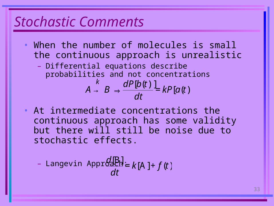
Stochastic Comments
• When the number of molecules is small the continuous approach is unrealistic– Differential equations describe probabilities and not
concentrations
• At intermediate concentrations the continuous approach has some validity but there will still be noise due to stochastic effects.
– Langevin Approach:
€
A → Bk
⇒dP[b(t)]
dt= kP[a(t)]
€
d[B]dt
= k[A]+ f (t)

34
Direct Stochastic Algorithm
Gillespie Algorithm (1/3):• At any given time, determine which reaction is
going to occur next, and modify numbers of molecules accordingly
€
Reactions : R1,R2,...,RN
Rate Constants : k1,k2,...,kn
Concentrations : X1,X2,..., XM in volume V
Numbers : Ni = XiV
State of system at t : {X1,X2,...,XM }
# of Distinct Molecular Combinations in Ri : h1,h2,...,hN
hi depends combinatorically on the X1,X2,...,XM Gillespie DT (1977) J. Phys. Chem. 81: 2340-2361.
35
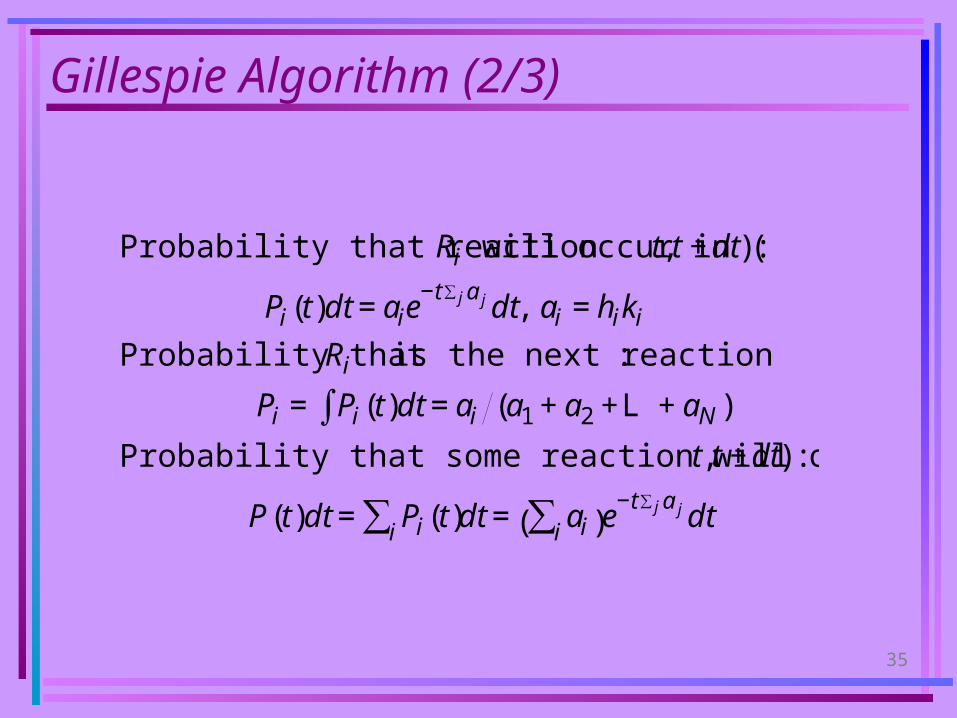
Gillespie Algorithm (2/3)
€
Probability that reaction Ri will occur in (t, t + dt) :
Pi (t)dt = aie−t a jj∑
dt, ai = hiki
Probability that Ri is the next reaction :
Pi = Pi (t)dt∫ = ai (a1 + a2 +L + aN )
Probability that some reaction will occur in (t, t + dt) :
P(t)dt = Pi (t)i∑ dt = aii∑( )e−t a jj∑
dt

36
Gillespie Algorithm (3/3)
Let t=0
While t<tmax {
Calculate all the ai=hiki and a0=aj
Generate two random numbers r1, r2 on (0, 1)
The time until the next reaction is =(1/a0)ln(1/r1)Set t = t + Reaction Rj occurs at t, where j satisfies
a1+a2+…+aj-1 < r2a0 ≤ aj+aj+1+…+an
Update the X1,X2,…,Xn to reflect the occurance of reaction Rj
}
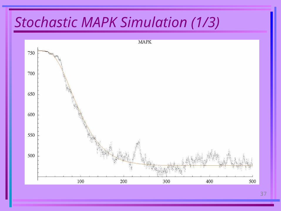
37
Stochastic MAPK Simulation (1/3)

38
Stochastic MAPK Simulation (2/3)
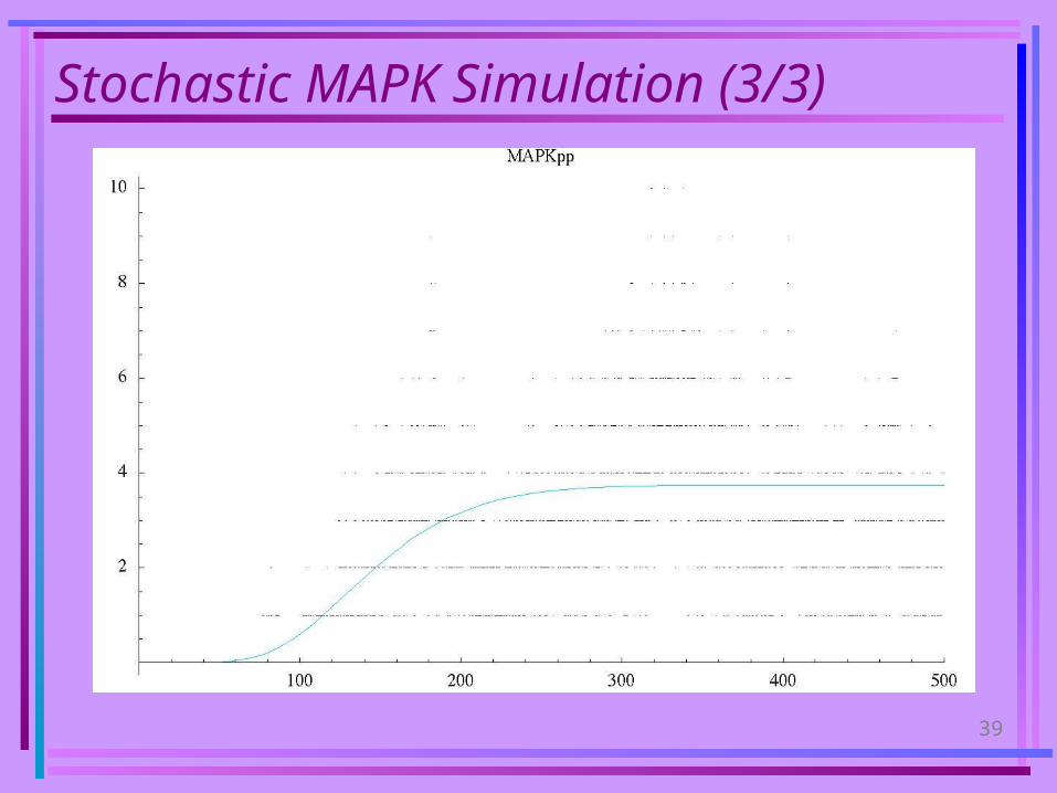
39
Stochastic MAPK Simulation (3/3)

40
Analysis of Multi-step reactions
€
X + nL Ed
aZ
€
d[Z ]dt
= a[X][L]n − d[Z ] = 0
[X]SS =d[Z ]SS
a[L]n = N −[Z ]SS
N =[X]+[Z ]
[Z ]SS =N[L]n
[L]n +(d /a)
Steady State Solution
Adding steps increases sensitivity
€
X + L Ed
aXL, XL + L E
d
aXLL, XLL + L E
d
aXLLL, L XLn−1 + L E
d
aXLn
Simplify to:

41
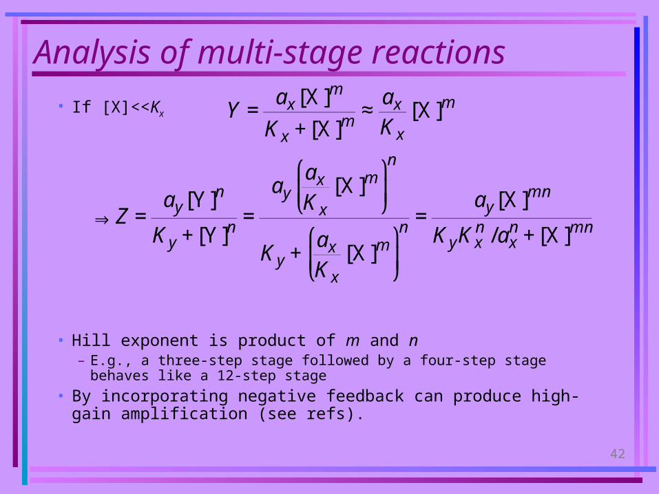
Analysis of multi-stage reactions
• Consider two stages of a cascade with m and n steps
• Steady State:
€
Y =ax[X]m
Kx +[X]m , Z =ay[Y]n
Ky +[Y]n
€
Z =
ayax[X]m
Kx +[X]m
⎡
⎣ ⎢
⎤
⎦ ⎥
n
Ky +ax[X]m
Kx +[X]m
⎡
⎣ ⎢
⎤
⎦ ⎥
n =ayax
n[X]mn
Ky Kx +[X]m( )
n+ ax
n[X]mn
42
Analysis of multi-stage reactions
• If [X]<<Kx
• Hill exponent is product of m and n– E.g., a three-step stage followed by a four-step stage behaves like a
12-step stage
• By incorporating negative feedback can produce high-gain amplification (see refs).
€
Y =ax[X]m
Kx +[X]m ≈ax
Kx[X]m
⇒ Z =ay[Y]n
Ky +[Y]n =
ayax
Kx[X]m ⎛
⎝ ⎜
⎞
⎠ ⎟n
Ky +ax
Kx[X]m ⎛
⎝ ⎜
⎞
⎠ ⎟n =
ay[X]mn
KyKxn /ax
n +[X]mn

43
Oscillators in Nature
• Where they occur (to name a few):– Circadian rhythms– Mitotic oscillations– Calcium oscillations– Glycolysis– cAMP– Hormone levels
• How they occur: feedback– Both negative & positive feedback systems– Some have feed-forward loops also

44
Negative feedback: canonical model*
€
dxdt
= S −αx − βy, dydt
= γx −δy, α ,β ,γ ,δ ≥ 0
€
′ ′ x − 2a ′ x +bx =δS, a = −(α +δ) /2 ≤ 0, b =αδ + βγ ≥ 0
Equivalent second order system:0
Characteristic equation:
€
r2 − 2ar +b = 0⇒ r = a ± a2 −b
€
a2 < b⇒ stable spiral
a = 0⇒ undamped oscillations
δS /b = steady state
QuickTime™ and aTIFF (LZW) decompressor
are needed to see this picture.
*Hoffmann et al (2002) Science 298:1241a=0.25,b=10,=1,S=5

45
2-species ring oscillator
X X*
Y
Y*
€
X ⇒ X*Y
,Y ⇒ Y *X*
, X* ⇒ XY *
,Y * ⇒ YX
€
d[X]dt
=v3(1−[X])(1−[Y])
1+ KM 3 −[X]−
v1[X][Y]KM1 +[X]
d[Y]dt
=v4[X](1−[Y])1+ KM 4 −[Y]
−v2 (1−[X])[Y]
KM 2 +[Y]
€
X + X* =1
Y +Y * =1

46
3-species ring oscillator
X X*
Y Y*
Z Z*
€
X ⇒ X*Z
,Y ⇒ Y *X
,Z ⇒ Z*Y
, X* ⇒ XZ*
,Y * ⇒ YX*
, Z* ⇒ ZY *
€
d[X]dt
=v(1−[X])(1−[Z])
1+ KM −[X]−
v[X][Z]KM +[X]
d[Y]dt
=v(1−[X])(1−[Y])
1+ KM −[Y]−
v[X][Y]KM +[Y]
d[Z]dt
=v(1−[Y])(1−[Z])
1+ KM −[Z]−
v[Y][Z]KM +[Z]

47
3-species Ring Oscillator
v=10KM
Robust oscillations
v=KM
Damped oscillations

48
Repressilator
Z PZ
Y PY
X PX
φ
φφφ
φφ
RNA
RNA
RNA
Constructed in E. coliElowitz & Leibler, Nature 403:335 (2000)

49
Repressilator Model Simulations
€
d[X]dt
=α 0 +α +α1[PY]n
K n +[PY]n − k[X], d[PX]
dt= β{[X]−[PX]}
d[Y]dt
=α 0 +α +α1[PZ]n
K n +[PZ]n − k[Y], d[PY]
dt= β{[Y]−[PY]}
d[Z ]dt
=α 0 +α +α1[PX]n
K n +[PX]n − k[Z], d[PZ]
dt= β{[Z]−[PZ]}

50
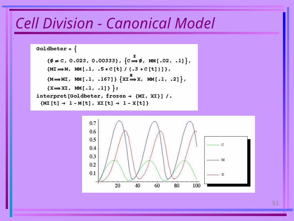
Cell Division - Canonical Model
MI M
XI X
C φφ
Goldbeter (1991) PNAS USA, 88:9107
€
d[C]dt
= 0.023− 0.00333[C]−0.1[C][X]0.02 +[C]
d[M]dt
=0.5[C](1−[M])
(0.3+[C])(1.1−[M])−
0.167[M]0.1+[M]
d[X]dt
=0.1[M](1−[X])
1.1−[X]−
0.1[X]0.1+[X]
“Minimal” Model of Cell Division
51
Cell Division - Canonical Model

52
Multi-cellular networks
€
ddt
xij = f (x1
j ,..., xNj )+ Λjkg jk (x1
k ,..., xNk )
k∈Nbr( j)∑
+ M ijk (xik − xk
j )k∈Nbr( j)∑
Intracellular Networke.g., of mass action, etc.
Transport, ligand/receptor interactions, etc
Diffusion Tensor
Connection matrixSet of neighbors
of cell j
Species xi in cell j

53
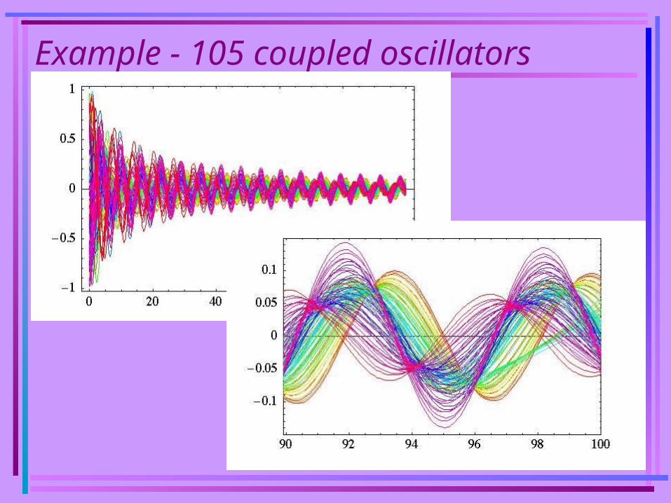
Example - coupled oscillators
€
n Coupled Oscillators
′ ′ x i +ω2xi + α jx jj∈nbr(i)∑ = 0
i =1,2,...,n
€
Two Coupled Oscillators
′ ′ x +ω2x +αy = 0
′ ′ y +ω2y +αx = 0
Two uncoupled Oscillators Two Coupled Oscillators, =.1
54
Example - 105 coupled oscillators

55
Example - 105 coupled oscillators
QuickTime™ and aVideo decompressor
are needed to see this picture.

56
Coupled nonlinear oscillators
MI M
XI X
C φφ
MI M
XI X
C φφ
MI M
XI X
C φφ
MI M
XI X
C φφ
MI M
XI X
C φφ
MI M
XI X
C φφ
Arbitrarily let species X in CMX model diffuse to adjacent cells

57
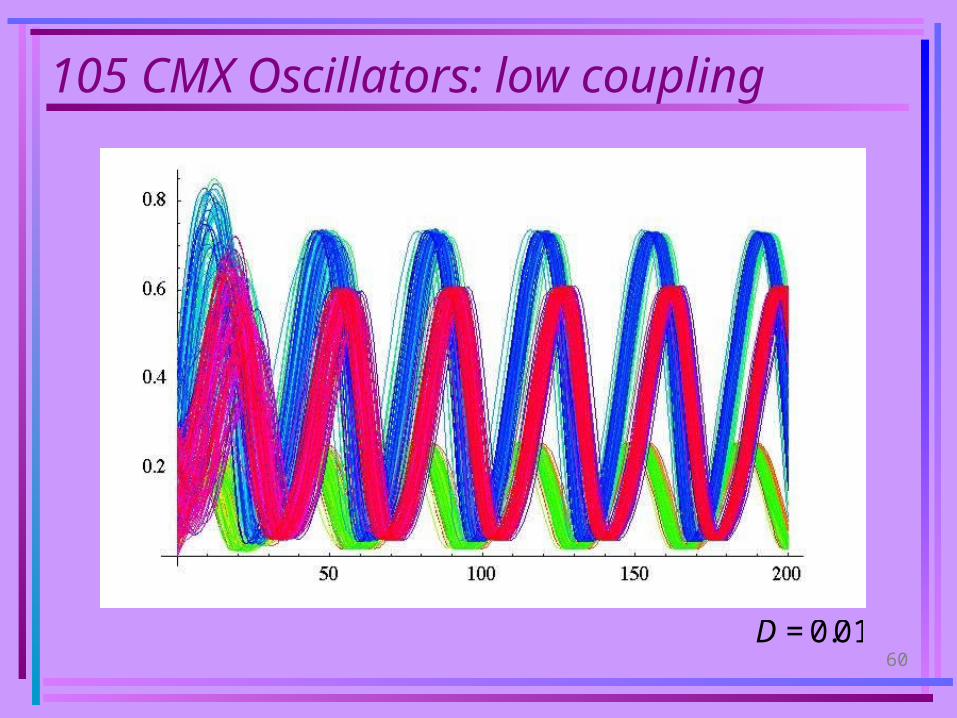
Coupled CMX Oscillators
€
d[C j]
dt= 0.023− 0.00333[C j]−
0.1[C j][X j]
0.02 +[C j]
d[M j]
dt=
0.5[C j](1−[M j])
(0.3+[C j])(1.1−[M j])−
0.167[M j]
0.1+[M j]
d[X j]
dt=
0.1[M j](1−[X j])
1.1−[X j]−
0.1[X j]
0.1+[X j]+ D ([Xk ]−[X j])k∈Nbrs( j)∑
•All oscillating at same frequency•But different phases•What happens if you have 105 coupled oscillators with random phase shifts?

58
105 CMX Oscillators: uncoupled

59
105 CMX Oscillators: uncoupled
QuickTime™ and aVideo decompressor
are needed to see this picture.
60
105 CMX Oscillators: low coupling
€
D = 0.01

61
105 CMX Oscillators: higher coupling
€
D = 0.1

62
105 CMX Oscillators: higher coupling
€
D = 0.1
QuickTime™ and aVideo decompressor
are needed to see this picture.

63
105 CMX Oscillators: Random Period
Uncoupled motion

64
105 CMX Oscillators: Random Period
€
D = 0.1

65
105 CMX Oscillators: Random Period
QuickTime™ and aAnimation decompressor
are needed to see this picture.
QuickTime™ and aAnimation decompressor
are needed to see this picture.
Uncoupled Coupled Oscillators

66
Pattern Formation
Activator-Inhibitor Models
Single Diffusing Species
•Self-activating (locally)
•Self-inhibitory (externally)
Two Diffusing Species
•X: Activator
•Y: Inhibitor
A φ
A φ
A φ
X Y φφ
X Y φφ

67
Two species pattern formation model
Continuous model*:
€
d[X]dt
= a −b[X]−[X]2 /[Y]+ D1∇2[X]
d[Y]dt
=[X]2 −[Y]+ D2∇2[Y]
Discrete implementation:
€
{∅E X j , a, b}, {Y j →∅ , 1},
{X j → X j +Y j , X j}, {2X j → X j , 1/Y j},
{X jE Xi , D1}, {Y jE Yi , D2}
*See Murray Chapter 14 for detailed analysis

68
Single species pattern formation model
Continuous (logistic) model:
€
d
dt[A] = v[A](1−[A]/K) −
vM [A] [Anbr ]nbrs∑
[A] + KM
Discrete implementation:
€
A[i] Ev /K
v2A[i], rate constants v, v/K
A[ j]⇒ ∅A[ i ]
, Michaelis constants vM ,KM
Steady State Equation (v=K=vM=KM=1, x=[A])
€
0 = x(1− x) −x
1+ xxii∑ ⇒ x = 0 or 0 =1− x2 − xii∑
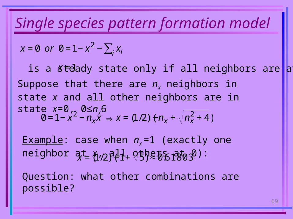
69
Single species pattern formation model
€
x = 0 or 0 =1− x2 − xii∑
€
x =1 is a steady state only if all neighbors are at x=0
Suppose that there are nx neighbors in state x and all other neighbors are in state x=0, 0≤nx6
€
0 =1− x2 − nx x ⇒ x = (1/2)(−nx + nx2 + 4)
Example: case when nx =1 (exactly one neighbor at x, all others at 0):
Question: what other combinations are possible?
€
x = (1/2)(−1+ 5) ≈ 0.618034
70
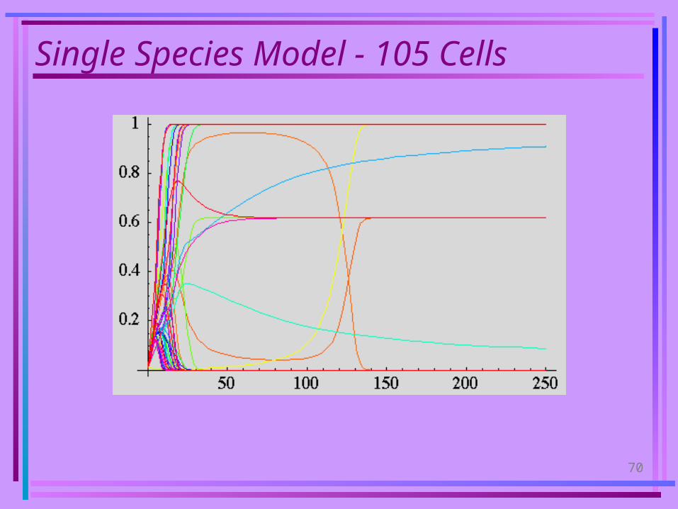
Single Species Model - 105 Cells

71
Single Species Model - 105 Cells
QuickTime™ and aVideo decompressor
are needed to see this picture.
72
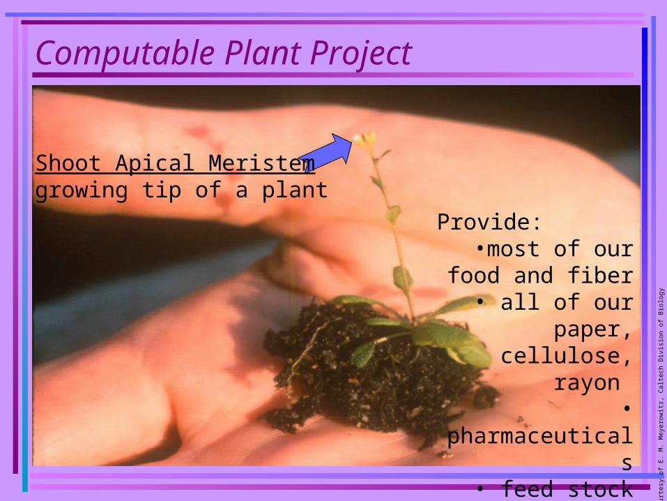
Provide:•most of our food and
fiber• all of our paper, cellulose, rayon
• pharmaceuticals• feed stock
• waxes• perfumes
Shoot Apical Meristemgrowing tip of a plant
Imag
e co
urte
sy o
f E
. M. M
eyer
owitz
, Cal
tech
Div
isio
n of
Bio
logy
Computable Plant Project

73
Computable Plant Project
• NSF (USA) Frontiers in Integrative Biological Research (FIBR) Program
• S/W Architecture: Production-scale model inference– Models formulated as cellerator reactions or SBML– C++ simulation code autogenerated from models– Mathematical framework combining transcriptional regulation,
signal transduction, and dynamical mechanical models– Simulation engine including standard numerical solvers and
plot capability– Nonlinear optimization and parameter estimation– ad hoc image processing and data mining tools
• Image Acquisition– Dedicated Zeiss LSM 510 meta upright laser scanning
confocal microscope.• http://www.computableplant.org

74
Computable Plant Project
ExperimentsData Mining
Data Sets
AutomatedCode Generation
Optimization
Simulation
Mathematical ModelGeneration
Regulations &Reactions
Online
Solvers Plotters
Local
User

75
Model Organism
Arabidopsis Thaliana
76
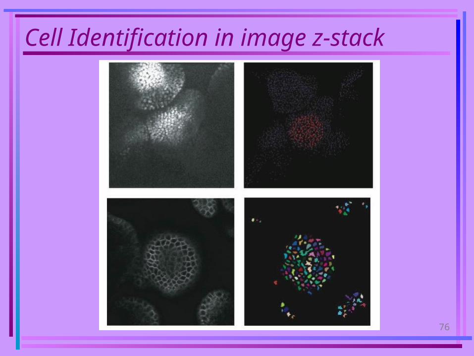
Cell Identification in image z-stack
77
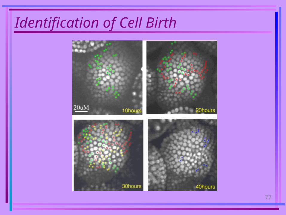
Identification of Cell Birth

78
Imag
e co
urte
sy o
f E
. M. M
eyer
owitz
, Cal
tech
Div
isio
n of
Bio
logy
Shoot Apical Meristem

79
Meristem Pattern Maintenance Model
80
Simulation of Meristem Growth
QuickTime™ and aVideo decompressor
are needed to see this picture.

81
Systems Biology Markup Language
http://sbml.org
libsbml (C++)
MathSBML (Mathematica)
82
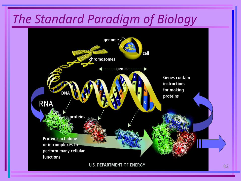
The Standard Paradigm of Biology
RNA

83
Microarrays Produce a lot of data!
Affymetrix GeneChip® microarray. Images courtesy of Affymetrix.
84
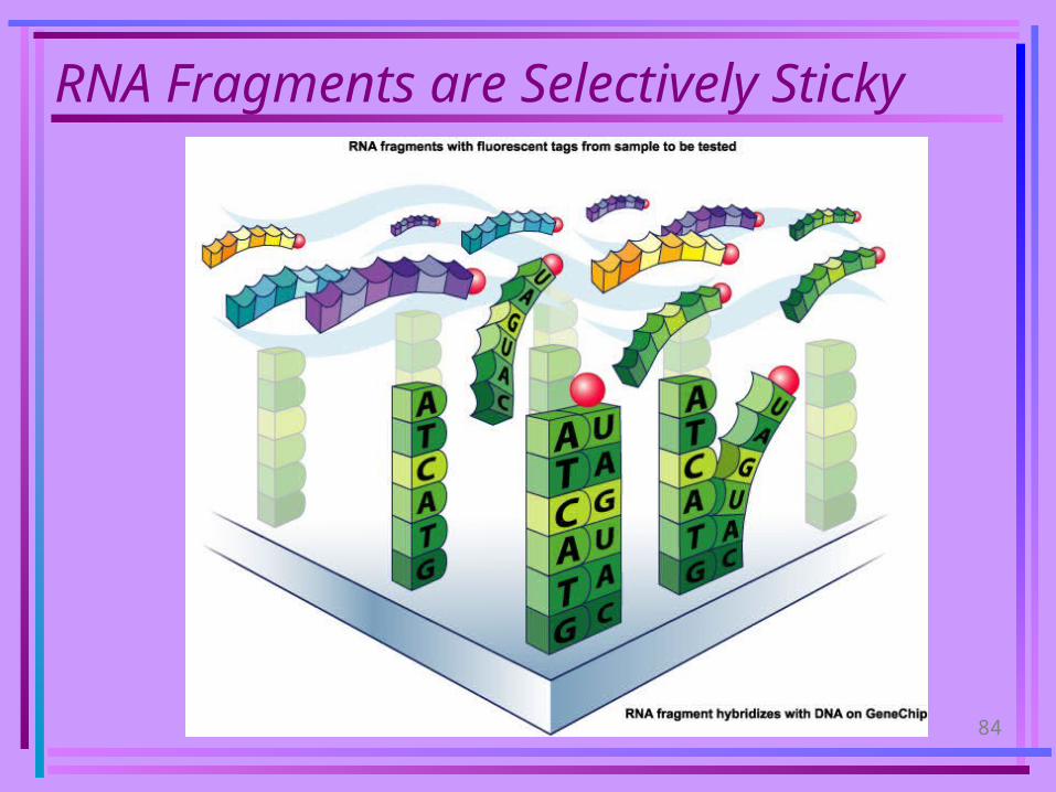
RNA Fragments are Selectively Sticky
85
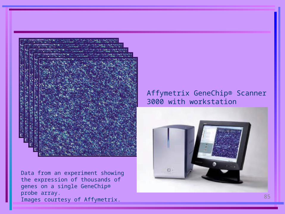
Affymetrix GeneChip® Scanner 3000 with workstation
Data from an experiment showing the expression of thousands of genes on a single GeneChip® probe array. Images courtesy of Affymetrix.

86
Model Inference: Fitting A Model to Data
• Cluster to reduce data size
• Use simplest possible mathematical possible to determine connectivity– Fit parameters with some optimization
process: simulated annealing, least squares, steepest descent, etc.
– Refine model with biological knowledge– Refine with better accurate math model– … and repeat until done …

87
Clustering
Time
Ge
ne

88
Data clusters in two dimensions
x
y
Concentration at time t1
Con
cent
rati
on a
t ti
me
t 2
Plot ([X[t3 1],X[t2],X[t3],…,X[tn]) for every species
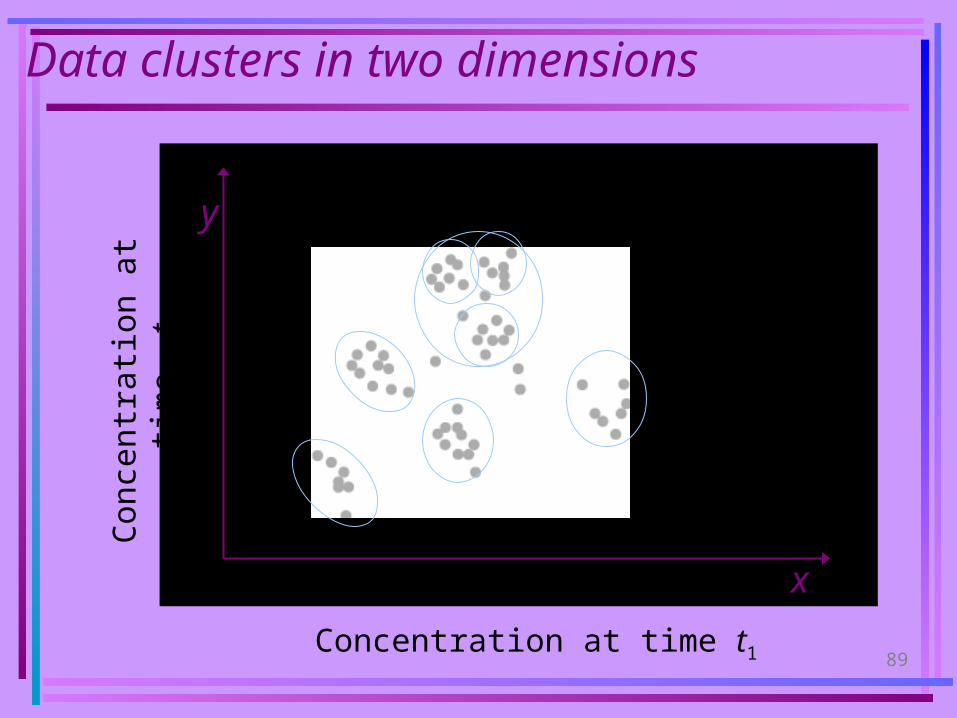
89
Data clusters in two dimensions
x
y
Concentration at time t1
Con
cent
rati
on a
t ti
me
t 2
90
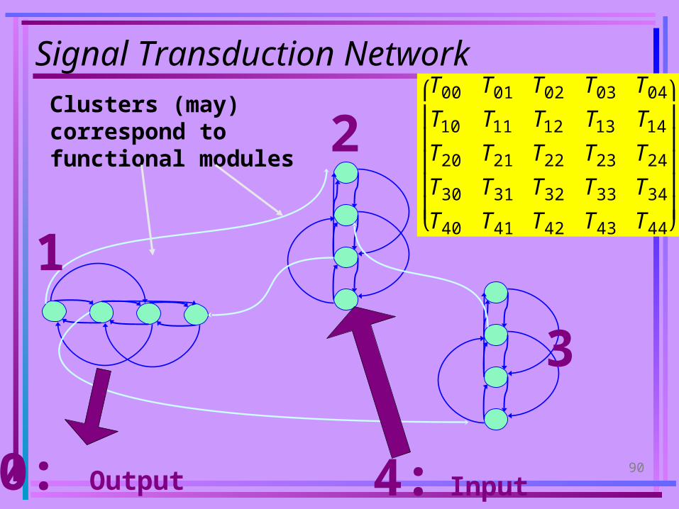
Clusters (may) correspond to functional modules
4: Input0: Output
Signal Transduction Network
1
2
3€
T00 T01 T02 T03 T04
T10 T11 T12 T13 T14
T20 T21 T22 T23 T24
T30 T31 T32 T33 T34
T40 T41 T42 T43 T44
⎛
⎝
⎜ ⎜ ⎜ ⎜ ⎜
⎞
⎠
⎟ ⎟ ⎟ ⎟ ⎟
91
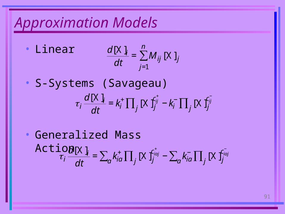
Approximation Models
• Linear
• S-Systems (Savageau)
• Generalized Mass Action
€
d[X]idt
= M ij[X] jj=1
n
∑
€
id[X]i
dt= kia
+ [X] jciaj
+
j∏a∑ − kia− [X] j
ciaj−
j∏a∑€
id[X]i
dt= ki
+ [X] jcij
+
j∏ − ki− [X] j
cij−
j∏

92
Approximation Models
• Generalized Continuous Sigma-Pi Networks
€
id[X]i
dt= g(ui + h j )
ui = ˆ M ijk [X] j[X]kk∑j∑ + M jk [X] jj∑
g(x) =12
1+x
1+ x2
⎛
⎝ ⎜
⎞
⎠ ⎟
93
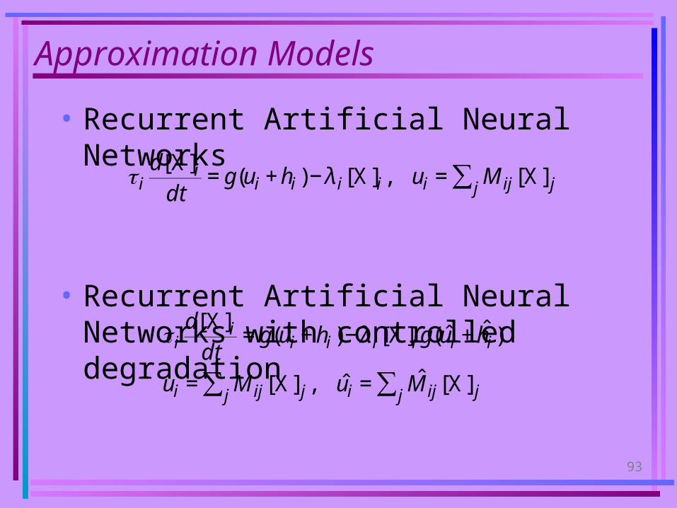
Approximation Models
• Recurrent Artificial Neural Networks
• Recurrent Artificial Neural Networks with controlled degradation€
id[X]i
dt= g(ui + hi ) − λ i[X]i , ui = M ij[X] jj∑
€
id[X]i
dt= g(ui + hi ) − λ i[X]i g( ˆ u i + ˆ h i )
ui = M ij[X] jj∑ , ˆ u i = ˆ M ij[X] jj∑

94
Approximation Models
• Recurrent Artificial Neural Networks with biochemical knowledge about some species
€
id[X]i
dt= g(ui + hi ) − λ i[X]i + τ i
d[X]idt Cellerator
ui = M ij[X] jj∑
Known or hypothesized interactions due to mass action, Michaelis-Menten, or other reactions (A priori knowledge or assumptions)

95
Approximation Models
• Multicellular Artificial Neural Networks with biochemical knowledge about some species:
€
ad[X]a
i
dt= g(ua
i + ha ) − λ a[X]ai +γa[X]a
i +δa[X]a,exti
+τ id[X]i
dt Cellerator
€
uai = Mab[X]b
ib∑
+ Λijj∑ ˆ M ab[X]b
jb∑ + [X]c
i ˜ M ac(1) ˜ M cb
(2)[X]bj
b∑c∑( )
Resources
Diffusion
Lower index: species; Upper Index: CellGeometric
Connections
96
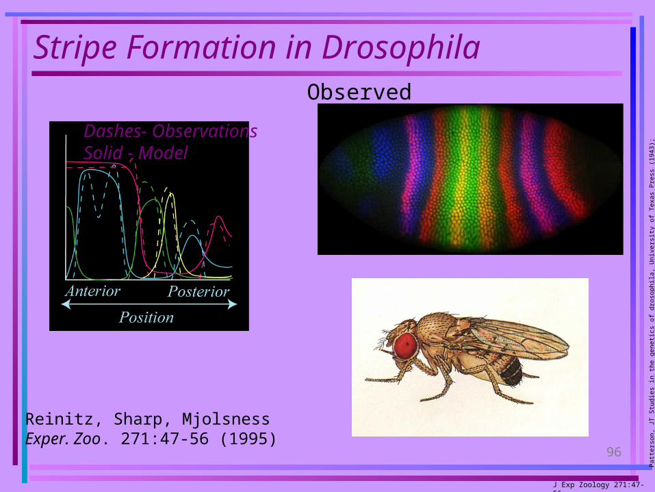
Stripe Formation in Drosophila
J Exp Zoology 271:47-56
Dashes- ObservationsSolid - Model
Patte
rson
, JT
Stu
dies
in th
e ge
netic
s of
dro
soph
ila, U
nive
rsity
of
Tex
as P
ress
(19
43);
http
://fl
ybas
e.bi
o.in
dian
a.ed
u:82
/ana
tom
y/D
roso
philaObserved
Reinitz, Sharp, MjolsnessExper. Zoo. 271:47-56 (1995)
97
Some Important Meetings
• ISMB-2004, Scotland, ≈ 30 July 04Intelligent Systems in Molecular Biology
2003: Australia; 2005: US; 2006:Brazil
• ICSB-2004, Heidelberg, Oct 04International Conference on Systems Biology
SBML Forum held as satellite meeting
2003:US; 2002:Sweden; 2001:US; 2000: Japan
• PSB-2005, Hawaii, Jan 05 Pacific Symposium on Biocomputing
• RECOMB, Spring 05 Research in Computational Molecular Biology
• BGRS-04, July 04, Semiannually in NovosibirskBioinformatics of Genome Regulation and Structure
• Satellite meetings of many major biology and computer science meetings: SIAM, ACB, IEEE, ASCB (US), Neuroscience, IBRO,..

98
Collaborators
• CelleratorCellerator– Eric Mjolsness, U. California, Irvine (Computer )Eric Mjolsness, U. California, Irvine (Computer )
– Andre Levchenko, Johns Hopkins (Bioengineering)Andre Levchenko, Johns Hopkins (Bioengineering)
• Computable Plant - Eric Mjolsness, PIComputable Plant - Eric Mjolsness, PI– Elliot Meyerowitz, Caltech (Biology)Elliot Meyerowitz, Caltech (Biology)
– Venu Reddy, Caltech (Biology)Venu Reddy, Caltech (Biology)
– Marcus Heisler, Caltech (Biology)Marcus Heisler, Caltech (Biology)
– Henrik Jonsson, Lund, Sweden (Physics)Henrik Jonsson, Lund, Sweden (Physics)
– Victoria Gor, JPL (Machine Learning)Victoria Gor, JPL (Machine Learning)
• SBML (John Doyle, PI, Caltech; H. Kitano, Japan)SBML (John Doyle, PI, Caltech; H. Kitano, Japan)
– Mike Hucka, Caltech (Control & Dynamical Systems)Mike Hucka, Caltech (Control & Dynamical Systems)
– Andrew Finney, University of Hertfordshire, UKAndrew Finney, University of Hertfordshire, UK


