Page 1
1 Stationary Process
Model: Time invariant mean
yt = �+ "t
1.1 De�nition:
1. Autocovariance
jt = E (yt � �) (yt�j � �) = E ("t"t�j)
2. Stationarity: If neither the mean � nor the autocovariance depend on the data t; then the process
yt is said to be covariance stationary or weakly stationary
E (yt) = � for all t
E (yt � �) (yt�j � �) = j for all t and any j
3. Ergodicity:
(a) Covariance stationary process is said to be ergodic for the mean if
1
T
TXt=1
yt !p E (yt)
for all j: Alternatively we have1Xj=0
�� j�� <1:(b) Covariance stationary process is said to be ergodic for second moment if
1
T � j
TXt=j+1
(yt � �) (yt�j � �)!p j
for all j:
4. White Noise: A series "t is a white noise process if
E ("t) = 0; E�"2t�= �2; E ("t"s) = 0 for all t and s:
1.2 Moving Average
The �rst-order MA process: MA(1)
yt = �+ "t + �"t�1; "t � iid�0; �2"
�
1
Page 2
E (yt � �)2 = 0 =�1 + �2
��2"
E (yt � �) (yt�1 � �) = 1 = ��2"
E (yt � �) (yt�2 � �) = 2 = 0
MA(2)
yt = �+ "t + �1"t�1 + �2"t�2
0 =�1 + �21 + �
22
��2"
1 = (�1 + �2�1)�2"
2 = �2�2"
3 = 4 = ::: = 0
MA(1)
yt = �+1Xj=0
j"t�j
yt is stationary if1Xj=0
2j <1 : square summable
1.3 Autoregressive Process
AR(1)
yt = a+ ut; ut = �ut�1 + "t
yt = a (1� �) + �yt�1 + "t
yt = a (1� �) + "t + �"t�1 + �2"t�2 + :::
so that yt =MA (1) ; and1Xj=0
�2j =1
1� �2 <1
0 =1
1� �2�2"; 1 =
1
1� �2 ��2"; t = � t�1
AR(p)
yt = a (1� �) + �1yt�1 + :::+ �pyt�p + "t
where
� =
pXj=1
�j :
t = �1 t�1 + :::+ �p t�p : Yule-Walker equation
2
Page 3
Augmented Form for AR(2)
yt = a (1� �) + (�1 + �2) yt�1 � �2yt�1 + �2yt�2 + "t
= a (1� �) + �yt�1 � �2�yt�1 + "t
Unit Root Testing Form
�yt = a (1� �) + (1� �) yt�1 � �2�yt�1 + "t
1.4 Source of MA term
Example 1:
yt = �yt�1 + ut; xt = �xt�1 + et;
where
ut; et = white noise
Consider z variable such that
zt = xt + yt:
Now does zt follow AR(1)?
zt = � (yt�1 + xt�1) + (�� �)xt�1 + ut + et = �zt�1 + "t
where
"t = (�� �)1Xj=0
�jet�j�1 + ut + et
so that zt becomes ARMA (1;1) :
Example 2:
ys = �ys�1 + us; s = 1; :::; S
You observe only even event. Then we have
ys = �2ys�2 + �us�1 + us
Let
xt = ys for t = 1; :::; T ; s = 2; :::; S:
Then we have
xt = �2xt�1 + "t; "t = �ut�1=2 + ut
so that xt follows ARMA(1,1)
3
Page 4
1.5 Model Selection
1.5.1 Information Criteria
Consider a criteria function given by
cn (k) = �2lnL (k)
T+ k
� (T )
T
where � (T ) is a deterministic function. The model (lag length) is selected by minimizing the above criteria
function with respect to k: That is
argminkcT (k)
There are three famous criteria functions
AIC: � (T ) = 2
BIC(Schwartz): � (T ) = lnT
Hannan-Quinn: � (T ) = 2 ln (lnT )
Let k� be the true lag length. Then the likelihood function must be maximized with k� asymptotically.
That is,
plimT!1 lnL (k�) > plimT!1 lnL (k) for any k
Now, consider two cases. First, k < k�: Then we have
limT!1
Pr [cT (k�) � cT (k)] = lim
T!1Pr
��2 lnL (k
�)
T+ k�
� (T )
T� �2 lnL (k)
T+ k
� (T )
T
�= lim
T!1Pr
�lnL (k�)
T� lnL (k)
T� 1
2(k� � k) � (T )
T
�= 0
for all � (T )s:
Next, consider the case of k > k�: Then we know that the likelihood ration test given by
2 [lnL (k)� lnL (k�)]!D �2k�k�
Now consider AIC �rst.
T (cT (k�)� cT (k)) = 2 [lnL (k)� lnL (k�)]� 2 (k � k�)!D �2k�k� � 2 (k � k�)
Hence we have
limT!1
Pr [cT (k�) � cT (k)] = Pr
��2k�k� � 2 (k � k�)
�> 0
so that AIC may asymptotically over-estimate the lag length.
Consider the other two criteria. For both cases,
limT!1
� (T ) =1:
4
Page 5
Hence we have
T (cT (k�)� cT (k)) = 2 [lnL (k)� lnL (k�)]� 2 (k � k�)� (T )!D �2k�k� � 2 (k � k�)� (T )
so that
limT!1
Pr [cT (k�) � cT (k)] = lim
T!1Pr��2k�k� � 2 (k � k�)� (T )
�= 0
Hence BIC and Hannan-Quinn�s criteria consistently estimate the true lag length.
1.5.2 General to Speci�c (GS) Method
In practice, the so-called general to speci�c method is also popularly used. GS method involves the following
sequential steps.
Step 1 Run AR(kmax) and test if the last coe¢ cient is signi�cantly di¤erent from zero.
Step 2 If not, let kmax = kmax � 1; and repeat step 1 until the last coe¢ cient is signi�cant.
The general-to-speci�c methodology applies conventional statistical tests. So if the signi�cance level for
the tests is �xed, then the order estimator inevitably allows for a nonzero probability of overestimation.
Furthermore, as is typical in sequential tests, this overestimation probability is bigger than the signi�cance
level when there are multiple steps between kmax and p because the probability of false rejection accumulates
as k step downs from kmax to p.
These problems can be mitigated (and overcome at least asymptotically) by letting the level of the test
be dependent on the sample size. More precisely, following Bauer, Pötscher and Hackl (1988), we can set
the critical value CT in such a way that (i) CT ! 1, and (ii) CT =pT ! 0 as T ! 1: The critical value
corresponds to the standard normal critical value for the signi�cance level �T = 1��(CT ), where �(�) is the
standard normal c.d.f. Conditions (i) and (ii) are equivalent to the requirement that the signi�cance level
�T ! 0 and � log�TpT
! 0 (proved in equation (22) of Pötscher, 1983).
References
[1] Bauer, P., Pötscher, B. M., and P. Hackl (1988). Model Selection by Multiple Test Procedures. Statistics,
19, 39�44.
[2] Pötscher, B. M. (1983). Order Estimation in ARMA-models by Lagrangian Multiplier Tests. Annals of
Statistics, 11, 872�885.
5
Page 6
2 Asymptotic Distribution for Stationary Process
2.1 Law of Large Numbers for a covariance stationary process
Let consider �rst the asymptotic properties of the sample mean.
�yT =1
T
Xyt; E (�yT ) = �
Next, as T !1
E (�yT � �)2 = E
�1
T 2
nX(yt � �)
o2�=
1
T 2�T 0 + 2 (T � 1) 1 + � � �+ 2 T�1
�=
1
T
� 0 + 2
T � 1T
1 + � � �+1
T T�1
�� 1
T
� 0 + 2 1 + � � �+ T�1
�Hence we have
limT!1
T � E (�yT � �)2 =1X�1
j
Example: yt = ut; ut = �ut�1 + "t; "t � iid�0; �2
�: Then we have
E
�1
T
Xut
�2=
1
T
� 0 + 2
T � 1T
1 + � � �+1
T T�1
�=
1
T
�2
1� �2
�1 + 2
T � 1T
�+ 2T � 2T
�2 + � � �+ 1
T�T�1
�=
1
T
�2
1� �2
(1 +
2
T
�
(1� �)2�T � T�+ �T � 1
�)
=1
T
�2
1� �2
(1 +
2
T
T� (1� �)(1� �)2
+2
T
���T � 1
�(1� �)2
)
=1
T
�2
1� �2
(1 + 2
� (1� �)(1� �)2
+2
T
���T � 1
�(1� �)2
)
=1
T
�2
1� �2
�1 + 2
�
(1� �)
�+O
�T�2
�=
1
T
�2
(1� �) (1 + �)
�1 + �
(1� �)
�+O
�T�2
�=
1
T
�2
(1� �)2+O
�T�2
�where note that
TXt=1
2T � tT
�t =2
T
�
(1� �)2�T � T�+ �T � 1
�:
Now as T !1; we have
limT!1
T � E�1
T
Xut
�2=
�2
(1� �)2:
6
Page 7
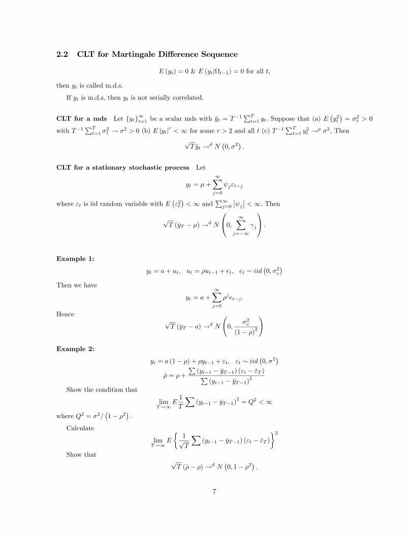
2.2 CLT for Martingale Di¤erence Sequence
E (yt) = 0 & E (ytjt�1) = 0 for all t;
then yt is called m.d.s.
If yt is m.d.s, then yt is not serially correlated.
CLT for a mds Let fytg1t=1 be a scalar mds with �yt = T�1PT
t=1 yt: Suppose that (a) E�y2t�= �2t > 0
with T�1PT
t=1 �2t ! �2 > 0 (b) E jytjr <1 for some r > 2 and all t (c) T�1
PTt=1 y
2t !p �2; Then
pT �yt !d N
�0; �2
�:
CLT for a stationary stochastic process Let
yt = �+1Xj=0
j"t�j
where "t is iid random variable with E�"2t�<1 and
P1j=0
�� j�� <1: ThenpT (�yT � �)!d N
0@0; 1Xj=�1
j
1A :
Example 1:
yt = a+ ut; ut = �ut�1 + et; et � iid�0; �2e
�Then we have
yt = a+
1Xj=0
�jet�j :
HencepT (�yT � a)!d N
0;
�2e
(1� �)2
!
Example 2:
yt = a (1� �) + �yt�1 + "t; "t � iid�0; �2
�� = �+
P(yt�1 � �yT�1) ("t � �"T )P
(yt�1 � �yT�1)2
Show the condition that
limT!1
E1
T
X(yt�1 � �yT�1)2 = Q2 <1
where Q2 = �2=�1� �2
�:
Calculate
limT!1
E
�1pT
X(yt�1 � �yT�1) ("t � �"T )
�2Show that
pT (�� �)!d N
�0; 1� �2
�:
7
Page 8
3 Finite Sample Properties
3.1 Calculating Bias By using Simple Taylor Expansion
Unknown Constant Case
yt = a+ �yt�1 + et; et � iidN (0; 1)
First, show that
E
�A
B
�=
EA
EB
1� Cov (A;B)
E(A)E(B)+V ar (B)
E (B)2
!+O
�T�2
�=
EA
EB� E (A� a) (B � b)
E(B)2+EAE (B � b)2
E (B)3 +O
�T�2
�Let EA = a; EB = b and take the Taylor expansion of A=B around a and b:
A
B=a
b+1
b(A� a)� a
b2(B � b)� 1
b2(A� a)(B � b)� 1
b2(A� a)(B � b) + a
b3(B � b)2 +Rn
Take expectation.
EA
B=
a
b+1
bE (A� a)� a
b2E (B � b)� 1
b2E (B � b) (A� a) + a
b3E (B � b)2 + ERn
=a
b� 1
b2Cov(A;B) +
a
b3V ar(B) +O
�T�2
�Now consider
E� = E
P~yt~yt�1P~y2t�1
=?
Note that in this example, we have
E (A) = E (B) =�2e
(1� �2) ��2e
T (1� �)2+O
�1
T 2
�and
E (xtxt+kxt+k+lxt+k+l+m) =�k+m
�1 + 2�2l
�(1� �2)2
if ut is normal.
From this, we can calculate all moments. For an example, we have
1
T 2E�X
x2t
�2=
1
T 2
"3T
(1� �2)2+ 2
T�1Xt=1
(T � i) 1 + 2�2t
(1� �2)2
#
Then we have �nally
E� = E
P~yt~yt�1P~y2t�1
= �� 1 + 3�T
+O�T�2
�so that
E (�� �) = �1 + 3�T
+O�T�2
�8
Page 9
For non-constant case
xt = �xt�1 + et
E (�� �) = �2�T+O
�T�2
�For a trend case
yt = a+ bt+ �yt�1 + et
E (�� �) = �2(1 + 2�)T
+O�T�2
�3.2 Approximating Statistical Inference by using Edgeworth Expansion
For non-constant case (Phillips, 1977), we have
�� � =Pyt�1utPy2t�1
=
Pyt�1 (yt � �yt�1)P
y2t�1=
Pyt�1yt � �
Py2t�1P
y2t�1
so that (�� �) can be expressed as a function of moments. Let
pT (�� �) =
pTe (m)
where m stands for a vector of moments. Then taking Taylor expansion yields
pTe (m) =
pT
�ermr +
1
2ersmrms +
1
6erstmrmsmt +Op
�1
T 2
��where
er =@e (0)
@mr; ... etc.
Solving all moments yields
Pr
pT (�� �)p1� �2
� w
!= �(w) +
� (w)pT
�p1� �2
!�w2 + 1
�where w = x=
p1� �2:
For constant case (Tanaka, 1983)
Pr
pT (�� �)p1� �2
� w
!= �(w) +
� (w)pT
�+ � (w)
2p1� �2
!
9
Page 10
4 Covariance-Stationary Vector Processes
Consider the following simple VAR(1) with bivariate variables
y1t = a1 + b11y1t�1 + b12y2t�1 + e1t
y2t = a2 + b21y1t�1 + b22y2t�1 + e2t;
alternatively we can rewrite it as
yt = a+ byt�1 + et
where
a =
24 a1
a2
35 ; b =
24 b11 b12
b21 b22
35 ; et =
24 e1t
e2t
35Usually,
Eete0s = for t = s
= 0 otherwise
4.1 State Space Representation
Consider VAR(p) with two variables given by
yt = a+ b1yt�1 + � � �+ bpyt�p + et
Then we can rewrite it as
26664yt � �...
yt�p+1 � �
37775 =
26666666664
b1 b2 � � � bp
I2 0 � � � 0
0 I2 � � � 0
. . .
0 0 � � � 0
37777777775
26664yt�1 � �
...
yt�p � �
37775+26666664et
0...
0
37777775 ;
or
�t = F�t�1 + vt
so that any VAR(p) can be rewritten as VAR(1). We call this form �state space representation�.
4.2 Stationarity Condition
The eigenvalues of the matrix F satisfy
��I�p�b1�p�1�b2�p�2� � � � � bp�� = 010
Page 11
where � are the eigenvalues. That is, as long as j�j < 1; yt is stationary.
Vector MA(1) Representation
If the eigenvalues of F all lie inside the unit circle, then F s ! 0 as s!1 and yt can be rewritten as
yt= �+1Xj=0
Fjvt�j
or equivalently
yt= �+1Xj=0
jet�j :
IfP1
j=0
�� j�� <1 (absolute summable), then
1. the autocovariance between the ith variable at time t and the jth variable s periods, E (yit � �i)�yjs � �j
�;
exisits and is given by the row i; column j element of
�s =1Xk=0
s+k 0k for s = 0; 1; :::
2. the sequence of matrices f�kg1k=0 is absolute summable
4.3 Autocovariance
Note that
Ey1ty1t�1 = Ey1ty1t+1;
Ey1ty2t�1 6= Ey1ty2t+1:
Let
E (yt) = �;
E (yt��) (yt�j��)0 = ��j
E (yt+j��) (yt��)0 = �j
and
��j 6= �j :
Similar to univariate case, we have
�yT! �;
and
limT!1
T � E�(�yT � �) (�yT � �)0
�=
1Xj=�1
�j 6= �0 + 21Xj=1
�j :
11
Page 12
4.4 Model Selection
Suppose that VAR(1) with two variables is a correct speci�cation. Then we have
y1t = a1 + b11y1t�1 + b12y2t�1 + e1t
= a1 + b11y1t�1 + b12 (a2 + b21y1t�2 + b22y2t�2 + e2t�1) + e1t
= a1 + a2b12 + b11y1t�1 + b12b21y1t�2 + e1t + b12e2t�1 + b22y2t�2
= a1 + a2b12 + b11y1t�1 + b12b21y1t�2 + e1t + e2t�1 + b22 (a2 + b21y1t�3 + b22y2t�3 + e2t�2)
...
= a+1Xj=1
bjy1t�j +1Xj=1
cje2t�j + e1t
so that we have AR(1). Similarly, if VAR(1) with three variables is a true model, then any two variables
have VAR(1).
Now consider the lag selection criteria.
AIC : cT (p) = ln����p���+ 21 + p
T
BIC : cT (p) = ln����p���+ 1 + p
TlnT
H-Q : cT (p) = ln����p���+ 21 + p
Tln lnT
For all three criteria, the lag length for each equation becomes identical. However it is not hard to conjecture
that single equation criteria can be used for selecting individual lag length.
Alternatively, GS method is also used here. However, there is no joint criteria available for GS method.
4.5 Finite Sample Properties
Let b =Pp
i=1 bi where bi is de�ned in
yt = a+ b1yt�1 + � � �+ bpyt�p + et:
The �rst order bias is studied by Nicholls and Pope (1988) given by
E�b� b
�= � 1
TC+O
�T�2
�where
C = G
24�I� b0��1 + b0 �I� b02��1 + pXj=1
�j (I��jb0)�135� (0)�1
and �j are the eigenvalues of b, and G is the covariance and variance matrix of et
Note that this formula is similar to panel VAR case which we will consider very soon.
12
Page 13
4.6 Granger Causality
There is no Granger Causality if
E (xt+sjxt; xt�1; � � � ) = E (xt+sjxt; xt�1; � � � ; yt; yt�1; � � � ) for all s > 0:
Testing: Under the null hypothesis of no Granger Causality (y2t to y1t), all upper o¤-diagonal elements
should be zero.
13
Page 14
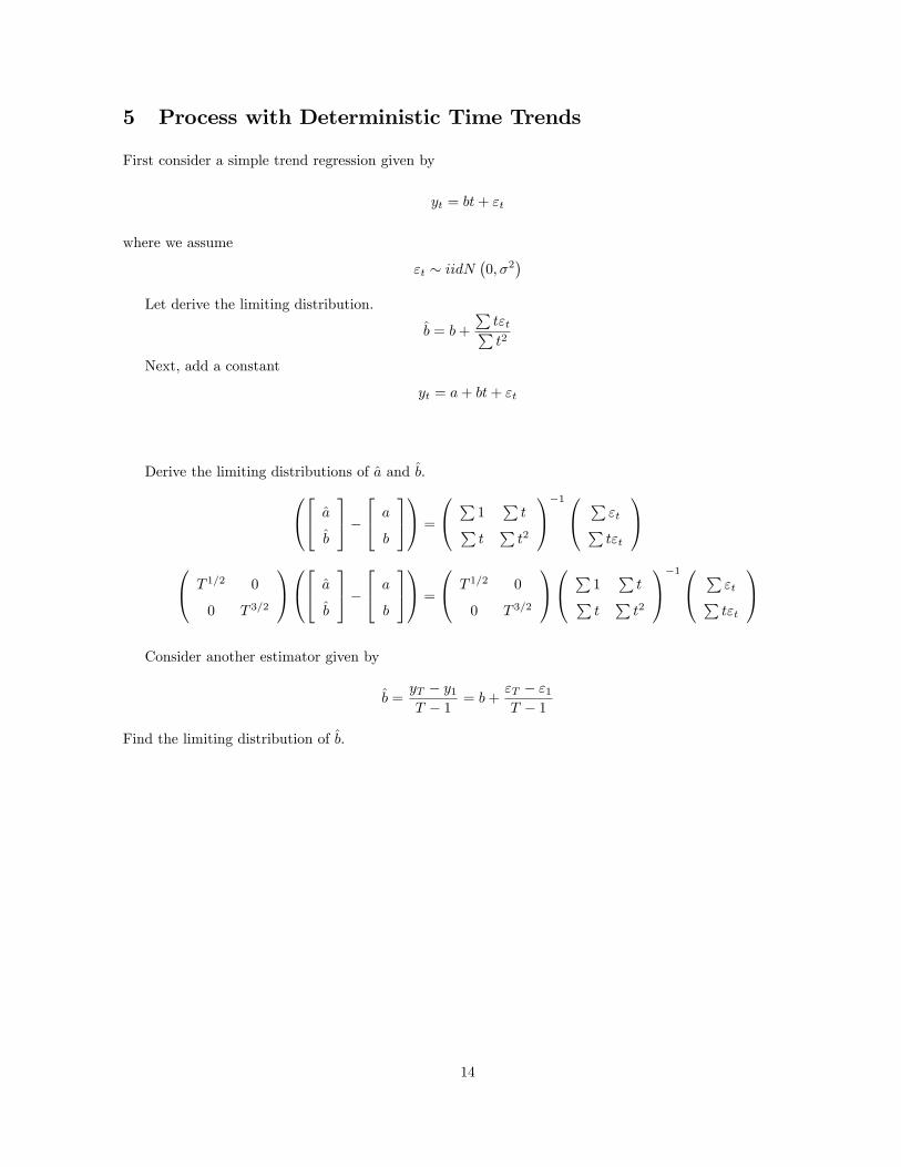
5 Process with Deterministic Time Trends
First consider a simple trend regression given by
yt = bt+ "t
where we assume
"t � iidN�0; �2
�Let derive the limiting distribution.
b = b+
Pt"tPt2
Next, add a constant
yt = a+ bt+ "t
Derive the limiting distributions of a and b:0@24 a
b
35�24 a
b
351A =
0@ P1
PtP
tPt2
1A�10@ P"tPt"t
1A0@ T 1=2 0
0 T 3=2
1A0@24 a
b
35�24 a
b
351A =
0@ T 1=2 0
0 T 3=2
1A0@ P1
PtP
tPt2
1A�10@ P"tPt"t
1AConsider another estimator given by
b =yT � y1T � 1 = b+
"T � "1T � 1
Find the limiting distribution of b:
14
Page 15
6 Univariate Processes with Unit Roots
yt = a+ ut; ut = ut�1 + "t
Then we have
yt = yt�1 + "t
Let
yt = "1 + � � �+ "t
where
"t � iidN (0; 1)
Then we have
yt � N (0; t)
and
yt � yt�1 = "t � N (0; 1)
yt � ys � N (0; t� s)
Rewrite as a continuous time stochastic process such that
Standard Brownian Motion: W (�) is a continuous-time stochastic process, associatting each date t 2
[0; 1] with the scalar W (t) such that
1. W (0) = 0
2. [W (s)�W (t)] � N (0; s� t)
3. W (1) � N (0; 1)
Transition from discrete to continuous. First let "t � iidN (0; 1)
1pT
1
T
TXt=1
yt =1pT
TXt=1
ytT=
1pT
"1T+"1 + "2T
+ � � �+ 1
T
TXt=1
"t
!
! d
Z 1
0
W (r) dr
1
T 2
TXt=1
y2t !d
Z 1
0
W 2dr
15
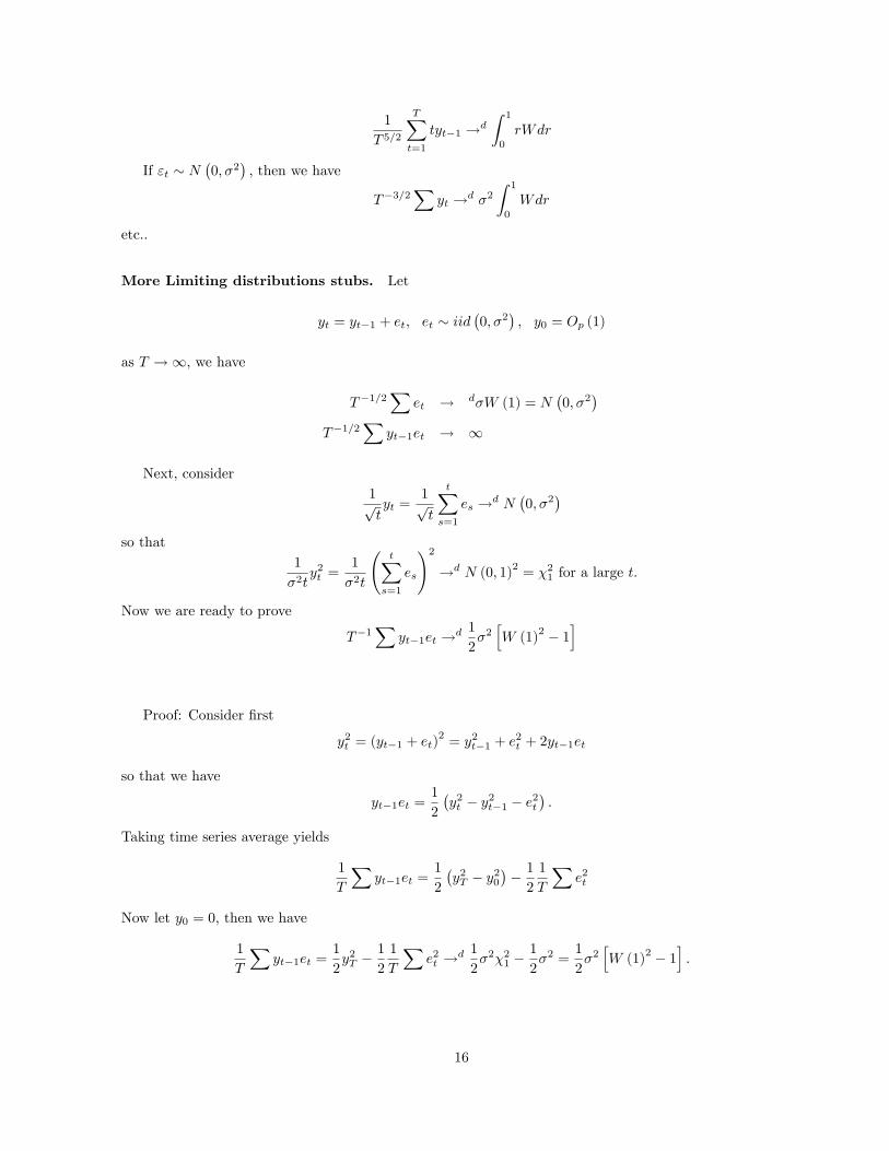
Page 16
1
T 5=2
TXt=1
tyt�1 !d
Z 1
0
rWdr
If "t � N�0; �2
�; then we have
T�3=2X
yt !d �2Z 1
0
Wdr
etc..
More Limiting distributions stubs. Let
yt = yt�1 + et; et � iid�0; �2
�; y0 = Op (1)
as T !1; we have
T�1=2X
et ! d�W (1) = N�0; �2
�T�1=2
Xyt�1et ! 1
Next, consider1ptyt =
1pt
tXs=1
es !d N�0; �2
�so that
1
�2ty2t =
1
�2t
tX
s=1
es
!2!d N (0; 1)
2= �21 for a large t:
Now we are ready to prove
T�1X
yt�1et !d 1
2�2hW (1)
2 � 1i
Proof: Consider �rst
y2t = (yt�1 + et)2= y2t�1 + e
2t + 2yt�1et
so that we have
yt�1et =1
2
�y2t � y2t�1 � e2t
�:
Taking time series average yields
1
T
Xyt�1et =
1
2
�y2T � y20
�� 12
1
T
Xe2t
Now let y0 = 0; then we have
1
T
Xyt�1et =
1
2y2T �
1
2
1
T
Xe2t !d 1
2�2�21 �
1
2�2 =
1
2�2hW (1)
2 � 1i:
16
Page 17
Next, consider
1
T 3=2
Xyt�1 =
1
T 3=2(e1 + (e1 + e2) + � � �+ (e1 + � � �+ eT�1))
=1
T 3=2((T � 1) e1 + (T � 2) e2 + � � �+ eT�1)
=1
T 3=2
TXt=1
(T � t) et =1
T 1=2
TXt=1
et �1
T 3=2
TXt=1
tet:
Now we are ready to prove
T�3=2X
tet !d �W (1)� �Z 1
0
W (r) dr
Proof:
T�3=2X
tet =1
T 1=2
TXt=1
et �1
T 3=2
Xyt�1 !d �W (1)� �
ZW (r) dr:
Questions:
1. Consider this
yt = yt�1 + et; ut � iid�0; �2u
�: Eetus = 0 for all t; s:
Then derive the limiting distribution of
T�1X
yt�1ut
2. Prove the followings
(a) T�5=2Ptyt�1 !d �
RrW (r) dr
(b) T�3Pty2t�1 !d �
RrW (r)
2dr
6.1 Limiting Distribution of Unit Root Process I (No constant)
Consider the simple AR(1) regression without constant,
yt = �yt�1 + et:
Then OLS estimator is given by
�� � =Pyt�1etPy2t�1
When � = 1; we know
1
T
Xyt�1et ! d 1
2�2hW (1)
2 � 1i;
1
T 2
TXt=1
y2t ! d�2Z 1
0
W 2dr:
17
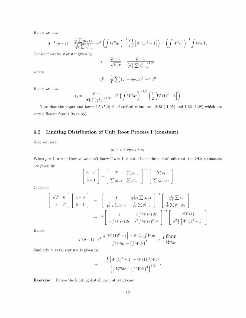
Page 18
Hence we have
T�1 (�� 1) =1T
Pyt�1et
1T 2
Py2t�1
!d
�ZW 2dr
��1�1
2
hW (1)
2 � 1i�=
�ZW 2dr
��1 ZWdW:
Consider t-ratio statistic given by
t� =�� 1p��T
=�� 1�
�2TPy2t�1
�1=2where
�2T =1
T
X(yt � �yt�1)2 !p �2
Hence we have
t� =�� 1�
�2TPy2t�1
�1=2 !d
�ZW 2dr
��1=2�1
2
hW (1)
2 � 1i�
Note that the upper and lower 2.5 (5.0) % of critical values are -2.23 (-1.95) and 1.62 (1.28) which are
very di¤erent from 1.96 (1.65).
6.2 Limiting Distribution of Unit Root Process I (constant)
Now we have
yt = a+ �yt�1 + et
When � = 1; a = 0: Howeve we don�t know if � = 1 or not. Under the null of unit root, the OLS estimators
are given by 24 a� 0
�� 1
35 =24 T
Pyt�1P
yt�1Py2t�1
35�1 24 PetP
yt�1et
35Consider24 p
T 0
0 T
3524 a� 0
�� 1
35 =
24 1 1T 3=2
Pyt�1
1T 3=2
Pyt�1
1T 2
Py2t�1
35�1 24 1pT
Pet
1T
Pyt�1et
35! d
24 1 �RW (r) dr
�RW (r) dr �2
RW (r)
2dr
35�1 24 �W (1)
�2 12
hW (1)
2 � 1i 35
Hence
T (�� 1)!d
12
hW (1)
2 � 1i�W (1)
RWdrR
W 2dr ��RWdr
�2 =
R~WdWR~W 2dr
Similarly t�ratio statistic is given by
t� !d
12
hW (1)
2 � 1i�W (1)
RWdrnR
W 2dr ��RWdr
�2o1=2 :
Exercise: Derive the limiting distribution of trend case.
18
Page 19
6.3 Unit Root Test
For AR(p), we have
yt = a+ �yt�1 +X
�j�yt�j + et
Note that1
T
X�yt�j = Op
�1pT
�;
so that as T !1; the augmented term goes away. Hence the limiting distribution does not change at all.
7 Meaning of Nonstationary
Let�s �nd an economic meaning of nonstationarity.
1. No steady state. No static mean or average exists. A series becomes random around its true mean.
Never converge to its mean.
2. No equilibrium since there is no steady state. Cannot forecast or predict its future value without
considering other nonstationary variable.
3. Fast convergence rate.
7.1 Unit Root Test and Stationarity Test
Note that the rejection of the null of unit root does not imply that a series is stationary. To see this, let
xt = �xt�1 + "t; "t =ptet; et � iid
�0; �2
�:
Further let � = 0: Now xt is not weakly stationary since its variance is time varying. However at the same
time, xt does not follow unit root process since � = 0: To see this, let derive the limiting distribution of �:
�� � =Pxt�1"tPx2t�1
and
E�X
xt�1"t
�2= E
�X"t�1"t
�2= E
�Xtet�1et
�2=
��2�2 T 2
2+O (T )
so that1
T
Xxt�1"t !d N
�0;�4
2
�
19
Page 20
Xx2t�1 =
X"2t�1 =
Xte2t�1 !p �2
T 2
2+O (T )
Hence we have
T (�� �) =1T
Pxt�1"t
1T 2
Px2t�1
!d N (0; 2) =p2W (1) :
Therefore, we can see that the convergence rate is still T; but the limiting distribution is not a function of
Brownian motion at all.
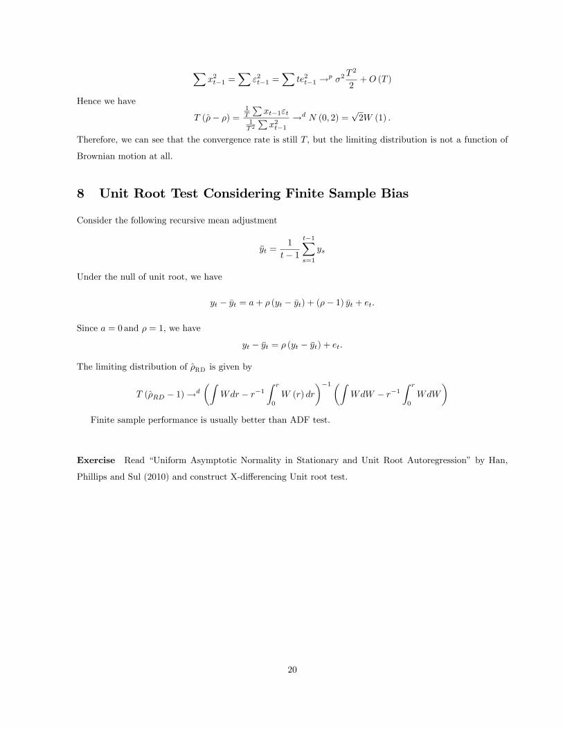
8 Unit Root Test Considering Finite Sample Bias
Consider the following recursive mean adjustment
�yt =1
t� 1
t�1Xs=1
ys
Under the null of unit root, we have
yt � �yt = a+ � (yt � �yt) + (�� 1) �yt + et:
Since a = 0 and � = 1; we have
yt � �yt = � (yt � �yt) + et:
The limiting distribution of �RD is given by
T (�RD � 1)!d
�ZWdr � r�1
Z r
0
W (r) dr
��1�ZWdW � r�1
Z r
0
WdW
�Finite sample performance is usually better than ADF test.
Exercise Read �Uniform Asymptotic Normality in Stationary and Unit Root Autoregression� by Han,
Phillips and Sul (2010) and construct X-di¤erencing Unit root test.
20
Page 21
9 Weak Stationary and Local to Unity
Joon Park (2007) and Phillips and Magdalinos (2007, JoE)
Consider the following DGP
yt = �nyt�1 + ut; t = 1; :::; n;
where
�n = 1�c
n�; 0 � � < 1 and c > 0
Then we havepn (�n � �n)!d N
�0; 1� �2n
�so that p
np1� �2n
(�n � �n)!d N (0; 1) :
Note that
1� �2n = 1� 1 +c2
n2�+2c
n�=
c2
n2�+2c
n�= O
�n��
�+O
�n�2�
�;
hence p1� �2n =
r2c
n�
�1 +
c
2n�
�;
and pnp
1� �2n= n1=2n�=2
1p2c+O
�n�+1=2
�:
Finally we have
n�+12 (�n � �n)!d N (0; 2c)
For the case of � = 1; we call it local to unity of which limiting distribution is di¤erent. (Phillips 1987,
Biometrica, 88 Econometrica). Consider the following simple DGP
yt = �nyt�1 + ut; �n = exp� cT
�' 1 + c
T
Now, de�ne
J (r) =
Z r
0
e(r�s)cdW (s)
where J (r) is a Gaussian process which for �xed r > 0; has the distribution
J (r) � N
�0;1
2
e2rc � 1c
�;
and it call Ornstein-Uhlenbeck process. Alternatively we have
J (r) =W (r) + c
Z r
0
e(r�s)cW (s) ds:
21
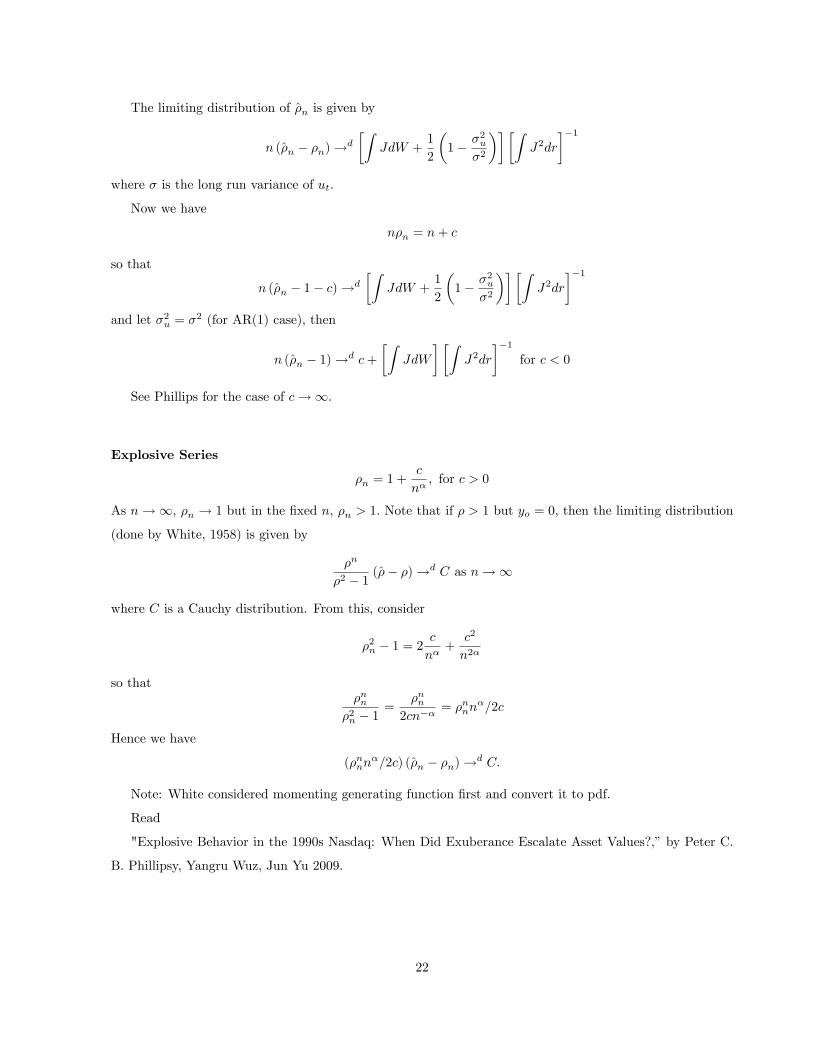
Page 22
The limiting distribution of �n is given by
n (�n � �n)!d
�ZJdW +
1
2
�1� �2u
�2
���ZJ2dr
��1where � is the long run variance of ut:
Now we have
n�n = n+ c
so that
n (�n � 1� c)!d
�ZJdW +
1
2
�1� �2u
�2
���ZJ2dr
��1and let �2u = �2 (for AR(1) case), then
n (�n � 1)!d c+
�ZJdW
� �ZJ2dr
��1for c < 0
See Phillips for the case of c!1:
Explosive Series
�n = 1 +c
n�; for c > 0
As n!1; �n ! 1 but in the �xed n; �n > 1: Note that if � > 1 but yo = 0; then the limiting distribution
(done by White, 1958) is given by
�n
�2 � 1 (�� �)!d C as n!1
where C is a Cauchy distribution. From this, consider
�2n � 1 = 2c
n�+
c2
n2�
so that�nn
�2n � 1=
�nn2cn��
= �nnn�=2c
Hence we have
(�nnn�=2c) (�n � �n)!d C:
Note: White considered momenting generating function �rst and convert it to pdf.
Read
"Explosive Behavior in the 1990s Nasdaq: When Did Exuberance Escalate Asset Values?,�by Peter C.
B. Phillipsy, Yangru Wuz, Jun Yu 2009.
22
Page 23
10 Cointegration
10.1 Multivariate Integrated Process (Chap 18)
Let
yt= yt�1+ut
where yt is a vector of nonstationary process. We further assume that
ut =1Xs=1
s"t�s
whereP1
s=0 s�� sij�� <1. Let E ("t"0t) = ; then
�s = E�utu
0t�s�=
1Xv=0
s+v 0v:
Further de�ne
= PP0
and
(1) = 0+ 1 + � � � ;
� = (1)P
Then we have
T�1=2X
ut !d �W (1)
23
Page 24
T�1X
yt�1u0t ! d�
�ZWdW
��0 +
1Xv=1
�0v
T�3=2X
yt�1y0t�1 ! d�
�ZWW0dr
��0
We are ready to analyze time series regression with integrated processes. Consider
yt = �xt + ut; ut = ut�1 + "t
Then we have �� � �
�=�X
x2t
��1 �Xxtut
�!d?
To �nd out this, we can choose two ways. The �rst way is to de�ne the bivariate process of yt and xt: By
doing this, we can know what � stands for. See Hamilton p. 558-559. The second way is just considering
the following results. Let
zt = (xt; ut)0;
then
T�3=2X
ztz0t =
0@ T�3=2Px2t T�3=2
Pxtut
T�3=2Pxtut T�3=2
Pu2t
1A!d
0@ �11RW 21 �12
RW1W2
�12RW1W2 �22
RW 22
1Awhere � can be de�ned as
�zt= (L) "t
and
� = (1)P; and ��0= �:
Now consider the rate of convergence. Since ut is I(1) ;Pxtut is needed to divide by T 3=2 and
Px2t as
well. Hence the rate of convergence is 1. What does it mean then?
10.2 Common Factor across Variables
Consider a process given by
yt = ��t + ut; �t = �t�1 +mt; ut � iidN (0; 1) :
Note that yt is I (1) : Next, consider a similar process of which contains �t:
xt = �t + "t; "t � iidN (0; 1) :
Then we have
yt � �xt = ut � �"t = I (0) :
In this case, we say yt is cointegrated with xt:
24
Page 25
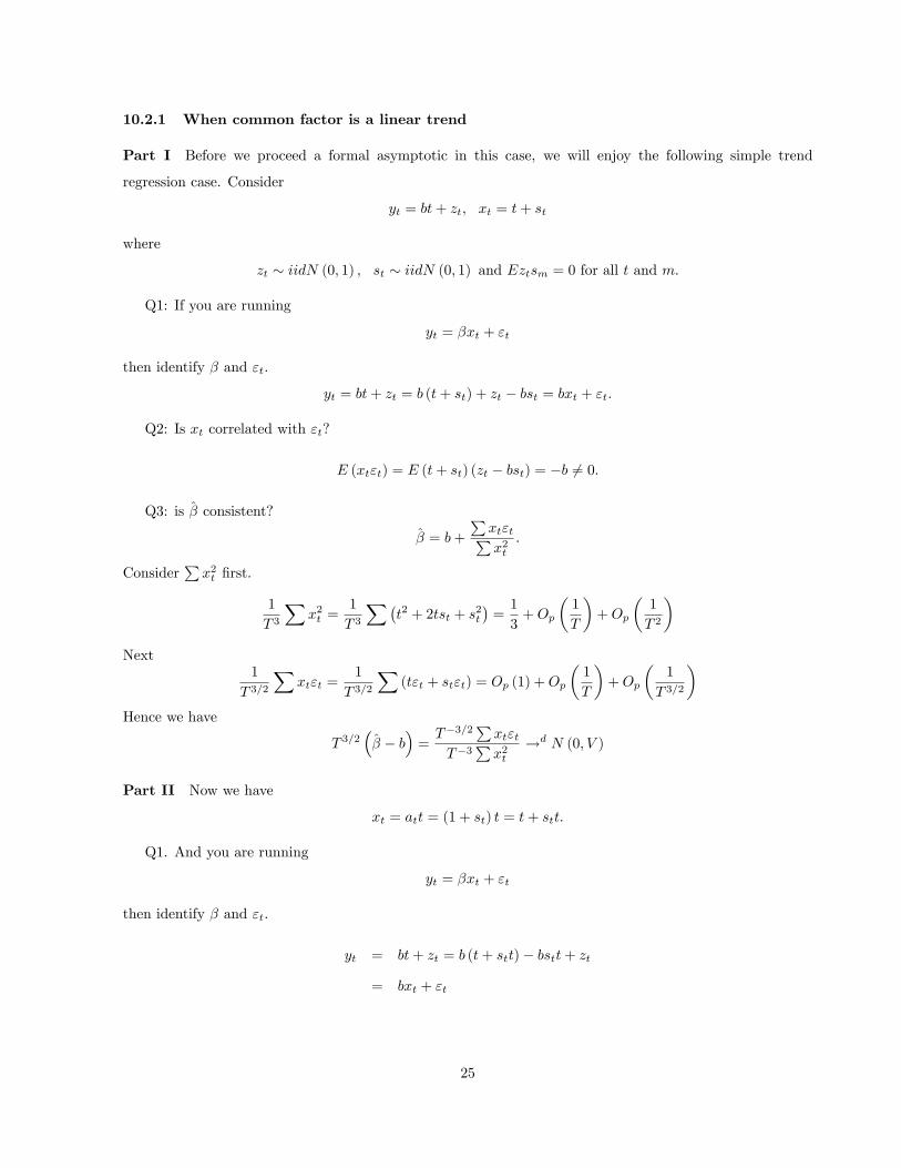
10.2.1 When common factor is a linear trend
Part I Before we proceed a formal asymptotic in this case, we will enjoy the following simple trend
regression case. Consider
yt = bt+ zt; xt = t+ st
where
zt � iidN (0; 1) ; st � iidN (0; 1) and Eztsm = 0 for all t and m:
Q1: If you are running
yt = �xt + "t
then identify � and "t:
yt = bt+ zt = b (t+ st) + zt � bst = bxt + "t:
Q2: Is xt correlated with "t?
E (xt"t) = E (t+ st) (zt � bst) = �b 6= 0:
Q3: is � consistent?
� = b+
Pxt"tPx2t
:
ConsiderPx2t �rst.
1
T 3
Xx2t =
1
T 3
X�t2 + 2tst + s
2t
�=1
3+Op
�1
T
�+Op
�1
T 2
�Next
1
T 3=2
Xxt"t =
1
T 3=2
X(t"t + st"t) = Op (1) +Op
�1
T
�+Op
�1
T 3=2
�Hence we have
T 3=2�� � b
�=T�3=2
Pxt"t
T�3Px2t
!d N (0; V )
Part II Now we have
xt = att = (1 + st) t = t+ stt:
Q1. And you are running
yt = �xt + "t
then identify � and "t:
yt = bt+ zt = b (t+ stt)� bstt+ zt
= bxt + "t
25
Page 26
Q2: Is xt correlated with "t?
E (xt"t) = E (t+ st) (zt � bstt) = Ebs2t t = bt 6= 0
Q3: is � consistent?
E1
T 3
Xx2t = E
1
T 3
Xt2 (1 + st)
2= E
1
T 3
Xt2�1 + s2t + 2st
�=
1
3O (1) +O
�1
T
�+O
�1
T 2
�Next
EX
xt"t =?
Derive it.
10.2.2 When the common factors are stochastic.
Consider the following processes again
yt = ��t + ut; �t = �t�1 +mt; ut � iidN (0; 1) ; mt � iidN�0; �2
�:
We assume further that
Emtus = 0 for all t and s:
Let�s derive the limiting distribution of
1
T 3=2
X�tut:
First its mean is zero. Next,
E�X
�tut
�2= E
��21u
21 + :::+ �
2Tu
2T
�= �2 (1 + 2 + :::+ T ) =
�2
2T 2 +O (T )
Hence we have1
T
X�tut !d N
�0;�2
2
�:
Now consider
yt = ��t + ut; xt = �t + et;
Then
Q1: If you are running
yt = �xt + "t
then identify � and "t:
yt = ��t + ut = � (�t + et) + ut � �et = bxt + "t:
26
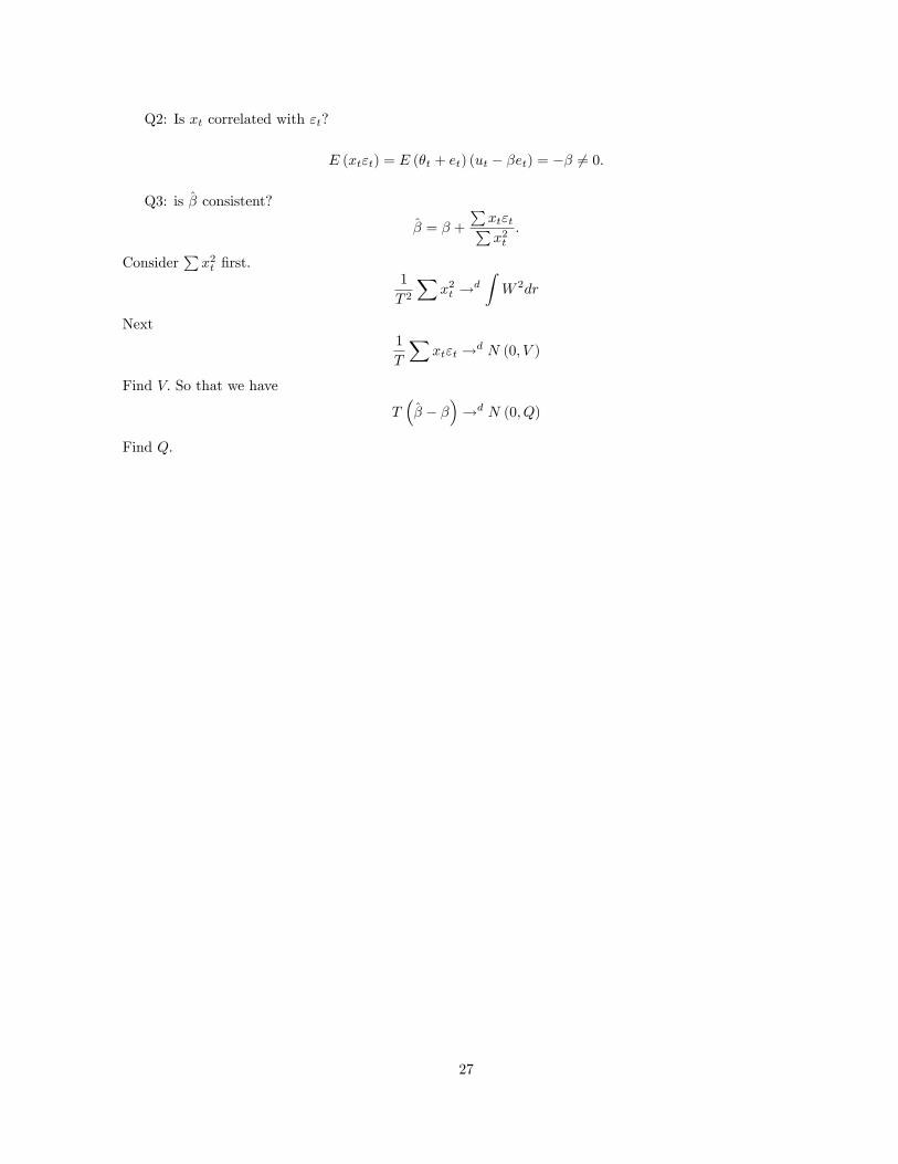
Page 27
Q2: Is xt correlated with "t?
E (xt"t) = E (�t + et) (ut � �et) = �� 6= 0:
Q3: is � consistent?
� = � +
Pxt"tPx2t
:
ConsiderPx2t �rst.
1
T 2
Xx2t !d
ZW 2dr
Next1
T
Xxt"t !d N (0; V )
Find V: So that we have
T�� � �
�!d N (0; Q)
Find Q:
27
Page 28
11 Cointegration Test
Consider a simple case
yt = �xt + ut; ut = ut�1 + "t
where xt is independent from ut: Let
ut = yt � �xt
and run
ut = �ut�1 + et
Then
Z� = T (�� 1) =1T
Put�1et
1T 2
Pu2t�1
Note that
ut = yt ��P
xtytPx2t
�xt
Let
Q (r) =Wy (r)�ZWyW
0x
�ZWxW
0x
��1Wx (r)
Then we have1
T 2
Xu2t�1 !d
Z 1
0
Q (r)2dr
and1
T
Xut�1et !d
Z 1
0
Q (r) dR
Hence �nally
Z� !d
�ZQ (r) dR
��Z 1
0
Q (r)2dr
��1:
Note htat Q (r) is depending on the value of �. Intutitively, we can say that we have more regressors,
the variability of � will increase so that the quantity of Q (r) is also increasing. That is, for two regressors
case, we have
ut = yt � �1x1t � �2x2t =��1 � �1
�x1t +
��2 � �2
�x2t:
Therefore, the limiting distribution is depending on the number of regressors. As more regressors enters, the
critical value is getting larger.
12 Error Correction Model (ECM)
Here I introduce ECM in an intuitive way. Consider the case of cointegration �rst. Then we have
ut = �ut�1 + et
28
Page 29
or
�ut = (�� 1)ut�1 + et
or
�yt � ��xt = (�� 1) (yt�1 � �xt�1) + et:
This regression model can be further decomposed into
�yt = �1 (yt�1 � �xt�1) + e1t
�xt = �2 (yt�1 � �xt�1) + e2t
and
�1 � ��2 = �� 1:
Note that the lagged term is call �error correction�term, and so it call error correction model.
If ut follows AR(p), then the general ECM is given by
�yt = �1 (yt�1 � �xt�1) +p�1Xj=1
�yj�yt�j +
p�1Xj=1
�xj�xt�j + e1t;
�xt = �1 (yt�1 � �xt�1) +p�1Xj=1
�yj�yt�j +
p�1Xj=1
�xj�xt�j + e1t:
Now let�s compare no-cointegration case. If yt is not cointegrated with xt; we have
�yt =
p�1Xj=1
�yj�yt�j +
p�1Xj=1
�xj�xt�j + e1t;
�xt =
p�1Xj=1
�yj�yt�j +
p�1Xj=1
�xj�xt�j + e1t:
so that there is no error correction term in the VAR system.
13 Midterm Exam
1. Find AR order.
2. Test Granger Causality (assume y and x are stationary). Use bootstrap critical values.
3. Test unitroot.
4. Test cointegration.
5. Run ECM.
29


![South African Astronomical Observatory · 2019. 9. 17. · y]t w w d t\y y t uu d z yy yyv y v t&[y sv y u yv x w v [y ut w y s y s w yw uv s zd []w y]t w z&d sw y y t uu d st v yyv](https://static.documents.pub/doc/80x56/60b7194c54d6b33e0b48e0ce/south-african-astronomical-observatory-2019-9-17-yt-w-w-d-ty-y-t-uu-d-z-yy.jpg)


