1 Statistical Analysis of Signal-Dependent Noise ...

1

Statistical Analysis of Signal-Dependent Noise:Application in Blind Localization of Image

Splicing ForgeryMian Zou, Heng Yao, Member, IEEE , Chuan Qin, Xinpeng Zhang, Member, IEEE

Abstract—Visual noise is often regarded as a disturbance in image quality, whereas it can also provide a crucial clue for image-based forensic tasks. Conventionally, noise is assumed to comprise an additive Gaussian model to be estimated and then used toreveal anomalies. However, for real sensor noise, it should be modeled as signal-dependent noise (SDN). In this work, we apply SDNto splicing forgery localization tasks. Through statistical analysis of the SDN model, we assume that noise can be modeled as aGaussian approximation for a certain brightness and propose a likelihood model for a noise level function. By building a maximum aposterior Markov random field (MAP-MRF) framework, we exploit the likelihood of noise to reveal the alien region of spliced objects,with a probability combination refinement strategy. To ensure a completely blind detection, an iterative alternating method is adopted toestimate the MRF parameters. Experimental results demonstrate that our method is effective and provides a comparative localizationperformance.

Index Terms—Signal-dependent noise, likelihood model, splicing forgery localization, MAP-MRF, iterative alternating method, blinddetection.

F

1 INTRODUCTION

DURING the process of acquisition or transmission, vi-sual signals are often distorted by various types of dis-

turbance, including noise, blur, enhancement, etc. Amongthese, noise is among the most common. Moreover, noiseis inevitably incurred during visual information acquisition[1], such as digital photography under low light condition.Many works have explored how to estimate the noise andremove noise to improve visual quality. However, noise isnot always useless; for example, it is beneficial in imageforensics, especially in image splicing forgery localization,when it does not interfere with the visual experience. As isgenerally known, the wide availability of powerful imageediting tools has made image manipulation easier, which islikely to trigger severe consequences in individuals’ sociallife. In this context, investigating detection algorithms isworthwhile, including approaches based on intrinsic noiseinside different cameras, of image malicious manipulation.

Noise estimation lays crucial groundwork for noise-based blind image forensic algorithms. Most existing meth-ods of noise estimation assume additive white Gaussiannoise (AWGN), in which noise is represented by a fixed

• M. Zou is with School of Mechanical Engineering, University of Shanghaifor Science and Technology, Shanghai 200093, China.E-mail: [email protected].

• H. Yao and C. Qin are with School of Optical-Electrical and ComputerEngineering, University of Shanghai for Science and Technology, Shang-hai 200093, China.E-mail: [email protected]; [email protected].

• X. Zhang is with School of Computer Science, Fudan University, Shang-hai 200433, China.E-mail: [email protected].

Manuscript received Oct 30, 2020. This work was supported by the NationalNatural Science Foundation of China (61702332, 61672354, U1936214,U1636206, and 61525203.) (Corresponding author: Heng Yao.)

standard deviation given a single noisy image. In [2]–[5],researchers estimated the noise level by solving a nonlinearprogramming problem with respect to high-order imagestatistics, such as kurtosis and skewness. Instead of analyz-ing statistical properties, some approaches are patch-based.In [6], Pyatykh et al. applied principle component analysis(PCA) to selected patches, estimating the noise intensityfrom the minimum eigenvalue of the covariance matrix.More recently, Wu et al. [7] estimated the noise level byexploiting irregular-shaped patches based on a superpixelscheme. However, AWGN conjecture does not hold for real-life digital photographs because actual CCD/CMOS sensornoise is strongly dependent on brightness. Thus, noise isbetter modeled as signal-dependent noise (SDN), where thenoise standard deviation can be represented as a functionof brightness. In [8], Foi et al. modeled the SDN as Poisson-Gaussian noise, where signal-dependent noise was repre-sented by a Poisson model while the signal-independentcomponent was demonstrated by a Gaussian model. Donget al. [9] proposed an effective SDN estimation method, inwhich regions with a frequently occurring intensity wereselected to estimate the noise via constrained weight least-squares. Meanwhile, the investigators proposed in [10]–[14]that noise distribution for the radiance of each scene waslikely to be skewed due to non-linear processing in the im-age sensor, which could be referred to as a camera responsefunction (CRF). Accordingly, based on the observation ofskewed noise, Liu et al. [15] modeled the sensor noise fromthe irradiance domain and converted the signal into theintensity domain using pre-measured CRF. This methodassumed a piecewise smooth model, estimating noise by theway of Bayesian inference. This work was further extendedin [16], [17], where Yang et al. introduced a sparse modelfor sensor noise, both in terms of estimation and denoising.

arX

iv:2

010.

1621

1v2

[cs

.CV

] 2

Nov

202

0

2

Additionally, Thai et al. [18] improved the Poisson-Gaussianmodel by employing gamma-correction to represent non-linearity.

Detecting and locating a splicing forgery in a digitalimage are usually based on the exposed significant vari-ations of intrinsic characteristics that would otherwise beconsistent in an untampered image. Noise or noise-relatedfeatures can be used as a significant clue for distinguishingorigins in a composited image due to its inevitable occur-rence during the in-camera processing. Existing methodscan be simply categorized into three classes: blind meth-ods, prior information-needed methods, and deep learning-based methods.

Blind methods do not use any external data for trainingor other pre-processing, relying exclusively on the imageitself to reveal the presence of manipulation. In [19], thenoise variance was estimated by applying wavelet analysisto non-overlapping image blocks, and then a segmentationprocess was carried out to check for homogeneity. In [20],Lyu et al. proposed a blind noise estimation approach toevaluate the noise level using projection kurtosis, and thendesigned a splicing detection method based on blind localvariance estimation. Yao et al. [21] also adopted the relationof projection kurtosis and noise to expose splicing forgery,incorporating an inhomogeneity scoring strategy to handlethe impact of the complexity of the texture. Zeng et al. [22]utilized the K-means clustering method to classify originaland suspicious regions according to the block noise varianceobtained by a PCA-based method [6]. Unlike the aboveapproaches, which assumed a constant noise level imposedby the AWGN model across an untampered image, recentworks have used an intensity-dependent noise model. In[23], Pun et al. proposed a Poisson model to indicate theprimitiveness of noise artifacts based on noise level function(NLF) to reveal splicing. Yao et al. [24] found inconsistencyin noise level functions in different regions of a test aimedto locate splicing forgery. In [25], Zhu et al. adopted an NLFto reflect the relationship between noise variance and thesharpness of block, generating a distance map for splicingdetection. It is also worth mentioning that in [26], localnoise variance was estimated by an adaptive SVD with anSVM training, which was exploited to find inconsistency.Another approach to exploit noise is the residual-basedmethod. In [27], the high-pass noise residuals of an imagewere exploited to extract rich features; next, the expectationmaximization (EM) algorithm was then applied to revealanomalies.

A photo-response non-uniformity (PRNU) noise pattern,which can be categorized as a prior information-neededmethod, has also been widely studied. Chen et al. [28]estimated the predictor of PRNU and noise residuals, thenincorporated a decision test into a binary hypothesis prob-lem. Korus et al. [29] proposed a PRNU-based tamperinglocalization method using a multi-scale fusion approach.In turn, Cozzolino et al. [30] proposed a blind localizationmethod; however, it still needs an image dataset in advancefor the clustering module. As an alternative, deep learning-based methods have commanded much attention in recentyears. Barni et al. [31] proposed a CNN-based approach,which worked on noise residuals to expose double JPEGcompression traces. Bondi et al. [32] exploited CNN to

extract characteristic camera model features from imagepatches and then localized the alien region employing it-erative clustering techniques. More recently, Cozzolino et al.[33] proposed a novel deep learning method to extract anoise residual, called noiseprint, for various forensic tasks,especially in image forgery localization. Generally, meth-ods that require prior information and deep learning-basedmethods must meet the prerequisite that a large number ofauthentic images are available, which are known to comefrom the camera of interest, or image training datasetsmust be prepared in advance. However, such a scenariois not always reasonable in the real world, in which mostdetection scenarios are blind. Meanwhile, deep learning-based methods may be affected by any variation in thedatasets during the test.

Since the noise level is dependent on image brightness,we used NLF to represent the noise characteristic of an im-age. We first proposed a conditional probability model usingchi-square distribution, which was based on an approximateGaussian model, to handle the different intensities of aliennoise, considering non-linearity and signal-dependency atthe same time. Meanwhile, physical properties in a neigh-borhood of image space were taken into account with aMarkov random field (MRF), which could overcome thedefects resulting from individual impact of noise inten-sity. We further inferred the forgery location map usingthe maximum a posterior (MAP)-MRF framework, allowingthe final decision map to be object-orientated and edge-smooth. Experiments were conducted to demonstrate thatour approach outperformed other noise-based localizationmethods, yielding results that were both quantitatively con-vincing and visually pleasing. Moreover, our approach isdistinctively automatic and blind to all images. The mainhighlights of this work can be summarized as follows:

1) We proposed a statistical assumption of signal-dependent noise, and analyzed the statistical char-acteristic of NLF, providing empirical evidence.

2) We introduced the MAP-MRF framework to blindlydetect the splicing forgery with a conditional likeli-hood model between original noise and alien noise.

3) We solved the MRF parameters estimation via an it-erative alternating strategy without any supervisedtraining.

The paper is organized as follows: Section 2 analyzesthe statistical characteristics of NLF and provides empiricalevidences. Section 3 details the method for localizing asplicing forgery based on NLF and MAP-MRF, with experi-mental results shown in Section 4. Finally, Section 5 providesconcluding remarks.

2 STATISTICAL ANALYSIS OF SIGNAL-DEPENDENTNOISE

2.1 Image noise modeling and analysisLet y ∈ R be a digital image, defined on a rectangular latticeΩ, with yi ∈ Ω, observed at the camera output, either as asingle-color band or a composition of multiple color bands.Let us suppose, in a simplified model [34], that y can bewritten as

y = x+ n, (1)

ZOU et al.: STATISTICAL ANALYSIS OF SIGNAL-DEPENDENT NOISE: APPLICATION IN BLIND LOCALIZATION OF IMAGE SPLICING FORGERY 3

Atmospheric

Attention

Lens/Geometric

Distortion

CCD Imaging/

Bayer Pattern

Fixed Pattern

Noise

Dark Current

Noise

Thermal

Noise

tInterpolation/

Demosaic

White

Balance

Gamma

CorrectionA/D Converter

Quantization

Noise

Dark Current

Noise

Fig. 1. Imaging pipeline of CCD/CMOS camera, redrawn from [15].

where x is the ideal noise-free image, while n is the noisethat accounts for all types of disturbance. Inside a cam-era, although the additive Gaussian noise model is widelyassumed, noise exhibits signal-dependent behavior andgreatly relies on the non-linear camera response function(CRF). According to [15], the noise model takes the form

x = f(L),y = f(L+ ns + nc) + nq,

(2)

where f (·) is the CRF; ns denotes all the noise componentsthat depend on irradiance L, that is, ns ∼ N (0, Lσ2

s); ncis the independent noise that is assumed nc ∼ N (0, σ2

c );and nq is the additional quantization noise, which canbe ignored in the model since it is quite small comparedwith other noise. Providing a better describe description ofthe noise characteristics inside a camera [15], the NLF is

estimated as σ (x) =√E (y − x)

2. The estimation of NLFcan be further rewritten as

σ (x) =

√E (f (f−1 (x) , f, σs, σc)− x)

2, (3)

where σs and σc are the standard deviation of ns and nc,respectively.

Based on [15], we know that CRF dominates the shapeof NLF; σs and σc dominate the numerical values in everyintensity of NLF. In the following, we would like to studythe influence of σs and σc in detail. Neglecting the CRF,noisy image y can be modeled as the sum of x, ns and nc,while x is equivalent to irradiance L. Thus, the variance ofy can be derived as

σ2(y) = σ2(x) + σ2(ns) + σ2(nc) = xσ2s + σ2

c . (4)

Therefore, noise statistics for y can be expressed as y ∼N (x, xσ2

s + σ2c ), by which (1) can also be rewritten as

y ≈ x+√xσ2

s + σ2c × ξn, (5)

where ξn stands for a variable with standard normal dis-tribution, i.e., ξn ∼ N (0, 1). From (5), the assumption thatnoise is additive Gaussian noise model is farfetched. Onlywhen x is very small, which means xσ2

s may be negligible,is the noise level dominated by nc, and the noise model canbe assumed to be approximately Gaussian. However, xσ2

s

cannot be ignored when x is large; therefore the noise levelis determined by ns and nc simultaneously.

2.2 Empirical evaluation for noise distribution of a cer-tain intensity

For better understanding, we chose two CRFs, CRF-50 andCRF-60, as examples, both of which come from the Databaseof Response Functions (DoRF) from the CAVE Laboratory at

0 0.2 0.4 0.6 0.8 1

Image Intensity

0

0.02

0.04

0.06

0.08

0.1

0.12

0.14

0.16

No

ise

Le

ve

l

σs= 0.02 , σ

c= 0.04

σs= 0.04 , σ

c= 0.04

σs= 0.06 , σ

c= 0.04

σs= 0.08 , σ

c= 0.04

0 0.2 0.4 0.6 0.8 1

Image Intensity

0

0.05

0.1

0.15

0.2

No

ise

Le

ve

l

σs= 0.02 , σ

c= 0.04

σs= 0.06 , σ

c= 0.04

σs= 0.12 , σ

c= 0.04

σs= 0.16 , σ

c= 0.04

(a) NLFs with different σ2s

0 0.2 0.4 0.6 0.8 1

Image Intensity

0

0.05

0.1

0.15

0.2

No

ise

Le

ve

l

σs= 0.06 , σ

c= 0.03

σs= 0.06 , σ

c= 0.04

σs= 0.06 , σ

c= 0.05

σs= 0.06 , σ

c= 0.06

0 0.2 0.4 0.6 0.8 1

Image Intensity

0

0.05

0.1

0.15

0.2

No

ise

Le

ve

l

σs= 0.04 , σ

c= 0.01

σs= 0.04 , σ

c= 0.02

σs= 0.04 , σ

c= 0.03

σs= 0.04 , σ

c= 0.04

(b) NLFs with different σ2c

Fig. 2. Influence of change to NLF with different parameters. The syn-thesized NLFs in the left and right panels are derived from CRF-60 andCRF-50, respectively.

(a) Test pattern (b) Test pattern withadded noise

Fig. 3. An example of smoothly changing patterns. The test pattern of(a) is with a size of 1024×1024, where each column denotes an intensitylevel, and the noisy pattern in (b) is produced according to Fig. 1.

Columbia University [35], to synthesize noise with differentnoise parameters according to Fig. 1. The left and rightpanels in Fig. 2 display the NLF curves produced by CRF-60and CRF-50, respectively. On the one hand, Fig. 2(a) reveals,for a fixed σc = 0.04, the NLF curves for different σs almostcoincide during the interval of low intensity owing to theconstant σc. However, during the interval of high intensity,the NLF curves show sustained growth as σs increases.On the other hand, Fig. 2(b) shows that the change in σcmay significantly affect the noise level across the entirebrightness range due to the independence of σc from theintensity of the scene. Based on the above observations, itis reasonable to conclude that the noise changes more in ahigh-intensity interval than in a low-intensity interval withan identical change in σ2

s , and the variation of σ2c affects the

noise level uniformly across the entire luminance interval.Eq. (5) also demonstrates that real noise can be determinedby an approximately Gaussian distribution form and trans-forms into an AWGN model under a single intensity value.Fig. 4 is a specific illustration for qualitative understanding.In Fig. 4, noise distributions in specific intensities are se-lected within regions close to the middle columns of thesmoothly changing pattern shown in Fig. 3. Note that 6typical camera response functions (CRF-27, CRF-50, CRF-53,CRF-60, CRF-100, and CRF-155), which are all saturated, areinvolved in the noise synthesis. Meanwhile, σs and σc wereset at 0.06 and 0.04, respectively. Generally, Fig. 4 revealsthat all distributions are approximately Gaussian-fitting,and some of which show a significantly high degree of

4

(a)

(b)

(c)

(d)

(e)

(f)

Fig. 4. Noise distribution and its corresponding fit to Gaussian distribu-tion (red solid lines). From top to bottom, the distributions are derivedfrom the noise added with CRF-27, CRF-50, CRF-53, CRF-60, CRF-100, and CRF-155, respectively. From left to right, noise-free intensitiesfrom the changing pattern are set at 0.375, 0.5, 0.625, 0.75, and 0.875,respectively.

fitting. In Fig. 4(a) and (b), the distributions of lower noise-free intensities are skewed to a certain extent, and theseskewnesses mainly result from the convexity of CRF-27 andCRF-50. However, these skewnesses are acceptable whenconsidering only the general outline of the distributions.

To numerically evaluate the extent of approximation,we performed a regression analysis on all the samplesof the selected noise-free intensities to provide a piece ofempirical evidence. Fig. 5 illustrates the norm probabilities,while Table I shows the numerical results. In Fig. 5, if thesample data has a Gaussian (or normal) distribution, thenthe data points appear along the reference line (denotedby a red dashed line). One can see that sample data fitthe reference line well in (a), (c), (d), (e), and (f) of Fig. 5,and deviation points are few. In Fig. 5(b), a relatively largedeviation exits between the data and curve, especially atboth ends of the distribution interval. This phenomenonresults from the non-linearity of CRF involved in noiseproduction. However, as can be seen, the sample data con-centrated at the noise-free intensity fit significantly well inFig. 5(a)-(f), while Fig.4 indicates those data make up themajority of distributions. As a result, the deviation maybe negligible to some extent. Meanwhile, Table 1 showsthat root-mean-squared-error (RMSE) of the fit achieves alow level, which also generally suggests a small deviation.

(a)

(b)

(c)

(d)

(e)

(f)

Fig. 5. Norm probability illustration, comparing the distribution of thenoisy intensities to the normal distribution. From up to bottom, that is,(a)-(f), the distributions are derived from the noise added with CRF-27,CRF-50, CRF-53, CRF-60, CRF-100, and CRF-155, respectively. Fromthe left to right, noise-free intensities from the changing pattern are setat 0.375, 0.5, 0.625, 0.75, and 0.875, respectively.

Another indicator, R-square (R2) in Table I, demonstratesthe goodness-of-fit, with a value closer to 1 indicating that agreater proportion of data is accounted for in the Gaussiandistribution. Accordingly, Table I shows that each R2 is veryclose to 1, and even R2 of the noise distribution producedby CRF-50 with the largest fitting deviation yields a meanvalue of 0.9520.

All the visual phenomenon and numerical results pre-sented above suggest that noise distribution for a certainintensity can be fitted approximately by Gaussian distribu-tion. Note that the noise model discussed here is limited tostatistical similarity and does not involve a specific numer-ical calculation of noise. If specific noise values are to becomputed, the effect of CRF should not be ignored.

2.3 Conditional likelihood model of noise level function

Since the distribution of signal-dependent noise can begaussian approximately, its statistical property is easy toanalyze if a group of static images with the same sceneis available. However, in a real-life scenario, acquiringmultiple images can be difficult; analysis often involves asingle noisy image, in which only sample noise varianceis obtained. Typically, noise variance of a certain intensity


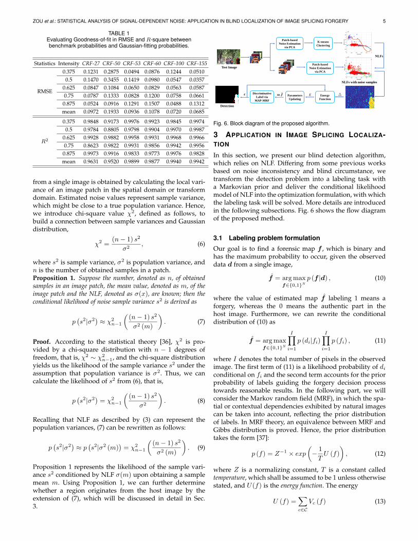
TABLE 1Evaluating Goodness-of-fit in RMSE and R-square betweenbenchmark probabilities and Gaussian-fitting probabilities.

Statistics Intensity CRF-27 CRF-50 CRF-53 CRF-60 CRF-100 CRF-155

RMSE

0.375 0.1231 0.2875 0.0494 0.0876 0.1244 0.05100.5 0.1470 0.3455 0.1419 0.0980 0.0547 0.0357

0.625 0.0847 0.1084 0.0650 0.0829 0.0563 0.05870.75 0.0787 0.1333 0.0828 0.1200 0.0758 0.06610.875 0.0524 0.0916 0.1291 0.1507 0.0488 0.1312mean 0.0972 0.1933 0.0936 0.1078 0.0720 0.0685

R2

0.375 0.9848 0.9173 0.9976 0.9923 0.9845 0.99740.5 0.9784 0.8805 0.9798 0.9904 0.9970 0.9987

0.625 0.9928 0.9882 0.9958 0.9931 0.9968 0.99660.75 0.8623 0.9822 0.9931 0.9856 0.9942 0.99560.875 0.9973 0.9916 0.9833 0.9773 0.9976 0.9828mean 0.9631 0.9520 0.9899 0.9877 0.9940 0.9942

from a single image is obtained by calculating the local vari-ance of an image patch in the spatial domain or transformdomain. Estimated noise values represent sample variance,which might be close to a true population variance. Hence,we introduce chi-square value χ2, defined as follows, tobuild a connection between sample variances and Gaussiandistribution,

χ2 =(n− 1) s2

σ2, (6)

where s2 is sample variance, σ2 is population variance, andn is the number of obtained samples in a patch.Proposition 1. Suppose the number, denoted as n, of obtainedsamples in an image patch, the mean value, denoted as m, of theimage patch and the NLF, denoted as σ(x), are known; then theconditional likelihood of noise sample variance s2 is derived as

p(s2|σ2

)≈ χ2

n−1

((n− 1) s2

σ2 (m)

). (7)

Proof. According to the statistical theory [36], χ2 is pro-vided by a chi-square distribution with n − 1 degrees offreedom, that is, χ2 ∼ χ2

n−1, and the chi-square distributionyields us the likelihood of the sample variance s2 under theassumption that population variance is σ2. Thus, we cancalculate the likelihood of s2 from (6), that is,

p(s2|σ2

)= χ2

n−1

((n− 1) s2

σ2

). (8)

Recalling that NLF as described by (3) can represent thepopulation variances, (7) can be rewritten as follows:

p(s2|σ2

)≈ p

(s2|σ2 (m)

)= χ2

n−1

((n− 1) s2

σ2 (m)

). (9)

Proposition 1 represents the likelihood of the sample vari-ance s2 conditioned by NLF σ(m) upon obtaining a samplemean m. Using Proposition 1, we can further determinewhether a region originates from the host image by theextension of (7), which will be discussed in detail in Sec.3.

Patch-based

Noise Estimation

via PCA

K-means

Clustering

Patch-based

Noise Estimation

via PCA

Discriminative

Label via

MAP-MRF

NLFs

NLFs with noise samples

Energy

Function

Parameters

Updating

𝝐 𝝎, 𝒇 E 𝒥𝑐

Test Image

Detection

Fig. 6. Block diagram of the proposed algorithm.

3 APPLICATION IN IMAGE SPLICING LOCALIZA-TION

In this section, we present our blind detection algorithm,which relies on NLF. Differing from some previous worksbased on noise inconsistency and blind circumstance, wetransform the detection problem into a labeling task witha Markovian prior and deliver the conditional likelihoodmodel of NLF into the optimization formulation, with whichthe labeling task will be solved. More details are introducedin the following subsections. Fig. 6 shows the flow diagramof the proposed method.

3.1 Labeling problem formulation

Our goal is to find a forensic map f , which is binary andhas the maximum probability to occur, given the observeddata d from a single image,

f = arg maxf∈0,1N

p (f |d) , (10)

where the value of estimated map f labeling 1 means aforgery, whereas the 0 means the authentic part in thehost image. Furthermore, we can rewrite the conditionaldistribution of (10) as

f = arg maxf∈0,1N

I∏i=1

p (di|fi)I∏i=1

p (fi) , (11)

where I denotes the total number of pixels in the observedimage. The first term of (11) is a likelihood probability of diconditional on fi and the second term accounts for the priorprobability of labels guiding the forgery decision processtowards reasonable results. In the following part, we willconsider the Markov random field (MRF), in which the spa-tial or contextual dependencies exhibited by natural imagescan be taken into account, reflecting the prior distributionof labels. In MRF theory, an equivalence between MRF andGibbs distribution is proved. Hence, the prior distributiontakes the form [37]:

p (f) = Z−1 × exp(− 1

TU (f)

), (12)

where Z is a normalizing constant, T is a constant calledtemperature, which shall be assumed to be 1 unless otherwisestated, and U(f) is the energy function. The energy

U (f) =∑c∈C

Vc (f) (13)

6

is a sum of clique potentials Vc(f) over all possible cliquesC. The value of Vc(f) depends on the local configurationof clique c. A clique c for (S,N ) is defined as a subset ofsites in S , where S contains the nodes i, and N determinesthe links between the nodes according to the neighboringrelationship. Considering the collection C of all cliques for(S,N ), (13) can be expanded as the sum of several terms asfollows:

U (f) =∑i∈C1

V1 (fi) +∑

i,i′∈C2

V2 (fi, fi′)

+∑

i,i′,i′′∈C3

V3 (fi, fi′ , fi′′) + · · · .(14)

In most cases, contextual constraints on both labels arewidely used because of their simple form and low cost incomputation, and they are encoded in the Gibbs energy aspair-site clique potentials. With clique potentials of up to 2sites, the energy takes the form

U (f) =∑i∈S

V1 (fi) +∑i∈S

∑i′∈N

V2 (fi, fi′) , (15)

where “∑i∈S” is equivalent to “

∑i∈C1” and

“∑i∈S

∑i′∈N ” equivalent to “

∑i,i′∈C2”. A particular

MRF can be specified by properly selecting V1 and V2. Forsingle-site cliques, the clique potentials depend on the labelas

V1 (fi) = α, if fi = 1, (16)

where α is the penalty against tampered authenticationunits. The higher α is, the fewer pixels will be assigned avalue of 1. This outcome has the effect of controlling thepercentage of sites labeled 1. As for pairwise contextualconstraints, it assumes that physical properties in a neigh-borhood of space present some coherence and generally donot change abruptly. In a simple case, the pair-site cliquepotentials can be defined as

V2 (fi, fi′) = g (fi − fi′) , (17)

where g (fi − fi′) is a function penalizing the violation ofsmoothness caused by the difference fi−fi′ . Here, we resortto a function taking the form

g (fi − fi′) = βi,i′ |fi − fi′ | , (18)

where βi,i′ is the penalty against nonequal labels on two-sitecliques. This value can be calculated as follows [29]:

βi,i′ = β0 + β1e− 1

2φ−2‖di,di′‖

22 , (19)

where ‖di, di′‖22 denotes L2 distance between two pixels(computed from RGB vectors). The first term encodes adefault, content-dependent penalty. The second term rep-resents the interactions of neighboring authentication units,with similarity attenuation controlled by parameter φ (em-pirically chosen to be 25). Thus, (18) guides a preferencetowards piecewise-constant- and contextual-dependency-based solutions.

Hence, we can rewrite (11) by taking the negative logand combining all the prior models above, as follows:

f = arg minf∈0,1N

I∑i=1

−log p (di|fi) + α∑i∈S

fi

+βi,i′∑i∈S

∑i′∈N

|fi − fi′ |.

(20)

The second and third terms are the penalty terms and havebeen discussed above. The first term (referred to as thelikelihood energy) depends only on the data.

3.2 Image tamper probability derivation

Since log p (di|fi) in (20) is a likelihood of observation diconditioned on label fi, we will discuss here how the imagetamper probability mixed with a different label fi deter-mines the likelihood energy. When a tamper probability Ptifor a patch is acquired, the label fi assigned to it should beconsistent with the requirement of optimization (20). Thatis, the wrong label leads to maximum likelihood energy,and the right one leads to minimum energy. Based on thisprinciple, we simply apply the following equation:

log p (d|f) =

log (1− Pti) , forf = 0,

log Pti , forf = 1.(21)

A smaller Pti indicates an authentic observation, and if f =1, which means a wrong inferred label, the log p (di|fi) willbe small while energy is opposite due to its taking a negativevalue in (20); and vice versa.

Assuming that two different NLFs have previously beenobtained precisely from an image, we are ready to derivethe tamper probability. Let one NLF, referred to as σ0,corresponds to the pristine, and the other NLF, referred toas σ1, corresponds to tampering. Hence, the likelihood oftampering can be derived, according to Bayes’ theorem andthe law of total probability [38], as follows:

Pt = p(s2 ∈ σ1 (m) |s2

)=

p(s2|s2 ∈ σ1 (m)

)p(s2 ∈ σ1 (m)

)∑1k=0 p (s2|s2 ∈ σk (m)) p (s2 ∈ σk (m))

,(22)

where p(s2|s2 ∈ σ1 (m)

)can be easily calculated by (8), and

p(s2 ∈ σ1 (m)

)takes the form:

p(s2 ∈ σ1 (m)

)=

∑i p(s2i |s2

i ∈ σ1 (m))∑1

k=0

∑i p (s2

i |s2i ∈ σ1 (m))

. (23)

Note that (22) is accurate when the assumption that twoNLFs can be obtained precisely is satisfied. Generally, anNLF is constructed by the sample variances in an image,and its precision depends on the number and estimationaccuracy of noise samples. The former is determined by theimage itself, while the latter depends on different methods.

3.3 Construction of NLFs in a tampered image

As the estimation of NLF is not our main work, we havefollowed [15] to construct the NLF. However, because theestimation of noise in [15] is slightly overestimated, wehave resorted to a PCA-based method [6] to estimate noisevariances.


First, the test image is decomposed into N non-overlappingB×B patches. Next, we estimate noise variances2n in every single patch by a PCA-based method. Mean-

while, the mean value mn of every patch is calculated asthe noise-free intensity. Then, we preliminarily and simplylocate several suspicious regions, according to the numer-ical differences only of noise variances, by running the K-means clustering algorithm. Consequently, a noise sampleset (mn, sn) is decomposed into two sets,

(m

[0]n , s

[0]n

)and

(m

[1]n , s

[1]n

), in which superscripts 0 and 1 represent

the original and suspicious regions, respectively. After ob-taining the noise sample set

(m

[i]n , s

[i]n

), a Bayesian MAP

inference is exploited to construct NLF σ[i], as follows:

xl = arg minxl

∑n

[−log Φ

(√kn

s[i]n

(s[i]n − eTnxTl − σ[i]

(m[i]n

)))

+

(eTnx

Tl + σ[i]

(m

[i]n

)− s[i]

n

)2

2(s

[i]n /√kn)2

+ xTl Λ−1xl,

(24)subject to

σ[i] = σ[i] + Exl ≥ 0. (25)

In the above formula, kn denotes the number of pixels ina patch; the matrix E = [ω1, · · · , ωm] ∈ Rd×m, where d =256, contains the principal components; en is the n-th rowof E; and Λ = diag(v1, · · · , vm) is the diagonal eigenvaluematrix whose elements correspond to principal componentsωm after PCA.

Note that all the samples involved in the constructionof NLF originate from smooth or flat patches. By doing so,some overestimated sample variances can be avoided thatwould otherwise affect NLF.

3.4 Combination strategy for refinement of tamperprobability

Recall from Sec. 3.2 that (22) regarding tamper probabilityis accurate when the assumption that two NLFs can beobtained precisely is strictly held. Generally, the pristineregion of a tampered image represents the majority andthe noise sample size in this region is also large enough,which is likely to result in an accurate NLF. However, whenthe size of the tampered region is quite small, the noisesample size will also consequently be small, which maydirectly lead to an inaccurate NLF estimation originatingfrom the tampered region. In the following dicussion, weare ready to study the strategy of refining inaccuracies intamper probability.

Considering that NLF estimated from the original area isrelatively accurate, we regard it as a benchmark. Note thatoriginal area here is an area initially taken as pristine, andit is generally credible even if some of noise from the patchin the original area are overestimated or a few tamperedregions are initially mistaken as the original. Inspiring bythe distance-based method for tampered detection [25], wecalculate the tampered probability as

Pt = 1− e−ζ‖si−σ[0](mi)‖

2 , (26)

where ζ is a difference-expanding operator (empirically cho-sen as 50), si denotes noise variances from aB/2×B/2 sizedpatch in an image, and σ[0] (mi) signifies the benchmarkNLF value of the sample mean mi. Thus, (26) indicatesthe distance between the estimated noise sample and ref-erence NLF representing the authentic baseline. The closerthe noise sample is to the reference curve, the less theprobability is. In other words, the region where the samplecomes from is more likely to be authentic. Note that weare calculating the noise variance in a smaller patch with asize of B/2×B/2, and applying them to (22) and (26). Thepurpose is to obtain more samples and make classificationsofter.

Now we face the problem of how to choose the properlikelihood. On the one hand, when the size of the tamperedregion is small, then we will have enough samples to con-struct the benchmark NLF, by which the likelihood based onthe benchmark curve will be relatively reliable. On the otherhand, if the size of the tampered region is large enough,(22) for tamper probability may yield better results. Here,we make a tradeoff to create a combination, resorting to a“steep” logistic function of shifted coordinates, as follows:

βp =1

1 + e−λ(Ar−δ), (27)

where βp is a coefficient assigned to the interaction likeli-hood to determine the percentage in the combination, Ardenotes the size of the tampered region, λ is the strength ofthe steepness, and δ represents how much the coordinatesshift. Consequently, we can compute the combination Jc as

Jc = (1− βp)J1 + βpJ2, (28)

where J1 denotes the likelihood based on the benchmarkcurve, as listed in (26), and J2 indicates the likelihoodbased on (22). For further reference, Appendix A providesa concrete numerical analysis between two probabilities J1

and J2.

3.5 Parameter estimation with a self-iterative strategyin MAP-MRF

Recalling the formulation of (20), we have three unknownparameters ω = α, β0, β1, which are vital for the finalsolution in MRF framework. Traditionally, the selection ofparameters is a supervised training process on the fullylabeled training image examples. Such an operation relies onthe assumption that a large number of images is available,which are known to the tampered region of interest. How-ever, in a blind scenario, we can only assume that we havea certain number of images, whose origin is unknown. In-spired by [12], we will use an iterative alternating algorithmto estimate the parameters. The algorithm iterates betweentwo steps: parameter estimation (looking for optimal ω) andinference (looking for optimal f based on estimated ω ofthe current step). Hence, we will formulate the estimationproblem in an energy minimization framework as(

f , ω)

= arg minf ,ω

E (Jc,ω,f) , (29)

where the energy function is equivalent to the right-handside of (20). Algorithm I presents a detailed demonstration.

8

Algorithm 1 Parameter estimation using an iterative alter-nating algorithmInput: The combination of likelihoods Jc and the maxi-

mum iteration Iter maxOutput: ω = α, β0, β1 and final decision label f

1: Initialize the label f approximately by K-means method.

2: repeat3: Minimize the energy E with fixed input label f to

estimate the ω with ω = arg minω E.4: Update ω: ω ← ω.5: Fix the MRF parameter ω and minimize the energy E

according to f = arg minf E.6: Update f : f ← f .7: until E converges or Iter max reached.

We will construct MRF using the UGM toolbox [39] forundirected graphical models and a max-flow algorithm forfaster GraphCuts [40]. Owing to higher accuracy and betterconvergence of LBP inference in the UGM toolbox, we haveobserved that most test cases converged before reachingmaximum iteration Iter max (we set it at 5 for rapidity).Even some cases reach the Iter max without convergence,the final decision f can also offer relatively good accuracy.Note the above inference process is completely unsuper-vised and no training sets is necessary. Given a new testimage, the optimal parameters and the inferred labels areestimated.

The complete implementation of the forgery localizationis presented in Algorithm II.

4 EXPERIMENTAL RESULTS ON SPLICING LOCA-TION ALGORITHM

In this section, we present experiments conducted on splic-ing tampered images to test our algorithm. In Sec. 4.1, weintroduce the experimental preparation, including imagedatasets and evaluation criterion. In Sec. 4.2, we carry outsome preliminary analysis to assess the performance of SDNin forgery localization. In Sec. 4.3, we evaluate our methodin quantitative and qualitative terms and then compareresults with some noise-related algorithms. Finally, in Sec.4.4, we measure the impact of lossy JPEG compression andscaling attack on images.

4.1 Experimental SetupIn order to assess the performance of forgery localization indifferent scenarios, we used five datasets, listed in Table 2together with their main features. The Columbia dataset [41]comprised forged images with splicing, but they were edge-salient and not realistic enough. Similar to the Columbiadataset, the UM-IPPR dataset [42] contained forged imageswith splicing objects by some simple manipulations. Themanipulations in the DSO-1 dataset [43], where imageswere saved in uncompressed PNG format, were carried outwith great care, and most of them were realistic. Forgeriesof various types were present in the Realistic TamperingDataset (RTD) proposed by Korus in [29]. The manipu-lated images, all uncompressed, appear extremely realistic,

Algorithm 2 The coefficients estimation with respect to theNLF from a single imageInput: Splicing tampered image yOutput: Decision map of forgery localization f

1: Decompose the input image y into N non-overlappingblocks with a size of B ×B.

2: Estimate the noise variance in each block us-ing PCA-based method, and noise sample set(mn, sn) |n ∈ 1, 2, · · · , N is obtained.

3: Use K-means clustering algorithm to preliminarily andsimply decompose noise sample set into

(m

[0]n , s

[0]n

)and

(m

[1]n , s

[1]n

).

4: Select noise samples originated from smooth blocks toconstruct the NLFs, σ[0] and σ[1], by using (24).

5: Decompose the input image y into 4N non-overlappingblocks with a size of B/2×B/2.

6: Estimate the noise variance in each new de-composed block using PCA-based method, with(mn, sn) |n ∈ 1, 2, · · · , 4N obtained.

7: Calculating the image tampered probabilities J1 and J2

by using (22) and (26).8: Combine two probabilities as JC by using (28) for

refinement.9: Estimate the MRF parameters

(f , ω

)by solving the

energy minimization problem (29) according to iterativealternating strategy.

10: Infer the decision map of forgery localization f bysolving the MAP-MRF optimization problem (20).

TABLE 2Datasets

Dataset Ref. # Camera Image Size formatColumbia [41] 4 757× 568− 1152× 768 TIF

USST-SPLC self-created 13 1920× 1080− 8368× 5584 TIFDSO-1 [43] unknown 2048× 1536 PNG

RTD (Korus) [29] 4 1920× 1080 TIFUM-IPPR [42] unknown 1152×768 JPG

although only a small number of cameras were involved.Notably, in our experiment, we only chose the forged imageswith splicing manipulation in the RTD for the target forsplicing forgery localization. The USST-SPLC dataset1 wasa self-created dataset containing 56 different tampered im-ages, which were created from authentic ones with differentISO settings using Adobe Photoshop, to approximate therealistic scenario. The tampered region could originate fromthe same camera with the host image or a different one.All the source pictures were downloaded from the famouscamera review website depeview.com.

For reference methods, we only considered noise-relatedmethods, listed as NOI1 [19], NOI2 [20], NOI4 [22],NOI-Multiscale [23], NOI-SVD [26], Splicebuster [27], andNoiseprint [33]. NOI1 and NOI2 were based on error levelanalysis and dependent on the noise intensity only. NOI4and NOI-SVD used the noise estimated in the PCA domainand SVD domain separately to reveal the noise incon-

1. https://1drv.ms/u/s!ArHfoaqCoSuIgkKpV9voJuFztoSv?e=HFQpfx


sistency in forged images. NOI-Multiscale was a methodof adopting the multiscale strategy and distance probabil-ity map to cluster the original and tampered region. InSplicebuster, the high-pass noise residual of the image wasemployed to extract rich features, and then these featureswere clustered using the EM algorithm to reveal possibleanomalies. In comparison, Noiseprint was a CNN-basedmethod to detect the traces of camera artifacts.

To evaluate the performance of SDN and the proposedalgorithm in forgery localization, we used precision, recall, ac-curacy, and F-score as assessment criteria, which are definedas follows:

precision =TP

TP + FP, (30)

recall =TP

TP + FN, (31)

accuracy =TP + TN

TP + TN + FP + FN, (32)

F =2× precision× recallprecision+ recall

, (33)

where TP, TN, FP, and FN denote the statistics of theobserved true positives, true negatives, false positives, andfalse negatives, respectively.

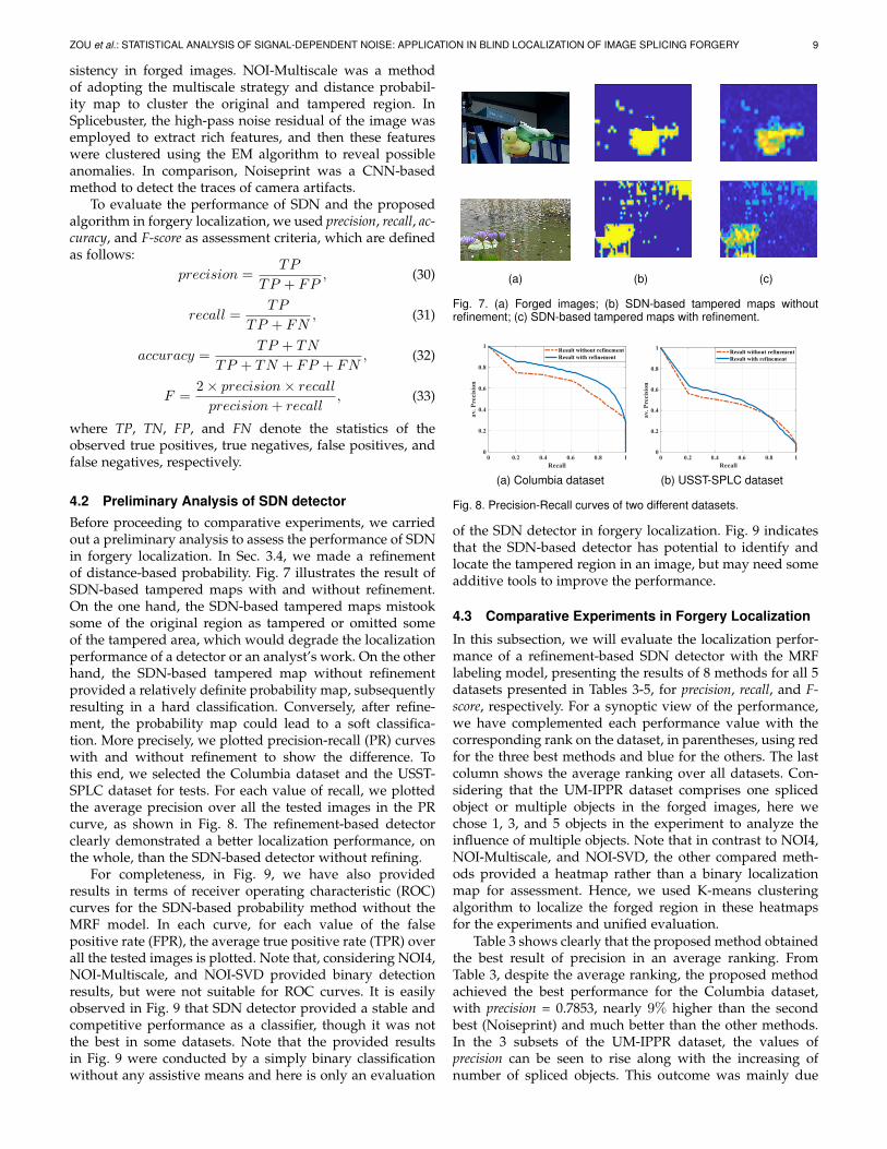
4.2 Preliminary Analysis of SDN detectorBefore proceeding to comparative experiments, we carriedout a preliminary analysis to assess the performance of SDNin forgery localization. In Sec. 3.4, we made a refinementof distance-based probability. Fig. 7 illustrates the result ofSDN-based tampered maps with and without refinement.On the one hand, the SDN-based tampered maps mistooksome of the original region as tampered or omitted someof the tampered area, which would degrade the localizationperformance of a detector or an analyst’s work. On the otherhand, the SDN-based tampered map without refinementprovided a relatively definite probability map, subsequentlyresulting in a hard classification. Conversely, after refine-ment, the probability map could lead to a soft classifica-tion. More precisely, we plotted precision-recall (PR) curveswith and without refinement to show the difference. Tothis end, we selected the Columbia dataset and the USST-SPLC dataset for tests. For each value of recall, we plottedthe average precision over all the tested images in the PRcurve, as shown in Fig. 8. The refinement-based detectorclearly demonstrated a better localization performance, onthe whole, than the SDN-based detector without refining.

For completeness, in Fig. 9, we have also providedresults in terms of receiver operating characteristic (ROC)curves for the SDN-based probability method without theMRF model. In each curve, for each value of the falsepositive rate (FPR), the average true positive rate (TPR) overall the tested images is plotted. Note that, considering NOI4,NOI-Multiscale, and NOI-SVD provided binary detectionresults, but were not suitable for ROC curves. It is easilyobserved in Fig. 9 that SDN detector provided a stable andcompetitive performance as a classifier, though it was notthe best in some datasets. Note that the provided resultsin Fig. 9 were conducted by a simply binary classificationwithout any assistive means and here is only an evaluation

(a) (b) (c)

Fig. 7. (a) Forged images; (b) SDN-based tampered maps withoutrefinement; (c) SDN-based tampered maps with refinement.

(a) Columbia dataset

(b) USST-SPLC dataset

Fig. 8. Precision-Recall curves of two different datasets.

of the SDN detector in forgery localization. Fig. 9 indicatesthat the SDN-based detector has potential to identify andlocate the tampered region in an image, but may need someadditive tools to improve the performance.

4.3 Comparative Experiments in Forgery Localization

In this subsection, we will evaluate the localization perfor-mance of a refinement-based SDN detector with the MRFlabeling model, presenting the results of 8 methods for all 5datasets presented in Tables 3-5, for precision, recall, and F-score, respectively. For a synoptic view of the performance,we have complemented each performance value with thecorresponding rank on the dataset, in parentheses, using redfor the three best methods and blue for the others. The lastcolumn shows the average ranking over all datasets. Con-sidering that the UM-IPPR dataset comprises one splicedobject or multiple objects in the forged images, here wechose 1, 3, and 5 objects in the experiment to analyze theinfluence of multiple objects. Note that in contrast to NOI4,NOI-Multiscale, and NOI-SVD, the other compared meth-ods provided a heatmap rather than a binary localizationmap for assessment. Hence, we used K-means clusteringalgorithm to localize the forged region in these heatmapsfor the experiments and unified evaluation.

Table 3 shows clearly that the proposed method obtainedthe best result of precision in an average ranking. FromTable 3, despite the average ranking, the proposed methodachieved the best performance for the Columbia dataset,with precision = 0.7853, nearly 9% higher than the secondbest (Noiseprint) and much better than the other methods.In the 3 subsets of the UM-IPPR dataset, the values ofprecision can be seen to rise along with the increasing ofnumber of spliced objects. This outcome was mainly due

10

(a) Columbia dataset

(b) DSO-1

(c) RTD (Korus)

(d) USST-SPLC

(e) UM-IPPR-1

(f) UM-IPPR-3

(g) UM-IPPR-5

Fig. 9. ROC curves of SDN detector for all datasets.

TABLE 3Experimental Results: Precision

Dataset Columbia USST-SPLC DSO-1 RTD (Korus) UM-IPPR-1 UM-IPPR-3 UM-IPPR-5 Av. RankProposed 0.7853(1) 0.5597(3) 0.3704(3) 0.2302(3) 0.6496(3) 0.8059(3) 0.8457(3) 2.7(1)

NOI1 0.5263(5) 0.2034(7) 0.1307(7) 0.1770(8) 0.6191(4) 0.9627(1) 0.9702(1) 4.7(6)NOI2 0.4451(7) 0.2158(6) 0.1873(6) 0.1340(7) 0.2607(8) 0.4038(8) 0.4952(6) 6.9(8)NOI4 0.6732(4) 0.3022(4) 0.1243(8) 0.1010(6) 0.5977(5) 0.9456(2) 0.9612(2) 4.4(5)

NOI-Multiscale 0.4293(8) 0.1396(8) 0.2147(4) 0.1169(4) 0.3107(7) 0.4805(6) 0.5360(5) 6.0(7)NOI-SVD 0.4832(6) 0.2932(5) 0.2069(5) 0.1062(5) 0.7529(1) 0.7989(4) 0.7773(4) 4.3(4)

Splicebuster 0.6934(3) 0.5885(1) 0.6197(2) 0.3639(1) 0.7154(2) 0.4596(7) 0.2003(8) 3.4(2)Noiseprint 0.6989(2) 0.5719(2) 0.7534(1) 0.3418(2) 0.5769(6) 0.5181(5) 0.3961(7) 3.6(3)

TABLE 4Experimental Results: Recall


NOI1 0.3963(4) 0.4671(7) 0.2039(7) 0.3710(6) 0.7807(3) 0.8895(1) 0.8680(1) 4.1(4)NOI2 0.2750(7) 0.4819(6) 0.1064(8) 0.1333(8) 0.3104(7) 0.3002(8) 0.2808(6) 7.1(8)NOI4 0.5778(3) 0.6351(3) 0.2060(6) 0.3659(7) 0.6314(6) 0.7057(4) 0.6701(5) 4.9(6)



to the fact that more spliced objects were beneficial forrecovering NLF of an alien region. Meanwhile, it is worthnoting that the proposed method did not always providethe best performance in terms of precision. For example, inthe USST-SPLC, DSO-1, and RTD datasets, the proposedmethod ranked third, after Splicebuster and Noiseprint.In fact, the USST-SPLC, DSO-1, and RTD datasets weremore complicated and realistic than the Columbia dataset.Accordingly, NLF inconsistence may be small, which affectsthe performance of the SDN-based detector. Nevertheless,the proposed method performed much better than the othernoise-related methods, which yielded at least 10% lower re-sults than the proposed method. Another specific case is thatSplicebuster and Noiseprint showed a dramatic impairmentin the UM-IPPR datasets; for example, Splicebuster ranked

only seventh, and Noiseprint ranked fifth in the UM-IPPR-3 dataset. Moreover, their performances degraded with anincreasing number of spliced objects. One reason might bethat the noise in the alien region of the UM-IPPR datasetwas added artificially and obeyed Gaussian distributiononly. The performance of Splicebuster and Noiseprint heresuggests that they fitted the real tampered scene well butperformances were limited to scenes where noise was addedmanually. However, the proposed method consistently pro-vided a satisfactory performance across all the datasets.

Tables 4 and 5 report the experimental results for therecall and F-score metrics. Like Table 3, the proposed methodaveragely ranked first in both the recall and F-score metrics.In Table 4, under the criterion of recall, we achieved abetter rank across the datasets for real noise, with the first


TABLE 5Experimental Results: F-score


NOI1 0.4521(5) 0.2834(7) 0.1593(6) 0.2397(4) 0.6906(3) 0.9247(1) 0.9163(1) 3.9(3)NOI2 0.3400(7) 0.2981(6) 0.1357(8) 0.1336(8) 0.2834(8) 0.3444(8) 0.3584(6) 7.3(8)NOI4 0.6219(3) 0.4095(4) 0.1550(7) 0.1583(7) 0.6141(5) 0.8082(3) 0.7896(3) 4.6(6)



ranking in the USST-SPLC dataset and the second ranking inthe DSO-1 and RTD datasets. Notably, Splicebuster, whichperformed well in terms of precision, showed a dramaticimpairment on the whole in the recall, meaning it tendedto omit some forgery in localization. Table 5 presents theresults of the F-score metric, which is a summarized qualityof precision and recall. It basically reflects the general resultsof precision and recall, shown in the Tables 3 and 4, with asmall change in relative ranking.

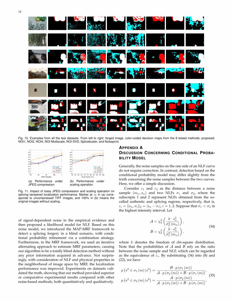
A better understanding of the actual quality of the resultscan be obtained by visually inspecting the examples in Fig.10. In this figure, color-coded decision maps display fourcolors: white, cyan, red, and black, where white denotesthe detected tampered region (TP), cyan indicates the de-tected authentic region (FP), red designates the undetectedtampered region (FN), and black signifies the undetectedauthentic region (TN). Notably, Fig. 10 demonstrates thatthe proposed refined SDN-based method with MRF modelachieved a better performance of localization though, itstill yielded some false positives. It is also worth notingthat Splicebuster and Noiseprint provided comparable lo-calization results in the datasets of real scenes but offeredrelatively poor performance in the UM-IPPR dataset, wherenoise was manually added in the spliced region. This resultalso validates the data in Tables 3-5.

4.4 Robustness Evaluation against Common Post-processing Operations

Considering that the spliced images might have undergonesome post-processing in network transmission, we studiedthe impact of these attacks on our proposed method, usingcomparisons with other noise-based algorithms. Due to thecommonplace of JPEG compression and scaling operationduring network transmission, lossy JPEG compression andscaling operation were applied to the Columbia datasetto test the robustness of the proposed splicing detectionmethod. The JPEG compression level was measured by thequality factor, a positive integer in the range of [1, 100]. Alarger quality factor means higher image quality (i.e., lesscompression), and vice versa. The scaling operation wasmeasured by a scale factor, which was within the intervalof (0, 1]; a scale factor of 1 meant the original image withoutany scaling. In this experiment, we created 4 new versionsof each image from the Columbia dataset with JPEG qualityfactors 85, 90, 95, and 100, and 5 new versions of each imagewith scale factors 50%, 65%, 75%, 85%, and 95%.

First, we evaluated the performance of our method foran attack by JPEG compression or scaling. Fig. 11 illustratesthe results, reflecting the criteria of recall, precision, accuracy,and F-score. In Fig. 11, it can be observed that all the criteriafor both types of attack decreased when the factors de-creased. However, the decreases in the two post-processingwere slightly different. In Fig. 11(a), when the JPEG qualityfactor decreased, precision and recall dramatically decreased,resulting in a decrease of the F-score. Accuracy was sus-tained when the quality factor was higher than 95, butdescended immediately and dramatically when the qualityfactor was lower than 95. Conversely, performance underthe scaling attack remained robust, to some extent, whenthe scaling factor was larger than 80, as presented in Fig.11(b). Moreover, it did not result in a downtrend like thatseen for JPEG compression, but presented a gradual andeven flat decline. For example, as shown in Fig. 11(b), withinthe interval of scaling factors [65%, 75%], the performanceof our algorithm remained consistent. On the whole, theproposed method was able to sustain robustness in thescaling operation when the scaling factor was within acertain range. In contrast, JPEG compression destroyed thenoise characteristic of an image, making it likely to degradethe performance of the proposed method.

Next, we compared our algorithm with other noise-inconsistent-based algorithms for localization performanceunder the attacks of lossy JPEG compression and scaling op-eration. Comparisons are exhibited in Figs. 12 and 13. Figs.12 and 13 reveal that the performances of all the methodsdecreased as the quality factor declined, and the proposedmethod with different quality factors provided superior orcomparative experimental results, especially when qualityfactors were high. Meanwhile, Fig. 13 clearly demonstratesthat our performance on scaling was little changed withinthe interval above the factor of 75% and between the factorsof 65% and 75% but decreased when the factor droppedfrom 75% to 65%. Note that in Figs. 12 and 13, accuraciesregarding both attacks for all methods are similar and con-sistent for different parameters. This outcome is mainly dueto the fact that the TN (corresponding to a pristine region ina tampered image) of detection was dominant.

5 CONCLUSION

This work proposed a novel algorithm for locating a splic-ing forgery in digital images by applying the likelihoodmodel of NLFs. We first analyzed the statistical model

12

Fig. 10. Examples from all the test datasets. From left to right: forged image, color-coded decision maps from the 8 tested methods: proposed,NOI1, NOI2, NOI4, NOI-Multiscale, NOI-SVD, Splicebuster, and Noiseprint.

(a) Performance underJPEG compression

(b) Performance underscaling operation

Fig. 11. Impact of lossy JPEG compression and scaling operation onsplicing tampered localization performance. Marker at ∞ in (a) corre-sponds to uncompressed TIFF images, and 100% in (b) means theoriginal images without scaling.

of signal-dependent noise in the empirical evidence andthen proposed a likelihood model for NLF. Based on thisnoise model, we introduced the MAP-MRF framework todetect a splicing forgery in a blind scenario, with condi-tional probability refinement via a combination strategy.Furthermore, in the MRF framework, we used an iterativealternating approach to estimate MRF parameters, causingour algorithm to be a totally blind detection method withoutany prior information acquired in advance. Not surpris-ingly, with consideration of NLF and physical properties inthe neighborhood of image space by MRF, the localizationperformance was improved. Experiments on datasets vali-dated the truth, showing that our method provided superioror comparative experimental results compared with othernoise-based methods, both quantitatively and qualitatively.

APPENDIX ADISCUSSION CONCERNING CONDITIONAL PROBA-BILITY MODEL

Generally, the noise samples on the one side of an NLF curvedo not require correction. In contrast, detection based on theconditional probability model may differ slightly from thetruth concerning the noise samples between the two curves.Here, we offer a simple discussion.

Consider ε1 and ε2 as the distance between a noisesample (mn, sn) and two NLFs σ1 and σ2, where thesubscripts 1 and 2 represent NLFs obtained from the so-called authentic and splicing regions, respectively, that is,εi = ‖sn, σi‖2 = |sn − σi|, i = 1, 2. Suppose that σ1 < σ2 inthe highest intensity interval. Let

A = χ2k

(k · s2

n

σ22 (mn)

),

B = χ2k

(k · s2

n

σ21 (mn)

),

(34)

where k denotes the freedom of chi-square distribution.Note that the probabilities of A and B rely on the ratiobetween the noise sample and NLF, which can be regardedas the equivalence of εi. By substituting (34) into (8) and(22), we have

p(s2 ∈ σ1 (m) |s2

)=

B · p (σ1 (m))

A · p (σ2 (m)) + B · p (σ1 (m)),

p(s2 ∈ σ2 (m) |s2

)=

A · p (σ2 (m))

A · p (σ2 (m)) + B · p (σ1 (m)),

(35)


(a) precision

(b) F-score

(c) recall

(d) accuracy

Fig. 12. Robustness comparisons on lossy JPEG compression.

(a) precision

(b) F-score

(c) recall

(d) accuracy

Fig. 13. Robustness comparisons on scaling operation.

where p (σi (m)) is the p(s2n ∈ σi (m)

)for short. First, we

will study the situation of the noise samples on the one sideof an NLF curve. With respect to the noise samples on theone side of the NLF σ1, (that is, these noise samples lie under

14

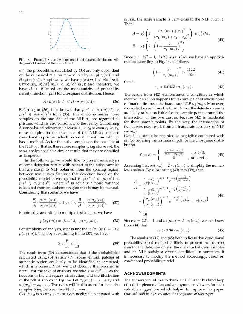
Fig. 14. Probability density function of chi-square distribution withdegrees of freedom at the k = 322 − 1.

σ1), the probabilities calculated by (35) are only dependenton the numerical relation represented by A · p(σ2(m)) andB · p(σ1(m)). Empirically, we have p(σ2(m)) < p(σ1(m)).Obviously, s2

n/σ22(mn) < s2

n/σ21(mn); and therefore, we

have A < B based on the monotonicity of probabilitydensity function (pdf) for chi-square distribution. Hence,

A · p (σ2 (m)) < B · p (σ1 (m)) . (36)

Referring to (36), it is known that p(s2 ∈ σ1(m)|s2) >p(s2 ∈ σ2(m)|s2) from (35). This outcome means noisesamples on the one side of the NLF σ1 are regarded aspristine, which is also consonant to the reality. Concerningdistance-based refinement, because ε1 < ε2 or even ε1 ε2,noise samples on the one side of the NLF σ1 are alsoconsidered as pristine, which is consistent with probability-based method. As for the noise samples on the one side ofthe NLF σ2, (that is, these noise samples lying above σ2), thesame analysis yields a similar result, that they are classifiedas tampered.

In the following, we would like to present an analysisof some detection results with respect to the noise samplesthat are closer to NLF obtained from the splicing region,between two curves. Suppose that detection based on theprobability model is wrong; that is, p(s2 ∈ σ1(m)|s2) <p(s2 ∈ σ2(m)|s2), where s2 is actually a noise variancecalculated from an authentic region that is may be textural.Considering this scenario, we have

BA· p (σ1 (m))

p (σ2 (m))< 1⇔ 0 <

BA<p (σ2 (m))

p (σ1 (m)). (37)

Empirically, according to multiple test images, we have

p (σ1 (m)) ≈ (8 ∼ 15) · p (σ2 (m)) . (38)

For simplicity of analysis, we assume that p (σ1 (m)) = 10×p (σ2 (m)). Then, by substituting it into (37), we have

0 <BA<

1

10. (39)

The result from (39) demonstrates that if the probabilitiescalculated using (34) satisfy (39), some textural patches ofauthentic region are likely to be identified as tampered,which is incorrect. Next, we will describe this scenario indetail. For the sake of analysis, we take k = 322 − 1 as thefreedom of the chi-square distribution, and the illustrationof the pdf is shown in Fig. 14. Let σ2(mn) = sn + ε2 andσ1(mn) = sn− ε1. Two cases will be discussed for the noisesamples lying between two NLF curves.Case 1: ε2 is so tiny as to be even negligible compared with

ε1, i.e., the noise sample is very close to the NLF σ2(mn).Then

A = χ2k

(k · (σ1 (mn) + ε1)

2

(σ1 (mn) + ε1 + ε2)2

)≈ χ2

k (k) ,

B = χ2k

(k ·(

1 +ε1

σ1 (mn)

)2).

(40)

Since k = 322 − 1, if (39) is satisfied, we have an approxi-mation according to Fig. 14, as follows:(

1 +ε1

σ1 (mn)

)2

>1122

1021, (41)

that is,ε1 > 0.0483 · σ1 (mn) . (42)

The result from (42) demonstrates a condition in whichincorrect detection happens for textural patches whose noiseestimation lies near the inaccurate NLF σ2(mn). Moreover,it can also be seen from the formula that the detection resultsare likely to be unreliable for the sample points around theintersection of the two curves, because (42) is incidentalfor these sample points. By the way, the intersection oftwo curves may result from an inaccurate recovery of NLFσ2(mn).Case 2: ε2 cannot be regarded as negligible compared withε1. Considering the formula of pdf for the chi-square distri-bution

f (x; k) =

xk/2−1e−x/2

2k/2−1Γ(k/2), x > 0,

0 , otherwise.(43)

Assuming that σ2(mn) = 2 · σ1(mn) to simplify the numer-ical analysis. By substituting (43) into (39), then

BA

=

(k·s2n

σ21(mn)

)k/2−1

e− 1

2

(k·s2n

σ21(mn)

)

(k·s2n

σ22(mn)

)k/2−1e− 1

2

(k·s2n

σ22(mn)

)

=

(σ2 (mn)

σ1 (mn)

)k−2

e− k·s

2n

2

(1

σ21(mn)− 1

σ22(mn)

)

<1

10.

(44)

Since k = 322 − 1 and σ2(mn) = 2 · σ1(mn), we can knowfrom (44) that

ε1 > 0.36 · σ1 (mn) . (45)

The results of (42) and (45) both indicate that conditionalprobability-based method is likely to present an incorrectclue for the detection only if the distance between samplesand an NLF satisfy a certain condition. In summary, itis necessary to modify the method accordingly, based onconditional probability model.

ACKNOWLEDGMENTS

The authors would like to thank Dr B. Liu for his kind helpof code implementation and anonymous reviewers for theirvaluable suggestions which helped to improve this paper.Our code will be released after the acceptance of this paper.


REFERENCES

[1] A. C. Bovik, Handbook of Image and Video Processing (Communica-tions, Networking and Multimedia). Orlando, FL: Academic Press,2005.

[2] L. Dong, J. Zhou, and Y.Y. Tang, “Noise level estimation fornatural images based on scale-invariant kurtosis and piecewisestationarity,” IEEE Trans. Image Process., vol. 26, no. 2, pp. 1017-1030, Feb. 2017.

[3] D. Zoran and Y. Weiss, “Scale invariance and noise in naturalimages,” in Proc. IEEE Int. Conf. Comput. Vis., pp. 2209–2216,Sep./Oct. 2009.

[4] C. Tang, X. Yang, and G. Zhai, “Noise estimation of natural imagesvia statistical analysis and noise injection,” IEEE Trans. CircuitsSyst. Video Technol., vol. 25, no. 8, pp. 1283-1294, Aug. 2015.

[5] B. Ma, J. Yao, Y. Le, C. Qin, H. Yao, “Efficient Image NoiseEstimation Based on Skewness Invariance and Adaptive NoiseInjection,” IET Image Process., vol. 14, no. 7, pp. 1393-1401, May2020.

[6] S. Pyatykh, J. Hesser, and L. Zheng, “Image noise level estimationby principal component analysis,” IEEE Trans. Image Process., vol.22, no. 2, pp. 687–699, Feb. 2013.

[7] C.-H. Wu and H.-H. Chang, “Superpixel-based image noise vari-ance estimation with local statistical assessment,” EURASIP Int. J.Image Video Process., vol. 2015, no. 1, pp. 1–12, Dec. 2015.

[8] A. Foi, M. Trimeche, V. Katkovnik, and K. Egiazarian, “PracticalPoissonian–Gaussian noise modeling and fitting for single-imageraw data,” IEEE Trans. Image Process., vol. 17, no. 10, pp. 1737–1754,Oct. 2008.

[9] L. Dong, J. Zhou, and Y.Y. Tang,” Effective and fast estimation forimage sensor noise via constrained weighted least squares,” IEEETrans. Image Process., vol. 27, no. 6, pp. 2715-2730, Jun. 2018.

[10] S. Lin, J. Gu, S. Yamazaki, and H.-Y. Shum, “Radiometric calibra-tion from a single image,” in Proc. IEEE Comput. Soc. Conf. Comput.Vis. Pattern Recognit., vol. 2, pp. 938–945, Jun. 2004.

[11] S. Lin and L. Zhang, “Determining the radiometric responsefunction from a single grayscale image,” in Proc. IEEE Comput. Soc.Conf. Comput. Vis. Pattern Recognit., vol. 2, pp. 66–73, Jun. 2005.

[12] J. Takamatsu, Y. Matsushita, and K. Ikeuchi, “Estimating cameraresponse functions using probabilistic intensity similarity,” inProc. IEEE Comput. Soc. Conf. Comput. Vis. Pattern Recognit.,pp. 1-8, Jun. 2008.

[13] Y. Tai, X. Chen, S. Kim, F. Li, J. Yang, J. Yu, Y. Matsushita,and M. Brown, “Nonlinear camera response functions and imagedeblurring: Theoretical analysis and practice,” IEEE Trans. PatternAnal. Mach. Intell., vol. 35, no. 10, pp. 2498-2512, Oct. 2013.

[14] C. Chen, S. McCloskey, and J. Yu, “Analyzing modern cameraresponse functions,” in Proc. IEEE Winter Conf. Appl. Comput.Vis., pp.1961-1969, Jan. 2019.

[15] C. Liu, R. Szeliski, S.B. Kang, C.L. Zitnick, and W.T. Freeman,“Automatic estimation and removal of noise from a single image,”IEEE Trans. Pattern Anal. Mach. Intell., vol. 30, no. 2, pp. 299-314,Feb. 2008.

[16] J. Yang, Z. Wu, and C. Hou, “Estimation of signal-dependentsensor noise via sparse representation of noise level functions,”in Proc. IEEE Int. Conf. Image Process., pp. 673–676, Sep./Oct. 2012.

[17] J. Yang, Z. Gan, Z. Wu, and C. Hou, “Estimation of signal-dependent noise level function in transform domain via a sparserecovery model,” IEEE Trans. Image Process., vol. 24, no. 5, pp.1561–1572, May 2015.

[18] T. H. Thai, F. Retraint and R. Cogranne, ”Generalized signal-dependent noise model and parameter estimation for naturalimages”, Signal Process., vol. 114, pp. 164-170, Sep. 2015.

[19] B. Mahdian and S. Saic, “Using noise inconsistencies for blindimage forensics,” Image and Vision Computing, vol. 27, no. 10, pp.1497–1503, 2009.

[20] S. Lyu, X. Pan, and X. Zhang, “Exposing region splicing forgerieswith blind local noise estimation,” Int. J. of Compt. Vis., vol. 110,no. 2, pp. 202–221, 2014.

[21] H. Yao, F. Cao, Z. Tang, J. Wang, and T. Qiao, “Expose noise levelinconsistency incorporating the inhomogeneity scoring strategy,”Multimedia Tools Appl., vol. 77, pp. 18139–18161, July 2018.

[22] H. Zeng, Y. Zhan, X. Kang, and X. Lin, “Image splicing localizationusing PCA-based noise level estimation,” Multimedia Tools Appl.,vol. 76, no. 4, pp. 4783–4799, Feb. 2017.

[23] C.-M. Pun, B. Liu, and X.-C. Yuan, “Multi-scale noise estimationfor image splicing forgery detection,” J. Vis. Commun. Image Repre-sent., vol. 38, pp. 195–206, Mar. 2016.

[24] H. Yao, S. Wang, X. Zhang, C. Qin, and J. Wang, “Detecting imagesplicing based on noise level inconsistency,” Multimedia ToolsAppl., vol. 76, no. 10, pp. 12457–12479, May 2017.

[25] N. Zhu and Z. li, “Blind image splicing detection via noise levelfunction,” Signal Process.: Image Commun., vol. 68, pp. 181-192,2018.

[26] B. Liu and C.-M. Pun, Locating splicing forgery by adaptive-SVDnoise estimation and vicinity noise descriptor, Neurocomputing,vol. 387, pp. 172-187, 2020.

[27] D. Cozzolino, G. Poggi, and L. Verdoliva, “Splicebuster: A newblind image splicing detector,” in IEEE International Workshop onInformation Forensics and Security, 2015, pp. 1–6.

[28] M. Chen, J. Fridrich, M. Goljan, and J. Lukas, “Determining imageorigin and integrity using sensor noise,” IEEE Trans. Inf. ForensicsSecurity, vol. 3, no. 4, pp. 74–90, 2008.

[29] P. Korus and J. Huang, “Multi-scale Analysis Strategies in PRNU-based Tampering Localization,” IEEE Trans. Inf. Forensics Security,vol. 12, no. 4, Apr, 2017.

[30] D. Cozzolino, F. Marra, G. Poggi, C. Sansone, and L.Verdoliva,“PRNU-based forgery localization in a blind scenario,”in International Conference on Image Analysis and Processing, 2017,pp. 569–579.

[31] M. Barni, L. Bondi, N. Bonettini, P. Bestagini, A. Costanzo, M.Maggini, B. Tondi, and S. Tubaro, “Aligned and non-aligneddouble JPEG detection using convolutional neural networks,” J.Vis. Commun. Image Represent., vol. 49, pp. 153–163, 2017.

[32] L. Bondi, S. Lameri, D. Guera, P. Bestagini, E. Delp, and S.Tubaro, “Tampering detection and localization through clusteringof camera-based CNN features,” in IEEE CVPR Workshops, 2017.

[33] D. Cozzolino and L. Verdoliva, “Noiseprint: A CNN-based cameramodel fingerprint,” IEEE Trans. Inf. Forensics Security, vol. 15, no.1, pp. 14–27, 2020.

[34] G. E. Healey and R. Kondepudy, “Radiometric CCD cameracalibration and noise estimation,” IEEE Trans. Pattern Anal. Mach.Intell., vol. 16, no. 3, pp. 267–276, Mar. 1994.

[35] M.D. Grossberg and S.K. Nayar, “Modeling the Space of CameraResponse Functions,” IEEE Trans. Pattern Anal. Mach. Intell., vol.26, no. 10, pp. 1272-1282, Oct. 2004.

[36] M. Evans, N. Hastings, and B. Peacock. Statistical Distributions. 2nded., Hoboken, NJ: John Wiley & Sons, Inc., 1993.

[37] S. Z. Li, Markov Random Field Modeling in Image Analysis. New York,NY, USA: Springer-Verlag, 2001.

[38] A. Papoulis. Probability, Random Variables, and Stochastic Processes,2nd ed. New York: McGraw-Hill, 1984.

[39] M. Schmidt. (2011). UGM: A MATLAB Toolbox forProbabilistic Undirected Graphical Models. [Online]. Available:http://www.cs.ubc.ca/∼schmidtm/Software/UGM.html

[40] Y. Boykov and V. Kolmogorov, “An Experimental Comparisonof Min-Cut/Max-Flow Algorithms for Energy Minimization inVision,” IEEE Trans. Pattern Anal. Mach. Intell., vol. 26, no. 9, pp.1124–1137, Sept. 2004.

[41] Y.-F. Hsu, S.-F. Chang, “Detecting Image Splicing Using GeometryInvariants and Camera Characteristics Consistency,” in Proc. IEEEInt. Conf. Multimedia Expo, Jul. 2006, pp. 549–552.

[42] Um-ippr splicing forgery database. [Online]. Available:https://www.dropbox.com/s/y0r6dzjjpbr49ak/UM-IPPR%20Splicing%20Forgery%20Database.7z?dl=0.

[43] T. J. de Carvalho, C. Riess, E. Angelopoulou, H. Pedrini, and A.Rocha, “Exposing digital image forgeries by illumination colorclassification,” IEEE Trans. Inf. Forensics Security, vol. 8, no. 7,pp. 1182–1194, Jul. 2013

Mian Zou received B.S. degree in electrical engineering from HefeiUniversity of Technology, China, in 2018. He is currently pursuing anM.S. degree in electrical engineering from University of Shanghai forScience and Technology, China. His research interests include imageprocessing and multimedia security.

http://www.cs.ubc.ca/~schmidtm/Software/UGM.html

16

Heng Yao received the B. Sc. degree from Hefei University of Technol-ogy, China, in 2004, the M. Eng. degree from Shanghai Normal Univer-sity, China, in 2008, and the Ph. D. degree in signal and information pro-cessing from Shanghai University, China, in 2012. Since 2012, he hasbeen with the faculty of the School of Optical-Electrical and ComputerEngineering, University of Shanghai for Science and Technology, wherehe is currently an Associate Professor. His research interests includemultimedia security, image processing, and pattern recognition. He hascontributed more than 40 international peer-reviewed journal papers.

Chuan Qin received the B.S. degree in electronic engineering and theM.S. degree in signal and information processing from the Hefei Univer-sity of Technology, Anhui, China, in 2002 and 2005, respectively, andthe Ph.D. degree in signal and information processing from ShanghaiUniversity, Shanghai, China, in 2008. Since 2008, he has been with theFaculty of the School of Optical-Electrical and Computer Engineering,University of Shanghai for Science and Technology, where he is cur-rently a Professor. He was with Feng Chia University, Taiwan, as a Post-Doctoral Researcher, from 2010 to 2012. His research interests includeimage processing and multimedia security. He has published over 130papers in these research areas.

Xinpeng Zhang received the B.S. degree in computational mathematicsfrom Jilin University, China, in 1995, and the M.E. and Ph.D. degreesin communication and information system from Shanghai University,China, in 2001 and 2004, respectively. Since 2004, he has been with theFaculty of the School of Communication and Information Engineering,Shanghai University, where he is currently a Professor. He was withthe State University of New York at Binghamton as a Visiting Scholarfrom 2010 to 2011 and with the Konstanz University as an Experi-enced Researcher small sponsored by the Alexander von HumboldtFoundation from 2011 to 2012. He is currently with the Faculty of theSchool of Computer Science, Fudan University. His research interestsinclude multimedia security, image processing, and digital forensics. Hehas published over 200 papers in these areas. He has served as anAssociate Editor for the IEEE Transactions on Information Forensics andSecurity from 2014 to 2017.

Date post:	22-Mar-2022
Category:	Documents
Upload:	others
View:	2 times
Download:	0 times

1 Statistical Analysis of Signal-Dependent Noise ...

Documents