1 Testing a Hypothesis about means The contents in this chapter are from Chapter 12 to Chapter 14 of...

1

Testing a Hypothesis about means

The contents in this chapter are from Chapter 12 to Chapter 14 of the textbook. Testing a single mean Testing two related means Testing two independent means

2

Testing a single mean

This chapter uses the gssft.sav data, which includes data for fulltime workers only.

The variables are: Hrsl: number of hours worked last week Agecat: age category Rincome: respondents income

3

Example The left plot is a

histogram of the number of hours worked in the previous week for 437 college graduates

The peak at 40 hours is higher than you would expect for a normal distribution.

There is also a tail toward larger values of hours worked.

It appears that people are more likely to work a long week than a short week.

4

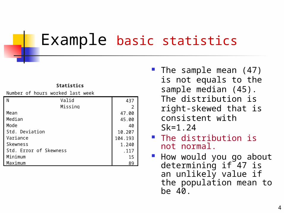
Example basic statistics

Statistics

Number of hours worked last week437

247.0045.00

4010.207

104.1931.240.117

1589

ValidMissing

N

MeanMedianModeStd. DeviationVarianceSkewnessStd. Error of SkewnessMinimumMaximum

The sample mean (47) is not equals to the sample median (45). The distribution is right-skewed that is consistent with Sk=1.24

The distribution is not normal.

How would you go about determining if 47 is an unlikely value if the population mean to be 40.

5


The variance is unknown, The statistic

The rejection region

The critical value of t can be found in many textbooks or SPSS.

s

μXnt 0

)2/(or )2/( 11 αttαtt nn

0100 H H :,:

6


The standard error of the mean is The t -statistic

The 95% confidence interval of the difference is

490437210 ./.

One-Sample Test

14.326 436 .000 6.995 6.04 7.96Number of hoursworked last week

t dfSig.

(2-tailed)Mean

Difference Lower Upper

95% ConfidenceInterval of the

Difference

Test Value = 40

31420710

4047427t .

.

967x046 ..

7

The t-distribution

The statistic used in the previous page follows a t-distribution with n-1 degrees of freedom.

This is a 2-tailed test. The p-value is the probability that a sample t value

is greater than 14.3 or less than -14.3. The p-value in this example is less than 0.0005. We can conclude that it’s quite unlikely that

college graduates work a 40-hour on average.

8

Normal approximation

The degree of freedoms in this test is 437-1=436. The t distribution is very close to the normal. The critical values or confidence interval can be determined based on the normal population.

99

The 95% confidence interval is given by

957047043046

427

2071096147

427

2071096147

s961x

s961x

.,.

..,

...,.

Descriptives

47.00 .48846.04

47.96

46.2345.00

104.19310.207

15897410

1.240 .1172.356 .233

MeanLower BoundUpper Bound

95% ConfidenceInterval for Mean

5% Trimmed MeanMedianVarianceStd. DeviationMinimumMaximumRangeInterquartile RangeSkewnessKurtosis

Number of hoursworked last week

Statistic Std. Error

10

Hypothesis Testing

The p-value is the probability of getting a test statistic equal to or more extreme than the sample result, given that the null hypothesis is true.

gomust H then low, is value- theIf

Hreject you , value- theIf

Hreject not doyou , value- theIf

0

0

0

p

αp

αp

11

Testing a Hypothesis about Two related means

We use the endoph.sav data set provided by the author.

Dale et al. (1987) investigated the possible role of in the collapse of runners.

are morphine ( 吗啡 )-like substances manufactured in the body.

They measured plasma ( 血浆 ) concentrations for 11 runners before and after they participated in a half-marathon run.

The question of interest was whether average

levels changed during a run.endorphins

endorphins

endorphinsendorphins

)( 内啡肽

12


Case Summariesa

4.30 29.60 25.304.60 25.10 20.505.20 15.50 10.305.20 29.60 24.406.60 24.10 17.507.20 37.80 30.608.40 20.20 11.809.00 21.90 12.90

10.40 14.20 3.8014.00 34.60 20.6017.80 46.20 28.40

11 11 11

1234567891011

NTotal

before after diff

Limited to first 100 cases.a.

13


This problem is recommended to use the paired-samples t test.

One-Sample Statistics

11 18.7364 8.32974 2.51151diffN Mean

Std.Deviation

Std. ErrorMean

One-Sample Test

7.460 10 .000 18.73636 13.1404 24.3324difft df

Sig.(2-tailed)

MeanDifference Lower Upper


Difference

Test Value = 0

14


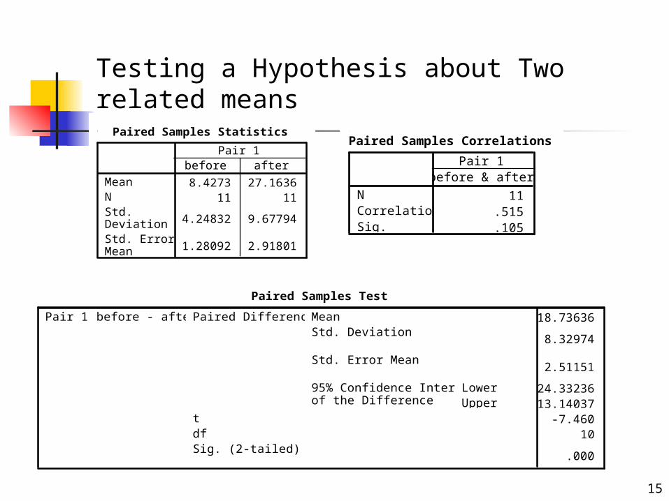
The average difference is 18.74 that is large comparing with S.D.=8.3.

The 95% confidence interval for the average difference is (13.14, 24.33) that does not includes the value of o, you can reject the hypothesis.

An equivalent way or testing the hypothesis is the t test. The p-value is less than 0.0005, we should reject the hypothesis.

15


Paired Samples Statistics

8.4273 27.163611 11

4.24832 9.67794

1.28092 2.91801

MeanNStd.DeviationStd. ErrorMean

before afterPair 1

Paired Samples Correlations

11.515.105

NCorrelationSig.

before & afterPair 1

Paired Samples Test

-18.73636

8.32974

2.51151

-24.33236-13.14037

-7.46010

.000

MeanStd. Deviation

Std. Error Mean

LowerUpper

95% Confidence Intervalof the Difference

Paired Differences

tdfSig. (2-tailed)

before - afterPair 1

16

diff Stem-and-Leaf Plot Frequency Stem & Leaf 1.00 0 . 3 4.00 1 . 0127 5.00 2 . 00458 1.00 3 . 0 Stem width: 10.00 Each leaf: 1 case (s)Each difference uses only the first two digits with

rounding.


17

All the differences are positive. That is, the after values are always greater than the before values.

The stem-and-leaf plot doesn’t suggest any obvious departures from normality.

A normal probability plot, or Q-Q plot, can helps us to test the normality of the data.


18

Normal Probability Plot

For each data point, the Q-Q plot shows the observed value and the value that is expected if the data are a sample from a normal distribution.

The points should cluster around a straight line if the data are from a normal distribution.

The normal Q-Q plot of the difference variable is nor or less linear, so the assumption of normality appears to be reasonable.

19

Normal Probability Plot

20

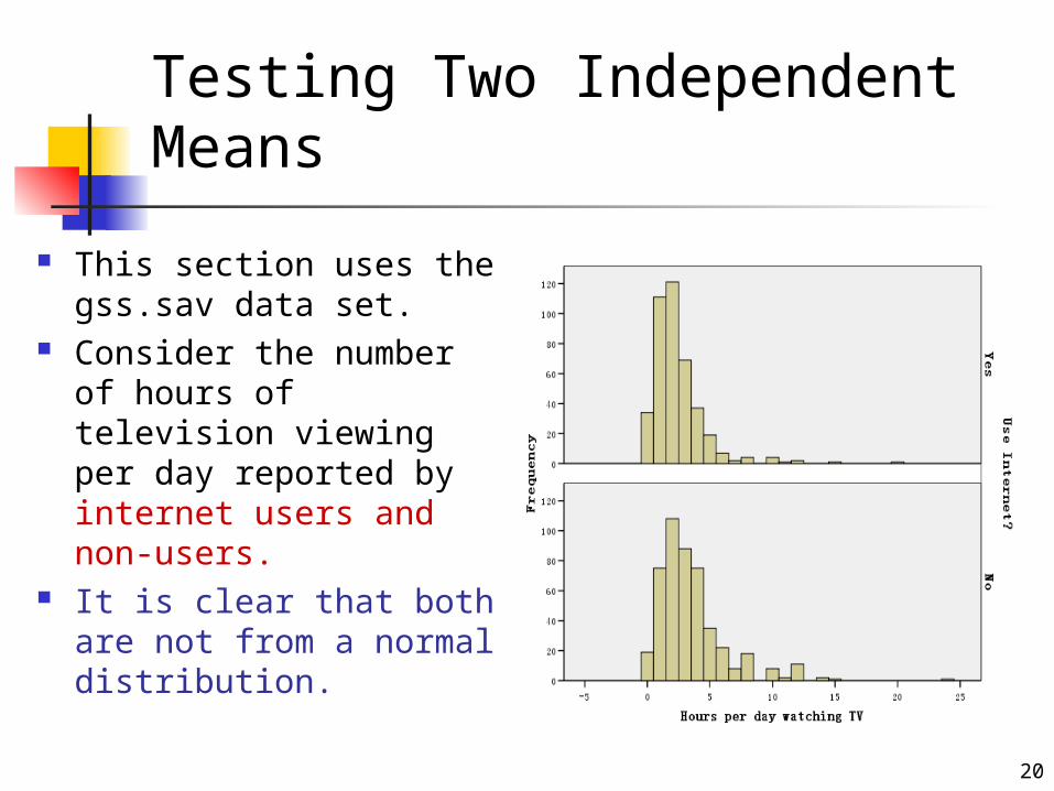
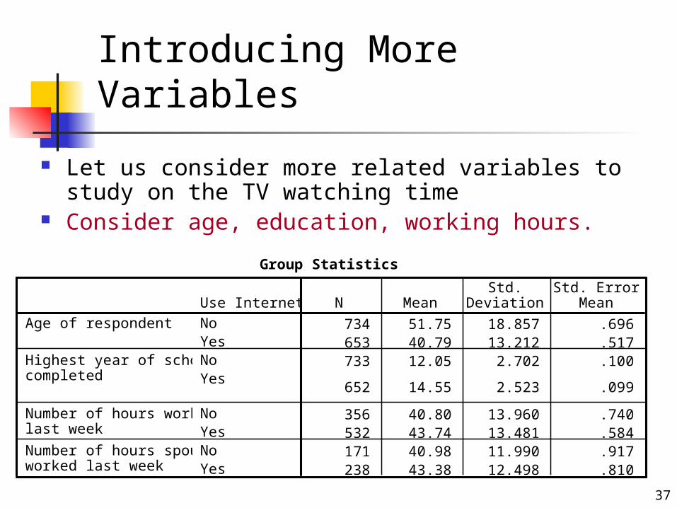
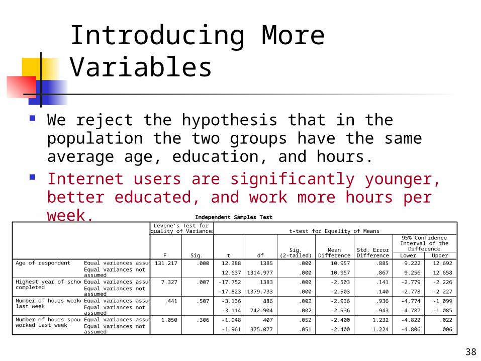
Testing Two Independent Means

This section uses the gss.sav data set.

Consider the number of hours of television viewing per day reported by internet users and non-users.

It is clear that both are not from a normal distribution.

21


We find that there are some problems in the data. There are people who report watching television

for 24 hours a day!! It is impossible. Watch TV is not a very well-defined term. If you

have the TV on while you are doing homework, are you studying or watching TV?

The observations in these two groups are independent. This fact implies “two independent means”.

22


Descriptives

3.52 2.423.26 2.22

3.77 2.63

3.22 2.183.00 2.00

7.801 4.6042.793 2.146

0 024 2024 202 2

2.164 3.0667.946 16.086.128 .106.112 .120.224 .240

MeanLower BoundUpper Bound

95% ConfidenceInterval for Mean

5% Trimmed MeanMedianVarianceStd. DeviationMinimumMaximumRangeInterquartile RangeSkewnessKurtosisMeanSkewnessKurtosis

Statistic

Std. Error

Hours per daywatching TV

No YesUse Internet?

23


Two sample means, 2.42 hours of TV viewing and 3.52 hours for those who don’t use the internet. A difference is about 1.1 hours.

The 5% trimmed means, which are calculated by removing the top and bottom 5% of the values, are 0.3 hours less for both groups than the arithmetic means. The trimmed means are more meaningful in this case study.

24


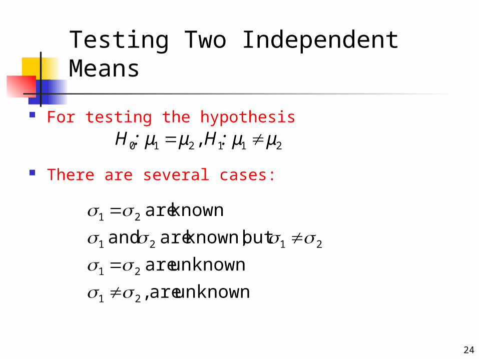
For testing the hypothesis

There are several cases:

unknown are ,

unknown are

but known, are and

known are

21

21

2121

21

211210 , μ: μHμ: μH

25


)1,0(~)()(

2

22

1

21

2121 N

n

σ

n

σ

μμXXZ

2 population from taken sample theof size

2 population of variance

2 population ofmean

2 population from taken sample theofmean


1 population of variance

1 population ofmean

1 population from taken sample theofmean where

2

22

2

2

1

21

1

1

n

σ

μ

X

n

σ

μ

X

26

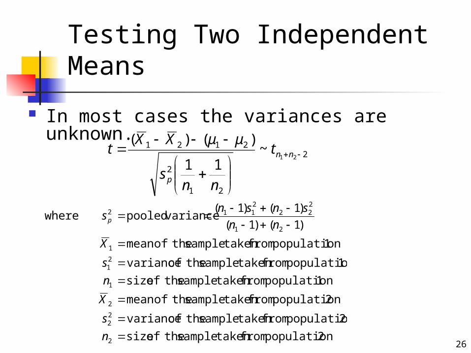
In most cases the variances are unknown.


2

21

2

212121

~11

)()(

nn

p

t

nns

μμXXt


2 population from taken sample theof variance



1 population from taken sample theof variance


)1()1(

)1()1( variancepooled where

2

22

2

1

21

1

21

222

2112

n

s

X

n

s

X

nn

snsns p

27


Output from t test for TV watching hours

Independent Samples Test

20.261.000

6.455 6.569884 870.228

.000 .000

1.092 1.092

.169 .166

.760 .7661.424 1.418

FSig.

Levene's Test forEquality of Variances

tdfSig. (2-tailed)

Mean Difference

Std. Error Difference

LowerUpper


t-test for Equalityof Means


Equal variances assumedEqual variances

not assumed

28

In the output, there are two difference versions of the t test. One makes the assumption that the variances in

the two populations are equal; the other does not.

Both tests recommend to reject the hypothesis with a significant level less than 0.0005.

The two-tailed test used in the two tests. Testing the equality of two variances will be

given next section.


29

The 95% confidence interval for the true difference is [0.77, 1.42] for equal variances not assumed, [0.76, 1.42] for the equal variances assumed.

Both the intervals do not cover the value 0, we should reject the hypothesis.


30

F test for equality of Two Variances

1,122

21

21~ nnF

s

sF

2 sample from freedom of degree1

1 sample from freedom of degree1



2 sample of variance

1 sample of variance where

2

1

2

1

22

21

n

n

n

n

s

s

31


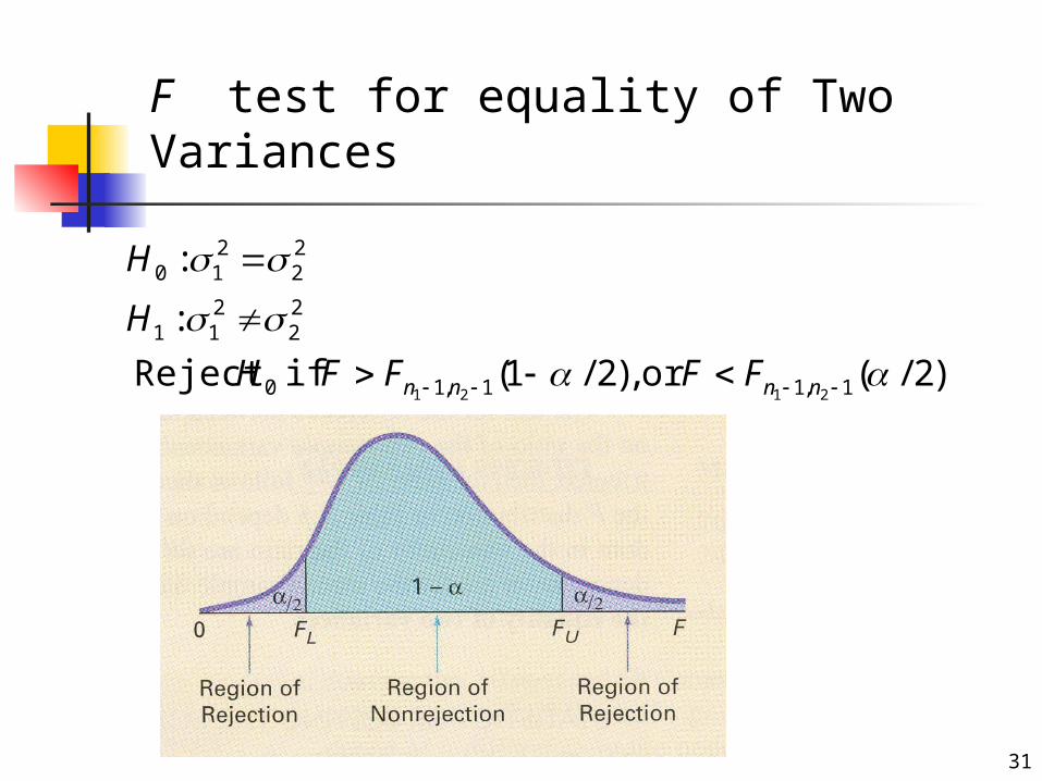
)2/(or ,)2/1( if Reject

:

:

1,11,10

22

211

22

210

2121

nnnn FFFFH

H

H

32


33


Group Statistics

469 3.40 2.491 .115411 2.35 1.866 .092

Use Internet?NoYes


N MeanStd.

DeviationStd. Error

Mean

From the results below we have

The critical value is close to 1.00 that implies to reject the hypothesis that two populations have the same variance.

782118661

4912F

2

2

..

.

34

Levene’s test for equality of variances

The SPSS report used the Levene’s test (1960) that is used to test if k samples have equal variances.

Equal variances across samples is called homogeneity of variance.

The Lenene’s test is less sensitive than some other tests.

The SPSS output recommends to reject the hypothesis.

35

Effect Outliers


25.449.000

7.013 7.145878 857.737

.000 .000

1.053 1.053

.150 .147

.758 .7631.347 1.342

FSig.


tdfSig. (2-tailed)

Mean Difference


LowerUpper





not assumed

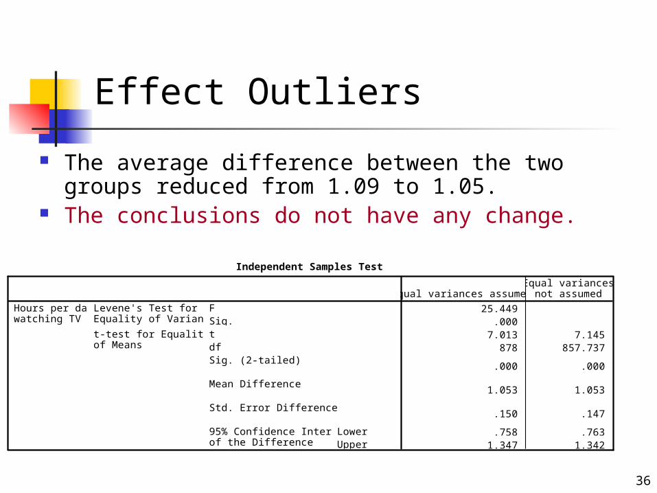
Some one reported watching TV for very long time, including 24 hours a day.

Removed observations where the person watch TV for more than 12 hours.

36

Effect Outliers


25.449.000

7.013 7.145878 857.737

.000 .000

1.053 1.053

.150 .147

.758 .7631.347 1.342

FSig.


tdfSig. (2-tailed)

Mean Difference


LowerUpper





not assumed

The average difference between the two groups reduced from 1.09 to 1.05.

The conclusions do not have any change.

37

Introducing More Variables

Group Statistics

734 51.75 18.857 .696653 40.79 13.212 .517733 12.05 2.702 .100

652 14.55 2.523 .099

356 40.80 13.960 .740532 43.74 13.481 .584171 40.98 11.990 .917238 43.38 12.498 .810

Use Internet?NoYesNoYes

NoYesNoYes

Age of respondent

Highest year of schoolcompleted

Number of hours workedlast week

Number of hours spouseworked last week

N MeanStd.

DeviationStd. Error

Mean

Let us consider more related variables to study on the TV watching time

Consider age, education, working hours.

38



131.217 .000 12.388 1385 .000 10.957 .885 9.222 12.692

12.637 1314.977 .000 10.957 .867 9.256 12.658

7.327 .007 -17.752 1383 .000 -2.503 .141 -2.779 -2.226

-17.823 1379.733 .000 -2.503 .140 -2.778 -2.227

.441 .507 -3.136 886 .002 -2.936 .936 -4.774 -1.099

-3.114 742.904 .002 -2.936 .943 -4.787 -1.085

1.050 .306 -1.948 407 .052 -2.400 1.232 -4.822 .022

-1.961 375.077 .051 -2.400 1.224 -4.806 .006

Equal variances assumedEqual variances notassumedEqual variances assumedEqual variances notassumedEqual variances assumedEqual variances notassumedEqual variances assumedEqual variances notassumed

Age of respondent

Highest year of schoolcompleted

Number of hours workedlast week

Number of hours spouseworked last week

F Sig.


t dfSig.

(2-tailed)Mean

DifferenceStd. ErrorDifference Lower Upper


Difference

t-test for Equality of Means

We reject the hypothesis that in the population the two groups have the same average age, education, and hours.

Internet users are significantly younger, better educated, and work more hours per week.

39


Date post:	13-Dec-2015
Category:	Documents
Upload:	berenice-willis
View:	215 times
Download:	2 times

1 Testing a Hypothesis about means The contents in this chapter are from Chapter 12 to Chapter 14 of...

Documents