94
1 Tests for time-to-event outcomes (survival analysis)
| Date post: | 23-Dec-2015 |
| Category: |
Documents |
| Upload: | lorraine-hoover |
| View: | 214 times |
| Download: | 0 times |

1
Tests for time-to-event outcomes (survival analysis)

2
Time-to-event outcome (survival data)
Outcome Variable
Are the observation groups independent or correlated? Modifications to Cox regression if proportional-hazards is violated:
independent correlated
Time-to-event (e.g., time to fracture)
Kaplan-Meier statistics: estimates survival functions for each group (usually displayed graphically); compares survival functions with log-rank test
Cox regression: Multivariate technique for time-to-event data; gives multivariate-adjusted hazard ratios
n/a (already over time)
Time-dependent predictors or time-dependent hazard ratios (tricky!)
3
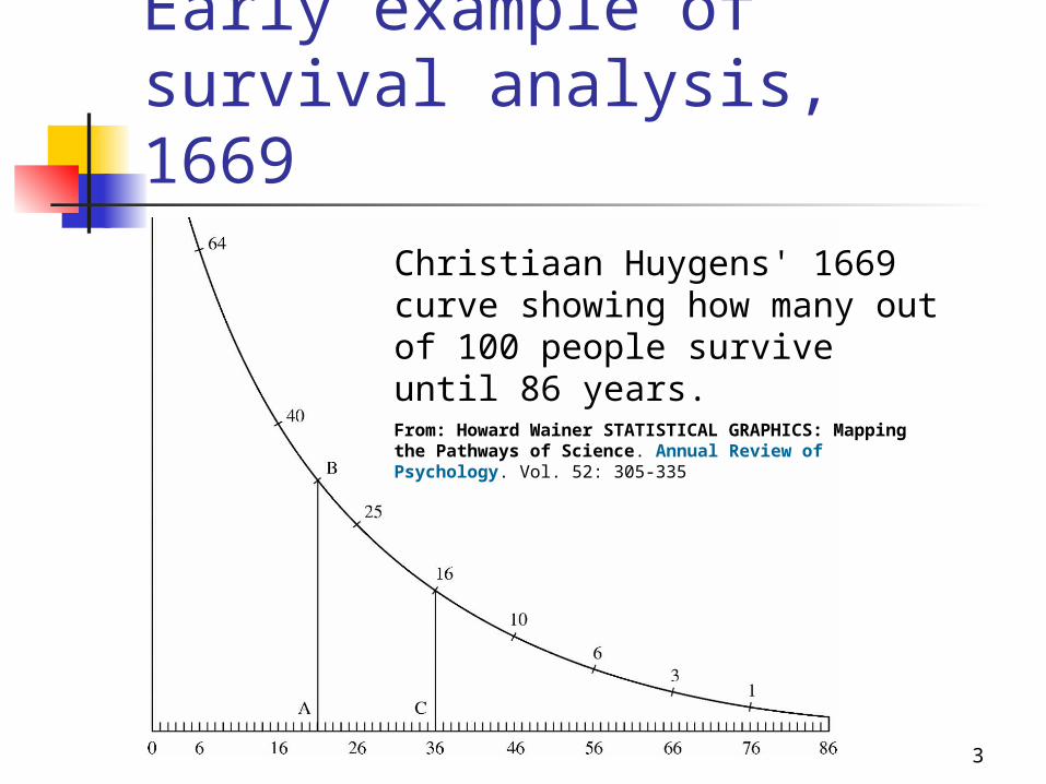
Early example of survival analysis, 1669
Christiaan Huygens' 1669 curve showing how many out of 100 people survive until 86 years.From: Howard Wainer STATISTICAL GRAPHICS: Mapping the Pathways of Science. Annual Review of Psychology. Vol. 52: 305-335
4
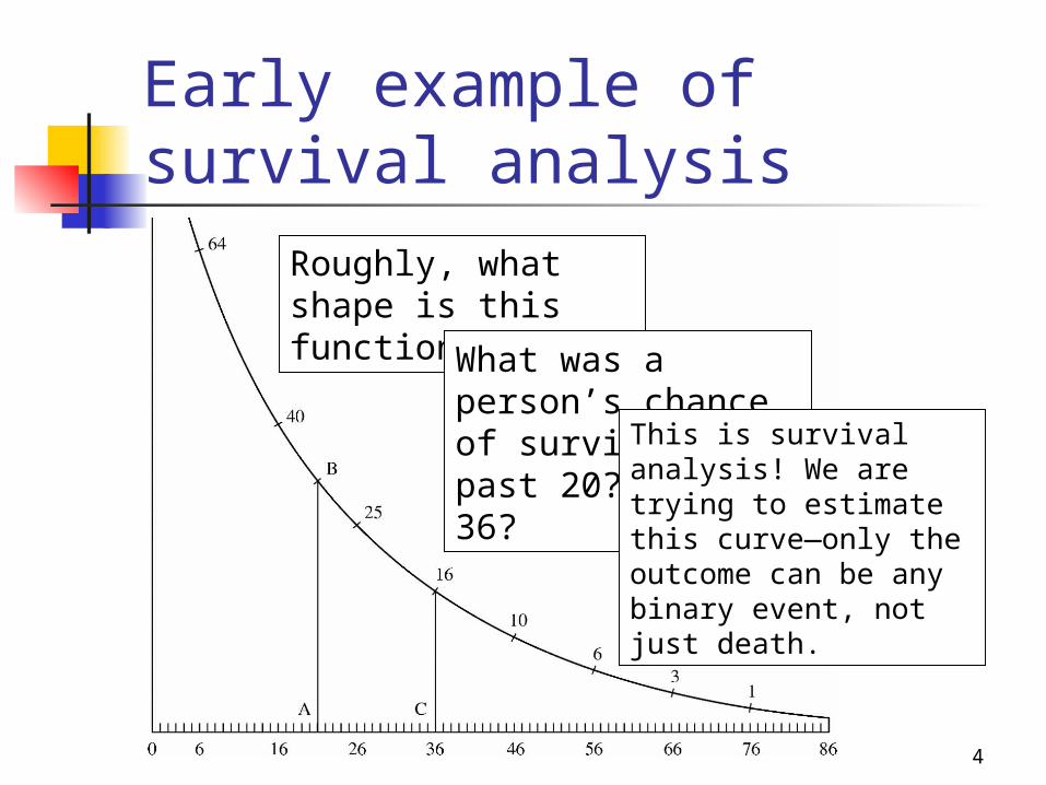
Early example of survival analysis
Roughly, what shape is this function?What was a
person’s chance of surviving past 20? Past 36?
This is survival analysis! We are trying to estimate this curve—only the outcome can be any binary event, not just death.

5
What is survival analysis? Statistical methods for analyzing
longitudinal data on the occurrence of events.
Events may include death, injury, onset of illness, recovery from illness (binary variables) or transition above or below the clinical threshold of a meaningful continuous variable (e.g. CD4 counts).
Accommodates data from randomized clinical trial or cohort study design.

Randomized Clinical Trial (RCT)
Target population
Intervention
Control
Disease
Disease-free
Disease
Disease-free
TIME
Random assignment
Disease-free, at-risk cohort
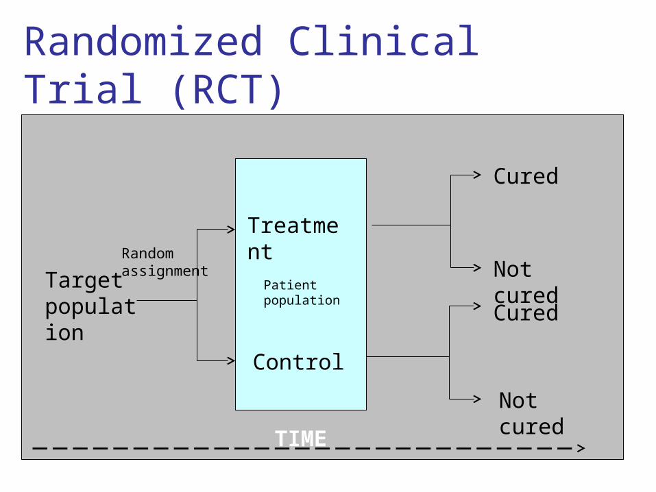
Target population
Treatment
Control
Cured
Not cured
Cured
Not cured
TIME
Random assignment
Patient population
Randomized Clinical Trial (RCT)
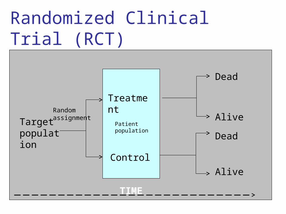
Target population
Treatment
Control
Dead
Alive
Dead
Alive
TIME
Random assignment
Patient population
Randomized Clinical Trial (RCT)

Cohort study (prospective/retrospective)
Target population
Exposed
Unexposed
Disease
Disease-free
Disease
Disease-free
TIME
Disease-free cohort

10
Examples of survival analysis in medicine
11
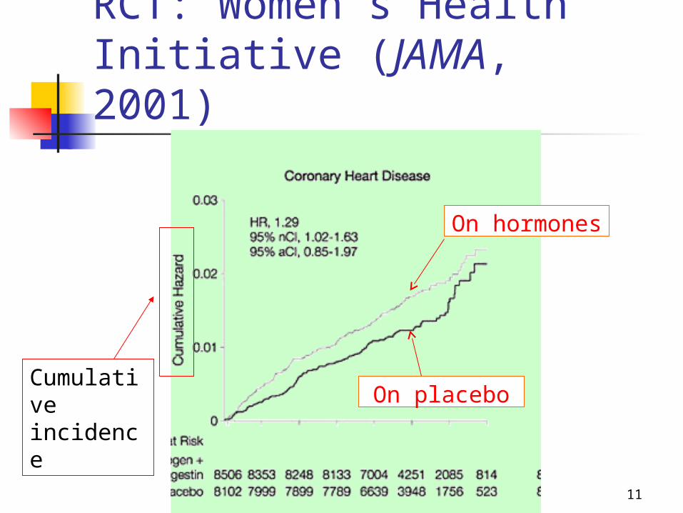
RCT: Women’s Health Initiative (JAMA, 2001)
On hormones
On placeboCumulative incidence
12
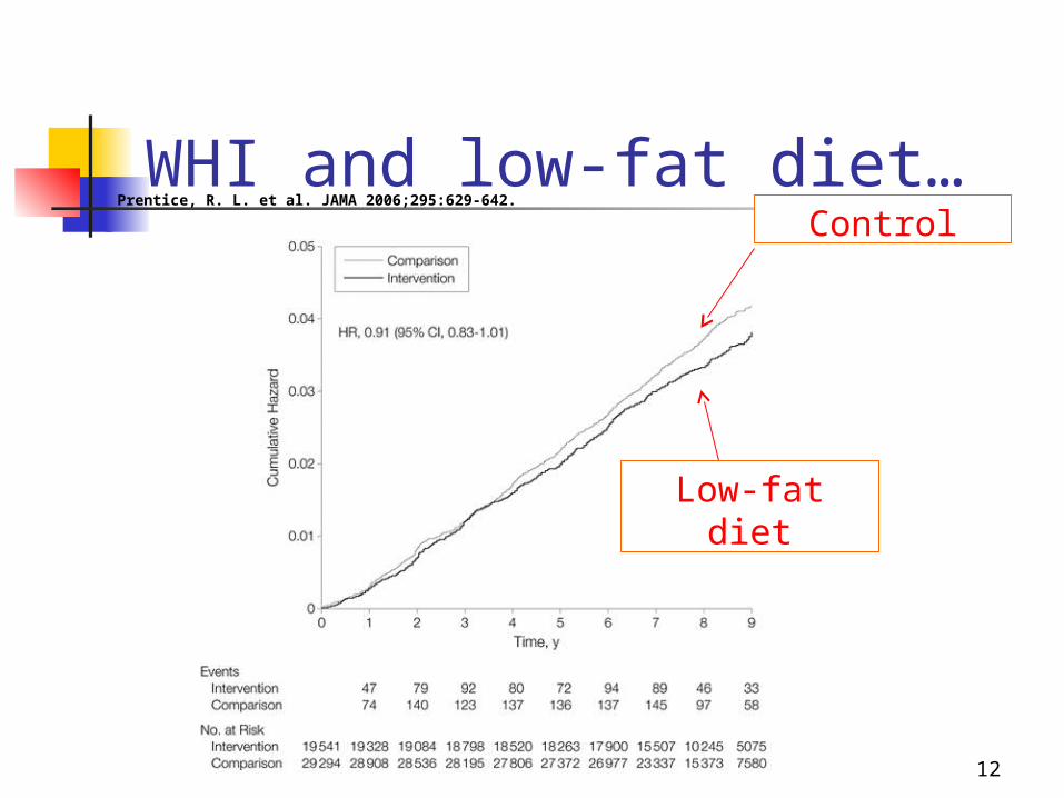
WHI and low-fat diet…Control
Low-fat diet
Prentice, R. L. et al. JAMA 2006;295:629-642.

13
Retrospective cohort study:From December 2003 BMJ: Aspirin, ibuprofen, and mortality after myocardial infarction: retrospective cohort study
14
Why use survival analysis?1. Why not compare mean time-to-
event between your groups using a t-test or linear regression?
-- ignores censoring 2. Why not compare proportion of
events in your groups using risk/odds ratios or logistic regression?
--ignores time
15
Survival Analysis: Terms Time-to-event: The time from entry into a
study until a subject has a particular outcome
Censoring: Subjects are said to be censored if they are lost to follow up or drop out of the study, or if the study ends before they die or have an outcome of interest. They are counted as alive or disease-free for the time they were enrolled in the study.
16
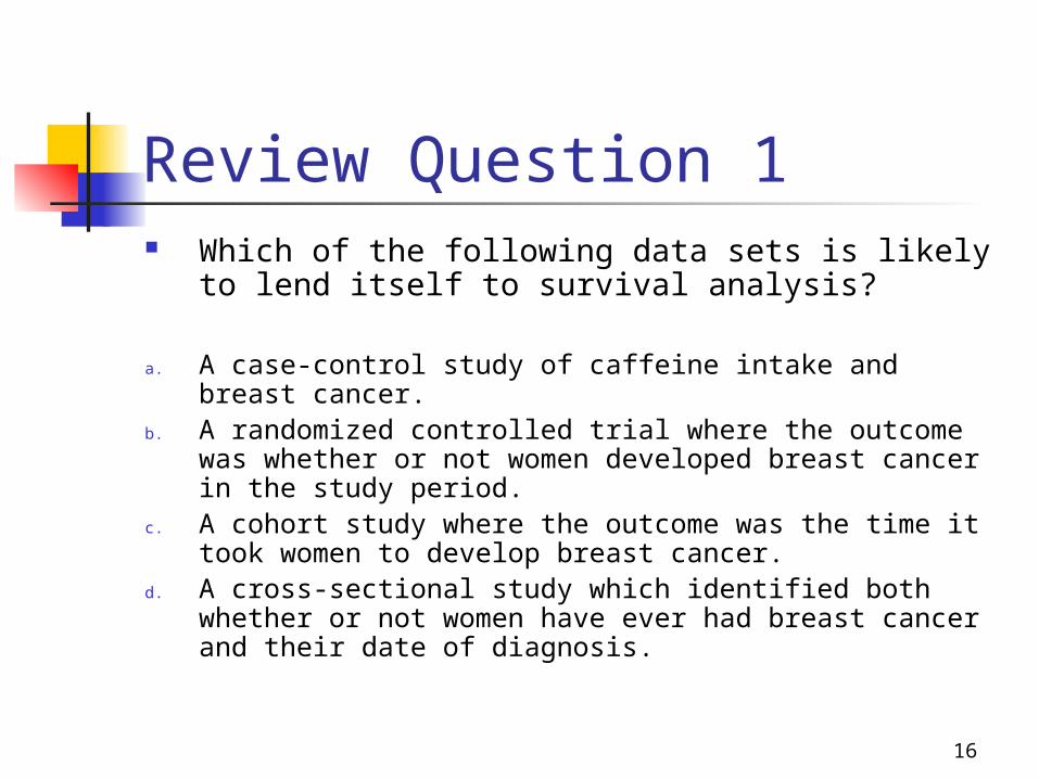
Review Question 1 Which of the following data sets is likely to
lend itself to survival analysis?
a. A case-control study of caffeine intake and breast cancer.
b. A randomized controlled trial where the outcome was whether or not women developed breast cancer in the study period.
c. A cohort study where the outcome was the time it took women to develop breast cancer.
d. A cross-sectional study which identified both whether or not women have ever had breast cancer and their date of diagnosis.

17
Introduction to Kaplan-Meier
Non-parametric estimate of the survival function:Simply, the empirical probability of surviving past certain times in the sample (taking into account censoring).
18
Introduction to Kaplan-Meier Non-parametric estimate of the
survival function. Commonly used to describe
survivorship of study population/s. Commonly used to compare two
study populations. Intuitive graphical presentation.

Beginning of study End of study Time in months
Subject B
Subject A
Subject C
Subject D
Subject E
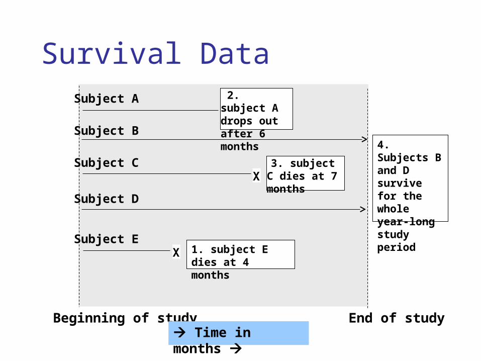
Survival Data (right-censored)
1. subject E dies at 4 months
X
100%
Time in months
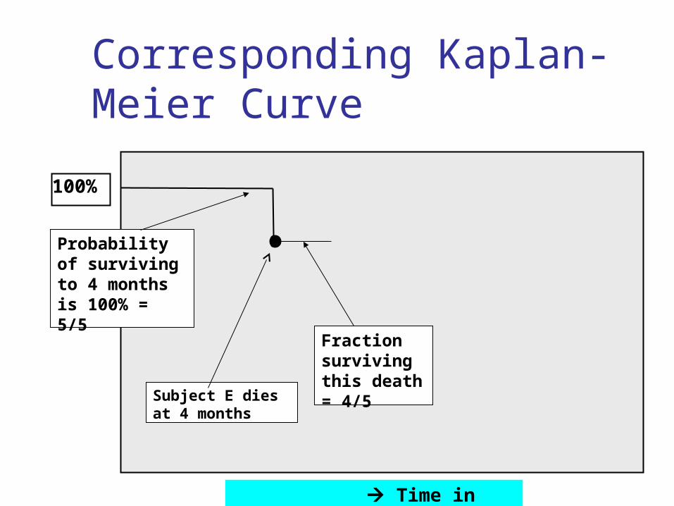
Corresponding Kaplan-Meier Curve
Probability of surviving to 4 months is 100% = 5/5
Fraction surviving this death = 4/5
Subject E dies at 4 months

Beginning of study End of study Time in months
Subject B
Subject A
Subject C
Subject D
Subject E
Survival Data 2. subject A drops out after 6 months
1. subject E dies at 4 months
X
3. subject C dies at 7 monthsX
100%
Time in months
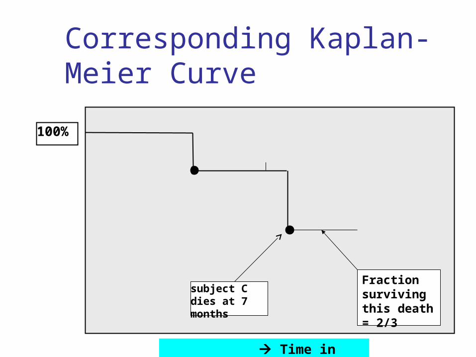
Corresponding Kaplan-Meier Curve
subject C dies at 7 months
Fraction surviving this death = 2/3
Beginning of study End of study Time in months
Subject B
Subject A
Subject C
Subject D
Subject E
Survival Data 2. subject A drops out after 6 months
4. Subjects B and D survive for the whole year-long study period
1. subject E dies at 4 months
X
3. subject C dies at 7 monthsX
24
100%
Time in months
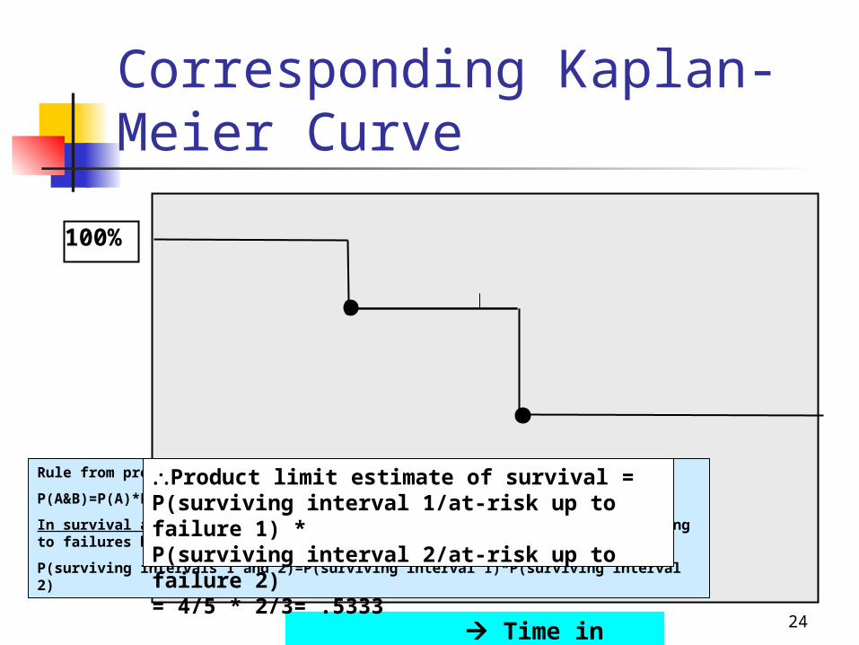
Corresponding Kaplan-Meier Curve
Rule from probability theory:
P(A&B)=P(A)*P(B) if A and B independent
In survival analysis: intervals are defined by failures (2 intervals leading to failures here).
P(surviving intervals 1 and 2)=P(surviving interval 1)*P(surviving interval 2)
Product limit estimate of survival = P(surviving interval 1/at-risk up to failure 1) * P(surviving interval 2/at-risk up to failure 2) = 4/5 * 2/3= .5333
25
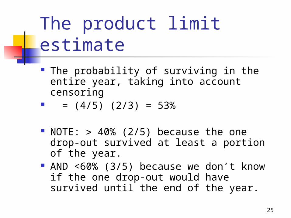
The product limit estimate The probability of surviving in the entire
year, taking into account censoring = (4/5) (2/3) = 53%
NOTE: 40% (2/5) because the one drop-out survived at least a portion of the year.
AND <60% (3/5) because we don’t know if the one drop-out would have survived until the end of the year.

26
Example 1: time-to-conception for subfertile women
“Failure” here is a good thing.
38 women (in 1982) were treated for infertility with laparoscopy and hydrotubation.
All women were followed for up to 2-years to describe time-to-conception.
The event is conception, and women "survived" until they conceived.
Example from: BMJ, Dec 1998; 317: 1572 - 1580.
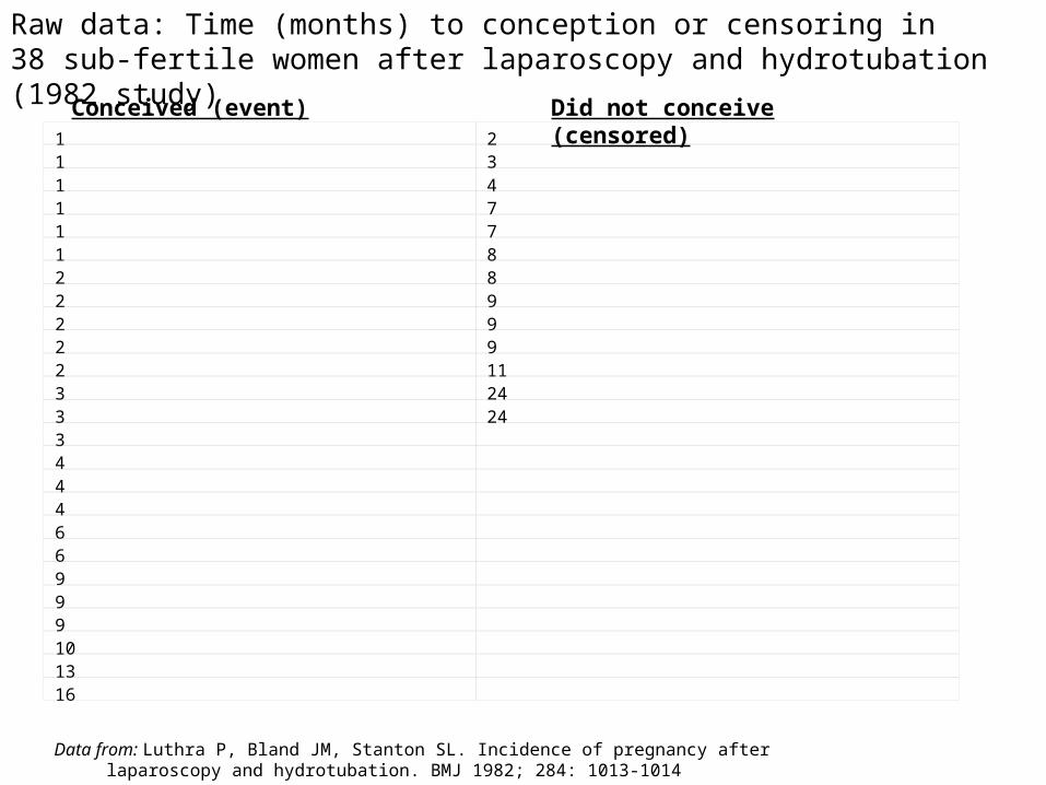
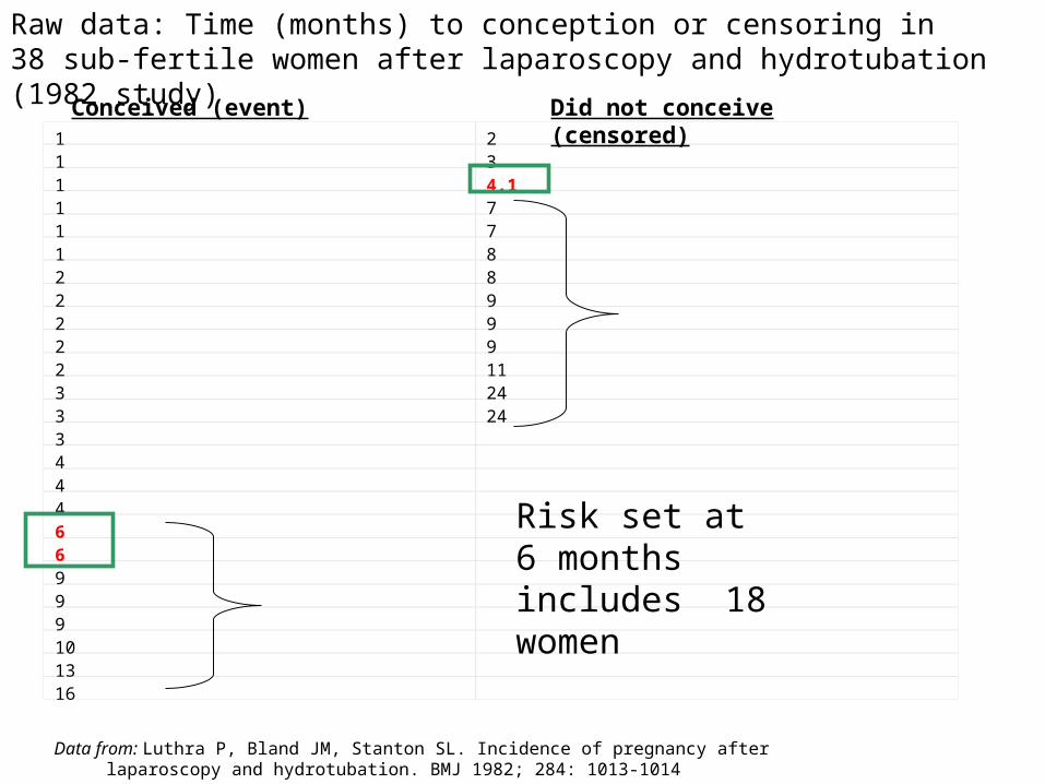
Data from: Luthra P, Bland JM, Stanton SL. Incidence of pregnancy after laparoscopy and hydrotubation. BMJ 1982; 284: 1013-1014
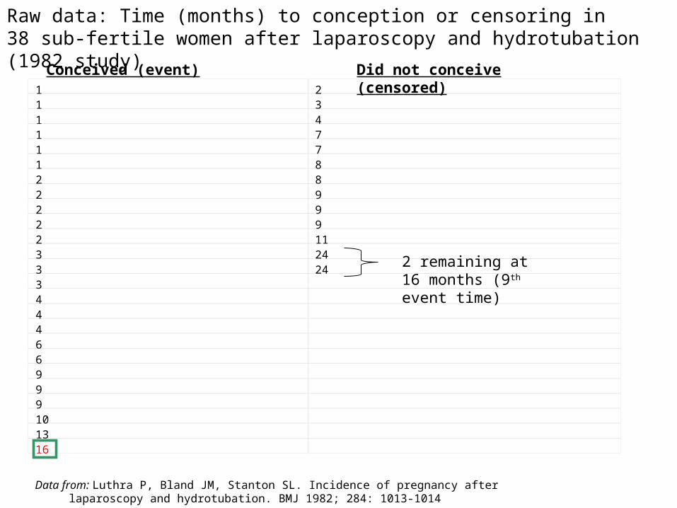
Raw data: Time (months) to conception or censoring in 38 sub-fertile women after laparoscopy and hydrotubation (1982 study)
1 21 31 41 71 71 82 82 92 92 92 113 243 243 4 4 4 6 6 9 9 9 10 13 16
Conceived (event) Did not conceive (censored)
28
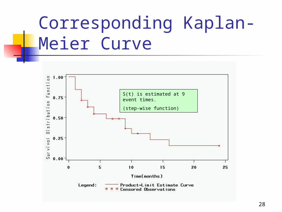
Corresponding Kaplan-Meier Curve
S(t) is estimated at 9 event times.
(step-wise function)

Data from: Luthra P, Bland JM, Stanton SL. Incidence of pregnancy after laparoscopy and hydrotubation. BMJ 1982; 284: 1013-1014
Raw data: Time (months) to conception or censoring in 38 sub-fertile women after laparoscopy and hydrotubation (1982 study)
1 21 31 41 71 71 82 82 92 92 92 113 243 243 4 4 4 6 6 9 9 9 10 13 16
Conceived (event) Did not conceive (censored)
31
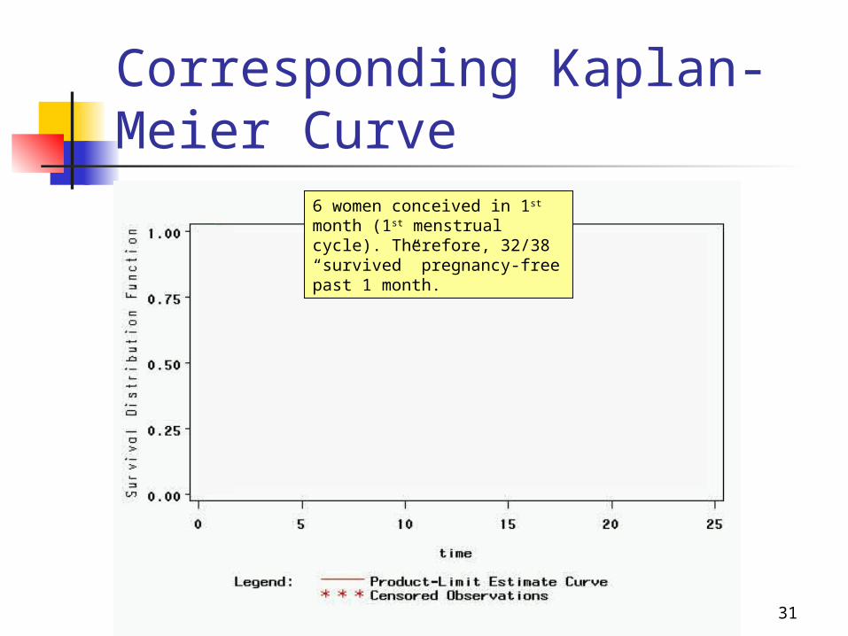
Corresponding Kaplan-Meier Curve
6 women conceived in 1st month (1st menstrual cycle). Therefore, 32/38 “survived” pregnancy-free past 1 month.
32
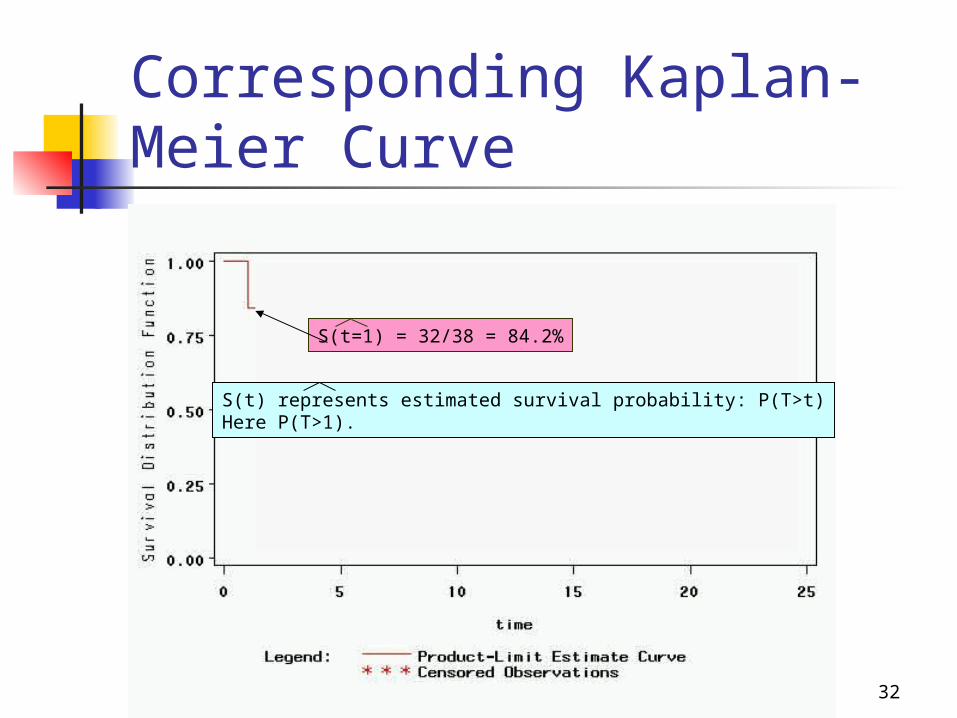
Corresponding Kaplan-Meier Curve
S(t=1) = 32/38 = 84.2%
S(t) represents estimated survival probability: P(T>t)Here P(T>1).

Data from: Luthra P, Bland JM, Stanton SL. Incidence of pregnancy after laparoscopy and hydrotubation. BMJ 1982; 284: 1013-1014
Raw data: Time (months) to conception or censoring in 38 sub-fertile women after laparoscopy and hydrotubation (1982 study)
1 2.11 31 41 71 71 82 82 92 92 92 113 243 243 4 4 4 6 6 9 9 9 10 13 16
Conceived (event) Did not conceive (censored)
Important detail of how the data were coded:Censoring at t=2 indicates survival PAST the 2nd cycle (i.e., we know the woman “survived” her 2nd cycle pregnancy-free).
Thus, for calculating KM estimator at 2 months, this person should still be included in the risk set.
Think of it as 2+ months, e.g., 2.1 months.
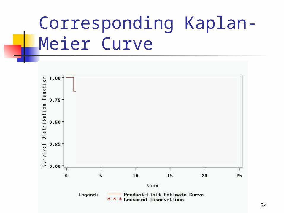
34
Corresponding Kaplan-Meier Curve

35
Corresponding Kaplan-Meier Curve
5 women conceive in 2nd month.
The risk set at event time 2 included 32 women.
Therefore, 27/32=84.4% “survived” event time 2 pregnancy-free.
S(t=2) = ( 84.2%)*(84.4%)=71.1%

Data from: Luthra P, Bland JM, Stanton SL. Incidence of pregnancy after laparoscopy and hydrotubation. BMJ 1982; 284: 1013-1014
Raw data: Time (months) to conception or censoring in 38 sub-fertile women after laparoscopy and hydrotubation (1982 study)
1 2.11 3.11 41 71 71 82 82 92 92 92 113 243 243 4 4 4 6 6 9 9 9 10 13 16
Conceived (event) Did not conceive (censored)
Risk set at 3 months includes 26 women

37
Corresponding Kaplan-Meier Curve
38
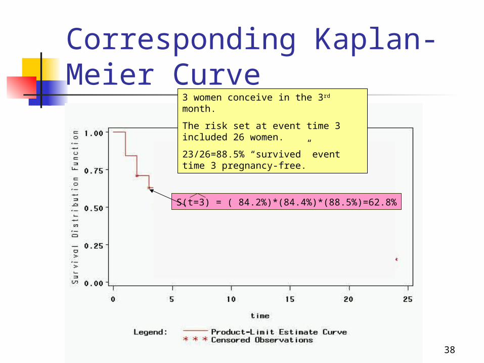
Corresponding Kaplan-Meier Curve
S(t=3) = ( 84.2%)*(84.4%)*(88.5%)=62.8%
3 women conceive in the 3rd month.
The risk set at event time 3 included 26 women.
23/26=88.5% “survived” event time 3 pregnancy-free.

Data from: Luthra P, Bland JM, Stanton SL. Incidence of pregnancy after laparoscopy and hydrotubation. BMJ 1982; 284: 1013-1014
Raw data: Time (months) to conception or censoring in 38 sub-fertile women after laparoscopy and hydrotubation (1982 study)
1 21 3.11 41 71 71 82 82 92 92 92 113 243 243 4 4 4 6 6 9 9 9 10 13 16
Conceived (event) Did not conceive (censored)
Risk set at 4 months includes 22 women
40
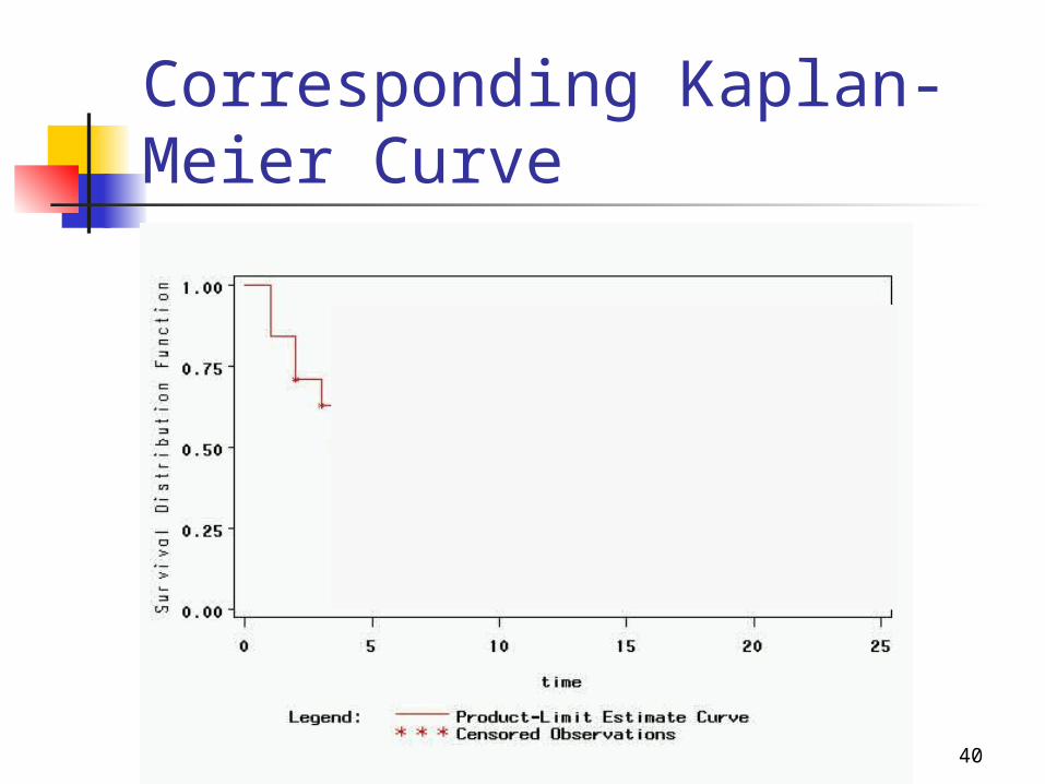
Corresponding Kaplan-Meier Curve

41
Corresponding Kaplan-Meier Curve
S(t=4) = ( 84.2%)*(84.4%)*(88.5%)*(86.4%)=54.2%
3 women conceive in the 4th month, and 1 was censored between months 3 and 4.
The risk set at event time 4 included 22 women.
19/22=86.4% “survived” event time 4 pregnancy-free.
Data from: Luthra P, Bland JM, Stanton SL. Incidence of pregnancy after laparoscopy and hydrotubation. BMJ 1982; 284: 1013-1014
Raw data: Time (months) to conception or censoring in 38 sub-fertile women after laparoscopy and hydrotubation (1982 study)
1 21 31 4.11 71 71 82 82 92 92 92 113 243 243 4 4 4 6 6 9 9 9 10 13 16
Conceived (event) Did not conceive (censored)
Risk set at 6 months includes 18 women

43
Corresponding Kaplan-Meier Curve

44
Corresponding Kaplan-Meier Curve
S(t=6) = (54.2%)*(88.8%)=42.9%
2 women conceive in the 6th month of the study, and one was censored between months 4 and 6.
The risk set at event time 5 included 18 women.
16/18=88.8% “survived” event time 5 pregnancy-free.
45
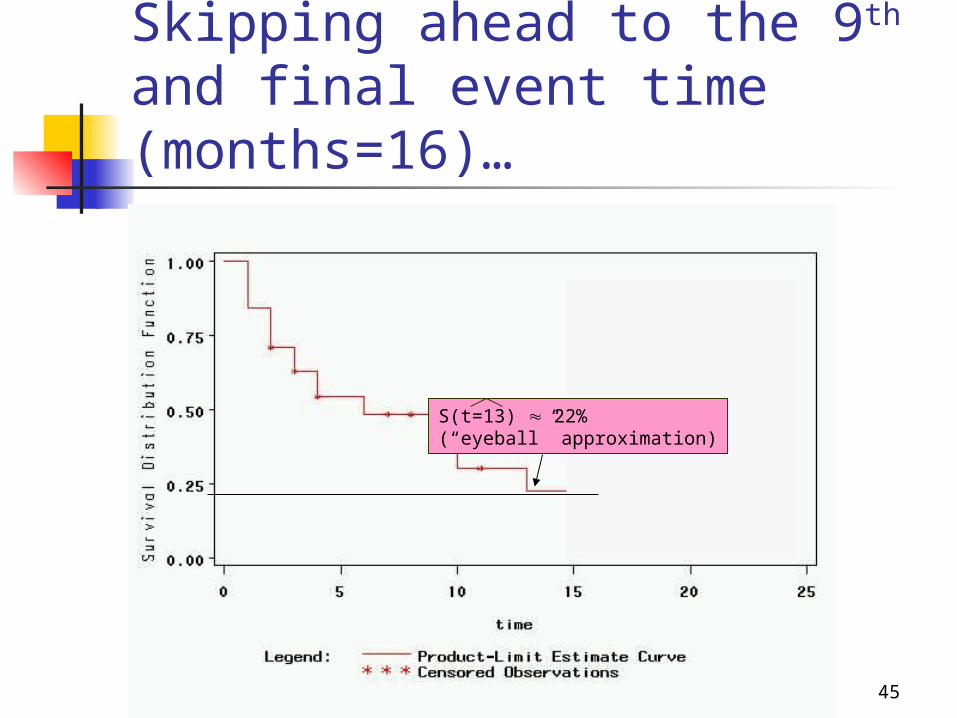
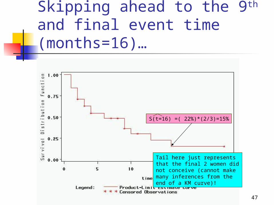
Skipping ahead to the 9th and final event time (months=16)…
S(t=13) 22%(“eyeball” approximation)
Data from: Luthra P, Bland JM, Stanton SL. Incidence of pregnancy after laparoscopy and hydrotubation. BMJ 1982; 284: 1013-1014
Raw data: Time (months) to conception or censoring in 38 sub-fertile women after laparoscopy and hydrotubation (1982 study)
1 21 31 41 71 71 82 82 92 92 92 113 243 243 4 4 4 6 6 9 9 9 10 13 16
Conceived (event) Did not conceive (censored)
2 remaining at 16 months (9th event time)
47
Skipping ahead to the 9th and final event time (months=16)…
S(t=16) =( 22%)*(2/3)=15%
Tail here just represents that the final 2 women did not conceive (cannot make many inferences from the end of a KM curve)!

Comparing 2 groups
Use log-rank test to test the null hypothesis of no difference between survival functions of the two groups

49
Kaplan-Meier: example 2
Researchers randomized 44 patients with chronic active hepatitis were to receive prednisolone or no treatment (control), then compared survival curves.
Example from: BMJ 1998;317:468-469 ( 15 August )
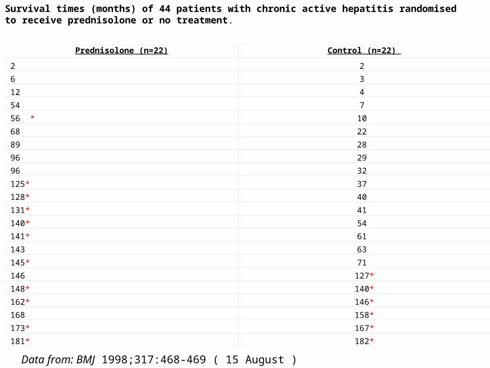
Prednisolone (n=22) Control (n=22)
2 2
6 3
12 4
54 7
56 * 10
68 22
89 28
96 29
96 32
125* 37
128* 40
131* 41
140* 54
141* 61
143 63
145* 71
146 127*
148* 140*
162* 146*
168 158*
173* 167*
181* 182*
Data from: BMJ 1998;317:468-469 ( 15 August ) *=censored
Survival times (months) of 44 patients with chronic active hepatitis randomised to receive prednisolone or no treatment.
51
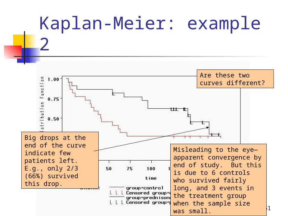
Kaplan-Meier: example 2
Are these two curves different?
Misleading to the eye—apparent convergence by end of study. But this is due to 6 controls who survived fairly long, and 3 events in the treatment group when the sample size was small.
Big drops at the end of the curve indicate few patients left. E.g., only 2/3 (66%) survived this drop.

52
Log-rank test
Test of Equality over Strata
Pr > Test Chi-Square DF Chi-Square
Log-Rank 4.6599 1 0.0309
Chi-square test (with 1 df) of the (overall) difference between the two groups.
Groups appear significantly different.

53
Caveats Survival estimates can be
unreliable toward the end of a study when there are small numbers of subjects at risk of having an event.
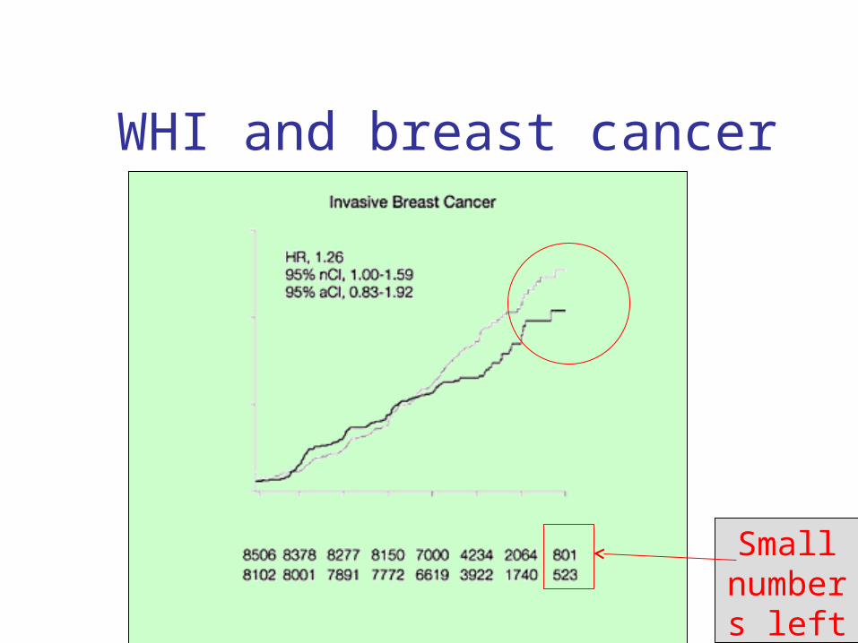
WHI and breast cancer
Small numbers
left
55
Limitations of Kaplan-Meier• Mainly descriptive• Doesn’t control for covariates• Requires categorical predictors• Can’t accommodate predictor
variables that change over time
56
Review question 2 Investigators studied a cohort of individuals who
joined a weight-loss program by tracking their weight loss over 1 year. Which of the following statistical test is likely the most appropriate test for evaluating the effectiveness of the weight loss program?
a. A two-sample t-test. b. ANOVAc. Repeated-measures ANOVAd. Chi-squaree. Kaplan-Meier methods
57
Review question 3Investigators compared mean cholesterol level between cases with heart disease and controls without heart disease. Which of the following is likely the most appropriate statistical test for this comparison?
a. A two-sample t-test. b. ANOVA.c. Repeated-measures ANOVAd. Chi-squaree. Kaplan-Meier methods
58
Review question 4What is another way to analyze the data from review question 3?
a. Logistic regressionb. Cox regressionc. Linear regressiond. Kaplan-Meier methods e. There is no other way.

59
Review question 5
Which statement about this K-M curve is correct?
a. The mortality rate was higher in
the control group than the treated group.
b. The probability of surviving past 100 days was about 50% in the treated group.
c. The probability of surviving past 100 days was about 70% in the control group.
d. Treatment should be recommended.
60
Introduction to Cox Regression
Also called proportional hazards regression
Multivariate regression technique where time-to-event (taking into account censoring) is the dependent variable.
Estimates adjusted hazard ratios. A hazard ratio is a ratio of rates
(hazard rates)

61
History “Regression Models and Life-
Tables” by D.R. Cox, published in 1972, is one of the most frequently cited journal articles in statistics and medicine
Introduced “maximum partial likelihood”
62
Distinction between hazard/rate ratio and odds ratio/risk ratio:
Hazard ratio: ratio of rates Odds/risk ratio: ratio of proportions All are measures of relative risk!
By taking into account time, you are taking into account more information than just binary yes/no.
Gain power/precision.
Logistic regression aims to estimate the odds ratio; Cox regression aims to estimate the hazard ratio
Introduction to Cox Regression
63
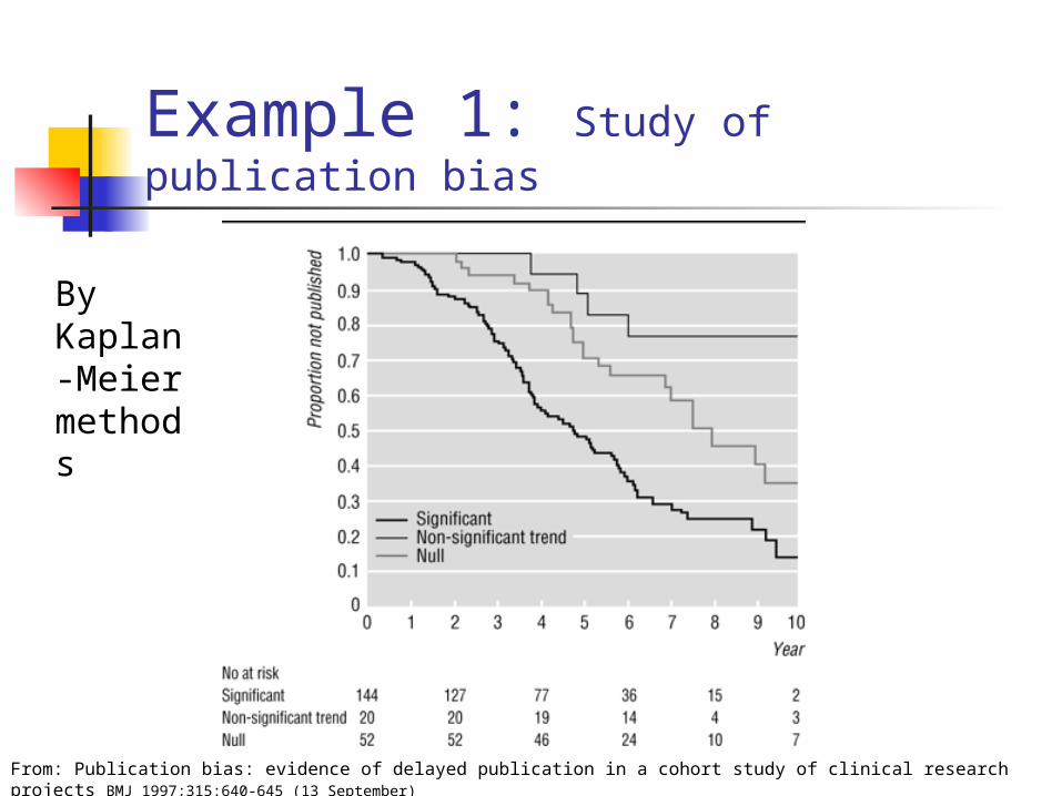
Example 1: Study of publication bias
By Kaplan-Meier methods
From: Publication bias: evidence of delayed publication in a cohort study of clinical research projects BMJ 1997;315:640-645 (13 September)

64
From: Publication bias: evidence of delayed publication in a cohort study of clinical research projects BMJ 1997;315:640-645 (13 September)
Table 4 Risk factors for time to publication using univariate Cox regression analysis
Characteristic # not published # published Hazard ratio (95% CI)
Null 29 23 1.00
Non-significant trend
16 4 0.39 (0.13 to 1.12)
Significant 47 99 2.32 (1.47 to 3.66)
Interpretation: Significant results have a 2-fold higher incidence of publication compared to null results.
Univariate Cox regression
65
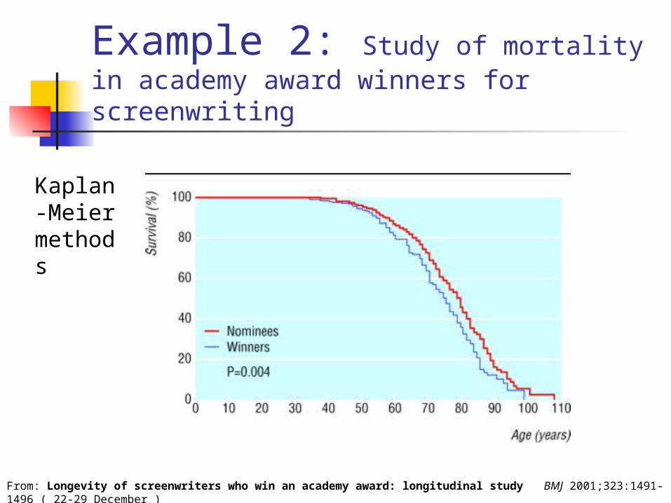
Example 2: Study of mortality in academy award winners for screenwriting
Kaplan-Meier methods
From: Longevity of screenwriters who win an academy award: longitudinal study BMJ 2001;323:1491-1496 ( 22-29 December )

Table 2. Death rates for screenwriters who have won an academy award. Values are percentages (95% confidence intervals) and are adjusted for the factor indicated Relative increase
in death rate for winners
Basic analysis 37 (10 to 70)
Adjusted analysis
Demographic:
Year of birth 32 (6 to 64)
Sex 36 (10 to 69)
Documented education 39 (12 to 73)
All three factors 33 (7 to 65)
Professional:
Film genre 37 (10 to 70)
Total films 39 (12 to 73)
Total four star films 40 (13 to 75)
Total nominations 43 (14 to 79)
Age at first film 36 (9 to 68)
Age at first nomination 32 (6 to 64)
All six factors 40 (11 to 76)
All nine factors 35 (7 to 70)
HR=1.37; interpretation: 37% higher incidence of death for winners compared with nominees
HR=1.35; interpretation: 35% higher incidence of death for winners compared with nominees even after adjusting for potential confounders
67
Characteristics of Cox Regression Can accommodate both discrete and
continuous measures of event times Easy to incorporate time-dependent
covariates—covariates that may change in value over the course of the observation period
68
Characteristics of Cox Regression, continued
Cox models the effect of covariates on the hazard rate but leaves the baseline hazard rate unspecified.
Does NOT assume knowledge of absolute risk.
Estimates relative rather than absolute risk.

69
Assumptions of Cox Regression
Proportional hazards assumption: the hazard for any individual is a fixed proportion of the hazard for any other individual
Multiplicative risk
70
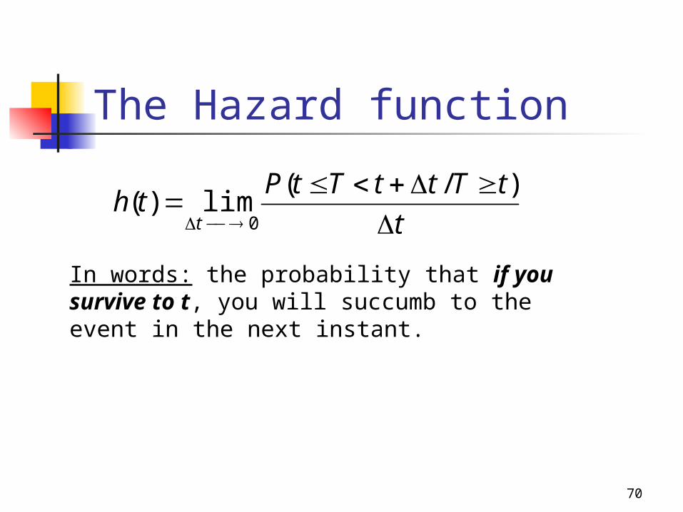
The Hazard function
t
tTttTtPth
t
)/(lim)(
0
In words: the probability that if you survive to t, you will succumb to the event in the next instant.
71
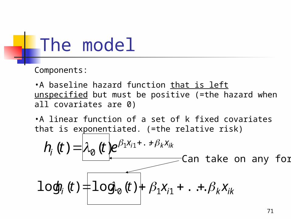
The model
ikki xxi etth ...
011)()(
Components:
•A baseline hazard function that is left unspecified but must be positive (=the hazard when all covariates are 0)
•A linear function of a set of k fixed covariates that is exponentiated. (=the relative risk)
ikkii xxtth ...)(log)(log 110
Can take on any form!

72
The model
)(...)(
...0
...0
,1111
11
11
)(
)(
)(
)( jkikji
jkkj
ikkixxxx
xx
xx
j
iji e
et
et
th
thHR
Proportional hazards:
Hazard functions should be strictly parallel!
Produces covariate-adjusted hazard ratios!
Hazard for person j (eg a non-smoker)
Hazard for person i (eg a smoker)
Hazard ratio
73
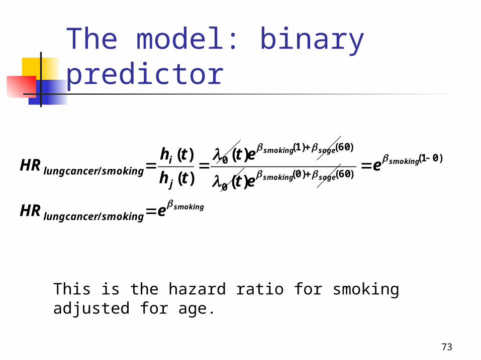
The model: binary predictor
smoking
smoking
sagesmoking
sagesmoking
eHR
eet
et
th
thHR
smokingcancerlung
j
ismokingcancerlung
/
)01(
)60()0(0
)60()1(0
/ )(
)(
)(
)(
This is the hazard ratio for smoking adjusted for age.
74
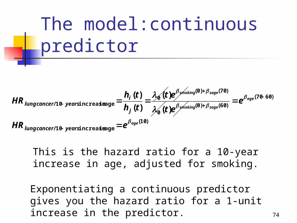
The model:continuous predictor
)10(age in increase 10/
)6070(
)60()0(0
)70()0(0
age in increase 10/ )(
)(
)(
)(
age
age
sagesmoking
sagesmoking
eHR
eet
et
th
thHR
yearscancerlung
j
iyearscancerlung
Exponentiating a continuous predictor gives you the hazard ratio for a 1-unit increase in the predictor.
This is the hazard ratio for a 10-year increase in age, adjusted for smoking.
75
Review Question 6 Exponentiating a beta-coefficient
from linear regression gives you what?
a. Odds ratiosb. Risk ratiosc. Hazard ratiosd. None of the above
76
Review Question 7 Exponentiating a beta-coefficient
from logistic regression gives you what?
a. Odds ratiosb. Risk ratiosc. Hazard ratiosd. None of the above
77
Review Question 8 Exponentiating a beta-coefficient
from Cox regression gives you what?
a. Odds ratiosb. Risk ratiosc. Hazard ratiosd. None of the above

78
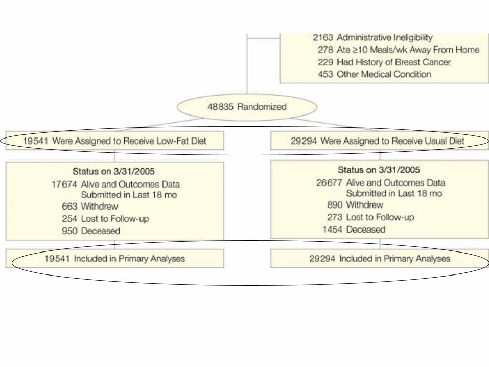
Intention-to-Treat Analysis in Randomized Trials
Intention-to-treat analysis: compare outcomes according to the groups to which subjects were initially randomized, regardless of which intervention (if any) they actually followed.

79
Intention to treat Participants will be counted in the
intervention group to which they were originally assigned, even if they: Refused the intervention after randomization Discontinued the intervention during the
study Followed the intervention incorrectly Violated study protocol Missed follow-up measurements

80
Dietary Modification Trial <20% of diet from fat >=5 servings of fruit and
vegetables >=6 servings of whole grains Primary outcomes: breast and
colorectal cancer
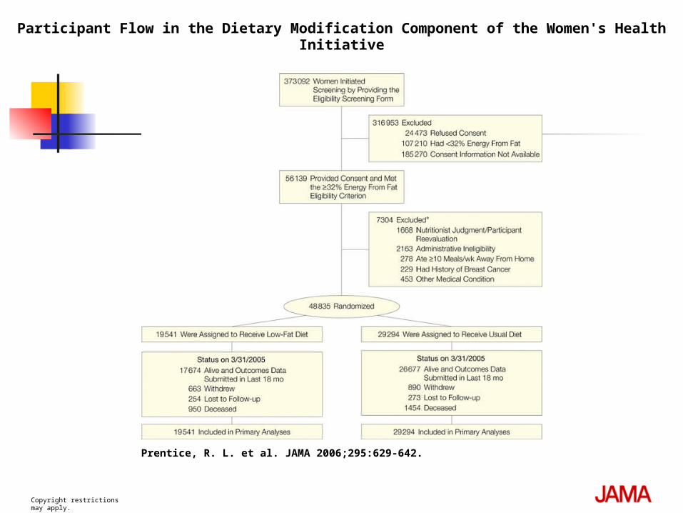
81Copyright restrictions may apply.
Prentice, R. L. et al. JAMA 2006;295:629-642.
Participant Flow in the Dietary Modification Component of the Women's Health Initiative
83
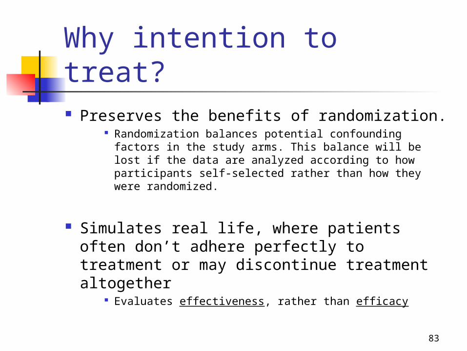
Why intention to treat? Preserves the benefits of randomization.
Randomization balances potential confounding factors in the study arms. This balance will be lost if the data are analyzed according to how participants self-selected rather than how they were randomized.
Simulates real life, where patients often don’t adhere perfectly to treatment or may discontinue treatment altogether
Evaluates effectiveness, rather than efficacy
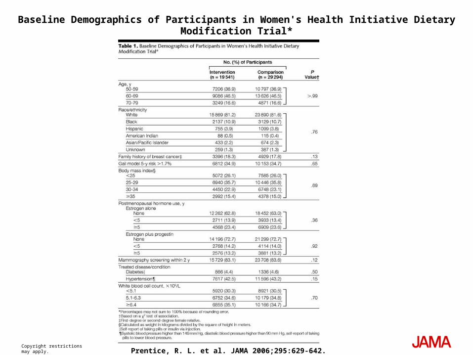
Copyright restrictions may apply.Prentice, R. L. et al. JAMA 2006;295:629-642.
Baseline Demographics of Participants in Women's Health Initiative Dietary Modification Trial*

Benefits of randomization…
86Copyright restrictions may apply.
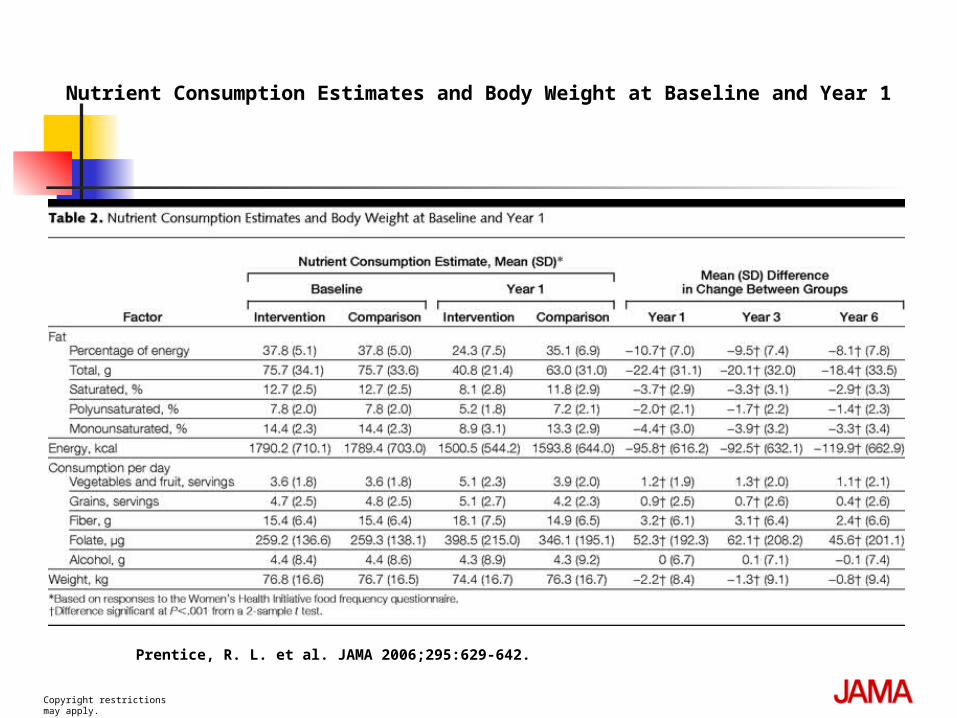
Prentice, R. L. et al. JAMA 2006;295:629-642.
Nutrient Consumption Estimates and Body Weight at Baseline and Year 1

Real-world effectiveness…
Only 31 percent of treatment participants got their dietary fat below 20% in the first year.
88
Effect of intention to treat on the statistical analysis Intention-to-treat analyses tend to
underestimate treatment effects; increased variability due to switching “waters down” results.
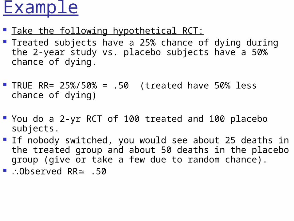
Example Take the following hypothetical RCT: Treated subjects have a 25% chance of dying during the 2-
year study vs. placebo subjects have a 50% chance of dying.
TRUE RR= 25%/50% = .50 (treated have 50% less chance of dying)
You do a 2-yr RCT of 100 treated and 100 placebo subjects. If nobody switched, you would see about 25 deaths in the
treated group and about 50 deaths in the placebo group (give or take a few due to random chance).
Observed RR .50

90
Example, continued BUT, if early in the study, 25 treated subjects
switch to placebo and 25 placebo subjects switch to control.
You would see about 25*.25 + 75*.50 = 43-44 deaths in the placebo
group And about
25*.50 + 75*.25 = 31 deaths in the treated group
Observed RR = 31/44 .70Diluted effect! (but not biased)

91
The researchers factored this into their power calculation… The study was powered to find a
14% difference in breast cancer risk between treatment and control.
They assumed a 50% reduction in risk with perfect adherence, but calculated that this would translate to only a 14% reduction in risk with imperfect adherence.

92
Alternatives to ITTPer-protocol analysis
Restricts analysis to only those who followed the assigned intervention until the end.
Treatment-received analysis Censored analysis: Subjects are dropped from the
analysis at the time of stopping the assigned treatment
Transition analysis: e.g., controls who cross over to treatment contribute to the denominator for the control group until they cross over; then they contribute to the denominator for the treatment group.
But becomes an observational study…
93
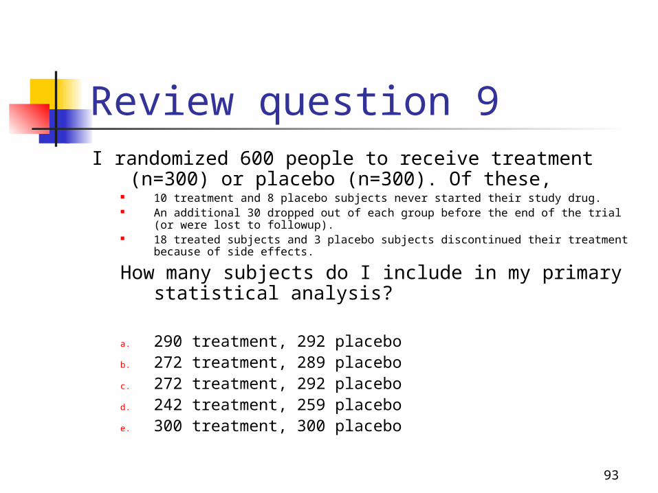
Review question 9I randomized 600 people to receive treatment
(n=300) or placebo (n=300). Of these, 10 treatment and 8 placebo subjects never started their study drug. An additional 30 dropped out of each group before the end of the trial (or were
lost to followup). 18 treated subjects and 3 placebo subjects discontinued their treatment because
of side effects.
How many subjects do I include in my primary statistical analysis?
a. 290 treatment, 292 placebob. 272 treatment, 289 placeboc. 272 treatment, 292 placebod. 242 treatment, 259 placeboe. 300 treatment, 300 placebo
94
Homework Finish reading textbook (if not
already done!) Homework 9 Read intention-to-treat article (on
Coursework) Review for the final exam


