1

1.

The aggregate approach to innovation diffusion:

the Bass Model

1.1 Introduction

Modelling and forecasting the diffusion of innovations is a broad research topic,

whose importance is confirmed by the wealth of publications regarding it. With more

than 4000 publications since the 1940, it has been said that “no other field of

behavioural science research represents more effort by more scholars in more

disciplines in more nations” (Rogers, 2003). This is a theme of both practical and

academic interest as demonstrated, for example, by the considerable share of marketing

and economic research devoted to it, which denotes not only the strategic importance of

new products and technologies in triggering the growth of an economy, but also the role

of diffusion in helping managers to plan more efficiently their strategies, by anticipating

the development of product demand (Mahajan and Muller, 1979).

Mahajan and Muller (1979) have stated that the purpose of a diffusion model is to

depict the successive increases in the number of adopters given a set of potential

adopters over time and predict the development of a diffusion process already in

progress. Shaikh, Rangaswamy and Balakrishnan (2005) have noticed that diffusion

modelling is important both for firms that introduce new products and for firms that

offer complementary or substitute products: for example, the time path of adoptions of

iPod is important not only for Apple computer but also for competitors, like Sony, and

firms that produce complementary goods, such as speakers, ear phones and carrying

cases.

2

The success of an innovation depends on various factors that may be both internal

and external. Given the great complexity of these factors, the rate of failure of new

products is quite high: for example Mahajan, Muller and Wind (2000) have reported

that this rate may vary in the range of 40 to 90 percent. Today, the shortening of product

life cycles, the increasing level of competition between firms and products, the need to

plan the likely existence of several successive generations of a new product and thus to

manage resources and commitments, require a timely investigation on the features of a

new product growth, in terms of its speed and dimension. The fundamental marketing

concept underlying the employment of new product growth models is the product life

cycle (see Wind, 1982): the product life cycle hypothesizes that sales of a new product

are characterised by stages of launch, growth, maturity and decline, miming the life

cycle of a biologic organism.

Diffusion models are typically concerned with the representation of this life cycle in

the context of sales forecasting: however, they also may be used for descriptive and

normative purposes. For example, according to the perspective presented by Muller,

Mahajan and Peres (2007) the current trend on diffusion research seems to be

increasingly focused on managerial diagnostics, able to reveal the basic structures of a

market, to allow comparisons with other contexts, and to help firms to anticipate and

prepare for possible scenarios in the future.

If the marketing and management fields played and still play a central role in

defining the boundaries and the directions of this research, it is also true that the great

interest towards innovation diffusion processes may be due to the opportunity to

connect and involve many other scientific disciplines such as economics, technological

3

forecasting, technology management, organizational behaviour, social sciences, physics,

mathematics and statistics.

Indeed, the diffusion of an innovation is primarily a social phenomenon, whose

complexity may be better understood through the contribution of various scientific

areas. Traditionally, it has been defined as the process by which an innovation is

communicated through certain channels among the members of a social system (Rogers,

2003). As such, it consists of four central elements, the innovation, the communication

channels, time and the social system.

In one of the most famous reviews of diffusion models Mahajan, Muller and Bass

(1990) argued that the main focus of diffusion theory is on communication channels,

that are the means by which information about an innovation is transmitted to or within

the social system. These means may be both formal, like mass media and advertising

and informal, like interpersonal communication.

In particular, “interpersonal communications, including nonverbal observations, are

important influences in determining the speed and shape of the diffusion process in a

social system” (Mahajan, Muller and Bass,1990).

The formal representation of these processes has historically used epidemic models

borrowed from biology, like the logistic equation, in which the social contagion

represents the driving factor of growth. The logistic equation was formulated for the

first time by Verhulst in 1838 and was originally used in natural sciences for describing

growth processes, like the spread of a disease. In 1925 the biologist Pearl called the

attention on the fundamental fact that all growth processes can be adequately described

through this equation, that gives rise to the typical s-shaped curve. Fisher and Pry

4

(1971) and Meade and Islam (1998) demonstrated the usefulness of the normalized

logistic equation in representing the diffusion of basic technologies. Marchetti (1980)

noted that innovation diffusion is basically a learning process, and learning, being a

process of growth, may be conveniently represented through the logistic curve.

Moreover, Modis (1992) demonstrated the complete equivalence between the logistic

curve and the learning curve (learning by doing). Devezas (2005) has highlighted that

the logistic equation represents one of the most powerful technological forecasting

tools, almost a “natural law” of innovation diffusion, due to its success in representing

dynamics of change within markets and industries. The s-curve is the link between a

broad literature about economic dynamics of technical change in which innovations and

the response to them are the consequences of market processes (Metcalfe, 2005).

The rationale behind the use of this equation in new product context is that an

innovation spreads in a social system through communication like an epidemic disease

through the mechanism of contagion between persons. A direct inspection of aggregate

diffusion data sets suggests that this type of models is appropriate: in fact, the

cumulative adoption of an innovation approximately follows an s-shape (or logistic)

path. Many contributions helped to clarify that diffusion processes are essentially driven

by learning through imitation. Probably one of the first to formalize this idea was the

french lawyer Tarde, whose major work is “Le lois de l’imitation” (1890). In this work

Tarde stated that the imitation process can represent a general law of social change. He

clarified that invention (in his terminology indicates the origination of novelty) is a

necessary condition of change but the actual change occurs only when a large number

of persons begins the adoption process he termed imitation. Diffusion processes as the

result of an imitative behaviour find a direct connection with a social psychological

5

theory called social learning theory. Founded by Bandura (1971), the social learning

approach looks outside of the individual and tries to explain changes of behaviour as

determined by information exchanges with others. Another noteworthy contribution in

the economic reasoning was given by Veblen in “The theory of Leisure Class” (1971),

recognising imitation as a structural element of individual economic behaviour.

The central role of imitation in explaining diffusion processes and the possibility to

represent them with the logistic curve are common elements of all the research

approaches on innovation. Rogers (2003) has stressed that this research started in a

series of independent studies during its first several decades. Despite the specificity of

these approaches to diffusion, each of these reached similar findings: in particular that

the diffusion of an innovation follows an s-shaped curve over time.

Among these streams of research, the marketing diffusion has become particularly

strong since the 1970s. Pioneering works in this area are those of Mansfield (1962),

reproducing the Verhulst structure, Fourt and Woodlock (1960), Bass (1969). During

the last 25 years, many reviews of diffusion models have been developed. Among these,

we can remember Mahajan and Muller (1979), Mahajan, Muller and Bass (1990),

Mahajan, Muller and Bass (1995), Mahajan, Muller and Wind (2000), Meade and Islam

(2001), Meade and Islam (2006), Hauser, Tellis and Griffin (2006), Chandrasekaran and

Tellis (2006), Muller, Peres, Mahajan (2007).

Interestingly, all these reviews are especially referred to the most known and

employed diffusion model, the Bass model, BM, which offered the theoretical and

empirical evidence for the existence of the s-shaped pattern to represent the first

purchase growth of a new product in marketing (Mahajan, Muller and Wind, 2000). The

purpose of this model is to depict and predict the development of this growth process

6

through time, when it is already in progress. Since its publication in Management

Science in 1969, the BM has been widely used both in academic research and practical

applications, proving its reliability in forecasting the diffusion of new products in

several industrial sectors, such as industrial technology, agriculture, pharmaceutics,

durable goods sector. As declared in the article title “A new product growth for

consumer durables”, this model was originally designed only for durable goods.

However, it has proven to be appliable to services too. The diffusion of services has

been modeled as if they were durable goods, including the case of cellular phones

(Krishnan, Bass and Kumar 2000), cable TV (Lilien, Rangaswamy and Van den Bulte

2000), online banking (Hogan, Lemon and Libai 2003), energy (Guseo, Dalla Valle and

Guidolin 2007), email services (Montgomery, 2001). Showing that the Bass model may

be applied with success also in the case of services’ diffusion has been very important,

since most innovations today in fact are services. Libai, Muller and Peres (2006) remind

that the service sector in the USA employs most of the work force, is responsible for

more than 80 % of the GDP and is growing faster than the good sector.

This chapter is dedicated to an extensive treatment of the Bass model. Section 1.2 is

dedicated to present the formal structure of the Bass model, highlighting some

theoretical assumptions and some relevant aspects for strategic evaluations and

forecasts. Section 1.3 deals with the issue of statistical implementation of the model and

proposes two examples of its concrete application to time series data. Section 1.4

presents the most famous and useful generalization of the Bass model, the Generalized

Bass model, that incorporates marketing mix variables and other exogenous factors by

the means of a general intervention function x(t) . Two applications are provided also

for this model. Section 1.5 reviews the interesting themes of spatial diffusion and

7

successive generations of product, while section 1.6 summarises some proposals of

refinement and extension of the Bass model, that according to the most recent reviews

on innovation diffusion models would deserve a deeper investigation.

1.2 The Bass Model

The Bass model, BM, describes the life cycle of an innovation, depicting its

characterising phases of launch, growth and maturity, decline. Its purpose is to forecast

the development over time of a new product growth, as result of the purchase decisions

of a given set of potential adopters (market potential).

These purchase decisions are assumed to be influenced by two sources of

information, an external one, like mass media and advertising and an internal, namely

social interactions and word-of-mouth. These are “competing” sources of information,

whose effect creates two distinct groups of adopters. One group is influenced only by

the external source and we call it innovators, the other only by the internal one and

these are the imitators.

One of the great advantages associated with the BM is the concrete possibility to

explain the initializing phase of diffusion, due to the presence of innovators. Indeed,

there exists a huge literature on the role of innovators, also called “early adopters”

(Rogers, 2003), “opinion leaders” (Katz and Lazarsfeld, 1995), but the first model

formalizing their action is the BM.

In particular, it is assumed that there exists a constant level of adopters, innovators,

buying the product at the beginning of the diffusion, even if other adopters influenced

by external information are present during the whole product life cycle.

8

In this sense the BM has recognised the role of all the communication efforts realised

by firms, whereas a pure logistic approach like that of the Mansfield model does not.

The formal representation of the BM is a first-order differential equation

!z (t) = p + qz

m

"#$

%&'m ( z( ) (1)

or

!z (t) = p m " z( ) + qz

mm " z( ) (1a)

This equation tells that the variation over time of instantaneous adoptions, !z (t) , is

proportional to the residual market, m ! z( )where m is the market potential or carrying

capacity and z(t) represents the cumulative number of adoptions at time t. Notice that

the market potential m depicts the maximum number of realizable adoptions within the

life cycle and its value is assumed constant along the whole diffusion process.

The residual market is affected by two parameters, p and q. Parameter p represents

the effect of the external influence, due to the mass media communication, while

parameter q is the so called coefficient of imitation, whose influence is modulated by

the ratio z

m, that at time t = 0 is clearly zero. Note that at time t = 0 , !z (0) = pm : this is

the constant level of adopters (innovators) acting at the beginning of diffusion. Also

notice in equation (1) that innovators are present at any stage of diffusion even if with a

time decreasing share.

In equation (1a) the co-existence of the two groups of adopters is more evident: the

first term refers to innovators, while the second one represents imitators.

9

The Bass model can also be interpreted as a hazard function, that is the probability

that an event will occur at time t given that it has not occurred. We have that

!z

m " z= p + q

z

m. (2)

Equation (2) describes the conditional probability of an adoption at time t, resulting

from the sum of the probabilities of two incompatible events, p andq zm

: thus the model

excludes adoptions due to both innovative and imitative effects, assuming that the final

purchasing decision will be determined by only one influence (external or internal).

This separation of effects generates the two classes of adopters we have defined

before. We shall observe that these are latent categories, since aggregate data on

adoptions clearly do not provide evidence on this.

1.2.1 Solution of the Bass Model

If we denote y = z

m we can equivalently rewrite the Bass model with the following

equation

!y = p + qy( ) 1" y( ) (3)

or

!y + qy2+ p " q( )y " p = 0 (3a)

Notice that equation (3a) represents a particular case of a more general Riccati

equation, as analysed in Guseo (2004).

10

The real roots of the characteristic equation ax2+ bx + c = 0 defined as

ri=

!b ± b2! 4ac( )

2a are r

1= !

p

q and r

2= 1 in the BM case. In general, the terms !y

and 1! y are positive, p and q are positive too, so that r1< 0 < r

2. Therefore, the

solution’s asymptotes are !p

q and 1 under initial condition y(0) = 0 .

The proposed closed-form solution of the Bass model is a special cumulative

distribution (see in particular Figure 1)

y(t) =1! e

! p+q( )t

1+q

pe! p+q( )t

. (4)

The proportion of adoptions y(t) provided by equation (4), describes the dynamics of

the diffusion process, in terms of adoption parameters, p and q. We also can refer to the

absolute scale representation, that is to the number of adoptions, z(t) , just multiplying

equation (4) by the market potential m, acting as a scale parameter

z(t) = m1! e

! p+q( )t

1+q

pe! p+q( )t

. (4a)

Notice that limt!+"

y t( ) = r2 and therefore lim

t!+"z t( ) = mr

2, so that the asymptotic

behaviour of diffusion in absolute terms, z(t) , is controlled by the size of the market

potential m, since r2= 1 .

11

Figure 1. The Bass model, cumulative adoptions y(t). The model describes a saturation.

Previous equations indicate cumulative adoptions at time t, but if we are more

interested on period-by-period or instantaneous adoptions we will use the correspondent

first order derivative, that is the density function (see Figure 2)

!y (t) =p p + q( )

2e" p+q( )t

p + qe" p+q( )t( )

2 (5)

or the corresponding absolute version

!z (t) = mp p + q( )

2e" p+q( )t

p + qe" p+q( )t( )

2. (5a)

12

Figure 2. The Bass model: instantaneous adoptions highlight the existence of a peak, point of maximum growth of diffusion.

Instantaneous adoptions highlight the presence of a peak, that is the point of

maximum growth of the diffusion, after which the process begins to decrease. It is easy

to understand that from a strategic point of view the peak represents a very crucial stage

of a diffusion process, indicating that maturity phase of the product life cycle, after

which the decline begins. The time at which the peak occurs is given by

t* =ln q / p( )

p + q( ) (6)

where the cumulative function takes the value

z(t*) = m 1 / 2 ! p / 2q( ) . (7)

Interestingly, we may observe in equation (7) that when the peak occurs, cumulative

sales z(t) are approximately equal to m2

, because p is usually very small if compared

with q. Equation (4a) depends on initial condition z(t = 0) = 0 . However, if information

and data about the very first stages of a diffusion process are not available, the model

may be modified for overcoming this shortage

13

z(t) = m1! e

! p+q( ) t!c( )

1+q

pe! p+q( ) t!c( )

, t ! c; p,q > 0 (8)

where c is an unknown translation parameter to be estimated such that z(c) = 0 .

1.3 Implementation of the Bass model

The use of the Bass model for forecasting the diffusion of an innovation requires the

estimation of three parameters: external influence, p, internal influence, q, market

potential, m (and possibly, c). These three parameters can be estimated using

cumulative sales data: as reported by Sultan, Farley and Lehmann (1990) average

values for p and q are respectively 0.03 and 0.38. The size of the market potential m is

probably the most critical element in forecasting matters and a reliable estimation of it

should be established as soon as possible. However, several empirical studies have

demonstrated that parameter estimates, thus forecasts, are quite sensitive to the number

of data available: in other words estimates suffer the fact that data are sequentially

concentrated in the first part of the innovation life cycle. In particular, Srinivasan and

Mason (1986) have maintained that reliable estimates may be obtained if non

cumulative data include the peak, which would imply, on the contrary, a considerable

reduction of the model forecasting ability. Mahajan, Muller and Bass (1990) effectively

synthesize the problem: “parameter estimation for diffusion models is primarily of

historical interest; by the time sufficient observations have been developed for reliable

estimation, it is too late to use the estimates for forecasting purposes”.

Van den Bulte and Lilien (1997) have considered some bias in parameter estimation,

including the tendency to underestimate the market potential, whose value is generally

close to the latest observed data. Given these estimation difficulties on the one hand and

14

the need of early forecasts on diffusion on the other, Meade and Islam (2006) suggest

that the identification of factors determining the market potential would be a fruitful

area of research. Estimation aspects are also discussed in Venkatesan and Kumar

(2002), Venkatesan, Krishan and Kumar (2004) and Jiang, Bass and Bass (2006).

Empirical experience has shown that ordinary least squares technique (OLS) is non-

optimal for estimating the Bass model, because of some shortcomings including the

tendency to yield negative sign parameters (that is, negative probabilities).

Mahajan, Mason and Srinivasan and Srinivasan and Mason (1986) have proposed a

non-linear least square approach (NLS), which is generally accepted as the more

reliable non-parametric method of estimation of the Bass model (see Putsis and

Srinivasan, 2000 and Muller, Peres and Mahajan, 2007). More recently, Venkatesan and

Kumar (2002) have suggested the use of Genetic Algorithms (GAs) as an alternative to

NLS approach: the claimed superiority of GAs with respect to NLS is questioned in

Guseo and Guidolin (2007a).

Consistently with most of the literature on this issue, in this work it will be used a

NLS approach (e.g. Levenberg-Marquardt, see Seber and Wild, 1989) to estimate the

Bass model parameter: in doing so we may consider the structure of a non linear

regression model, resulting from the sum of two components

z t( ) = f !,t( ) + " t( ) (9)

where z(t) is the observed response, f (!,t) is the deterministic component,

depending on parameter

�

! " Rk and time t. The second component, !(t) , is defined as

a stochastic process representing the residual term.

The BM regressive model is therefore

15

z t( ) = m1! e

! p+q( )t

1+q

pe! p+q( )t

+ " t( ) . (10)

where z(t) is the observed data, namely cumulative number of adoptions or sales at

time t. The unknown constants m, p, q are the parameters to be estimated. In general

!(t) is a white noise process, so that residual mean is zero, M ! t( )( ) = 0 , the variance

is constant, Var ! t( )( ) = "2 and different error terms are incorrelated, !

" t( )," #t( ) = 0 ,

t ! "t . Nevertheless, the concrete application of the NLS procedure to several cases has

shown that residuals cannot be always considered incorrelated and a better

representation of !(t) would be therefore required. A possible answer to this aspect

may be given by ARMAX frameworks. See for instance Box and Jenkins (1976) and,

among others, Guseo and Dalla Valle (2005).

In the following sub-sections two examples on the statistical implementation of the

standard Bass model to new product diffusion are presented, in order to clarify some

basic aspects of the concrete application of this model to time series. The first one

concerns the diffusion of a new pharmaceutical drug in Italy, for which weekly

cumulative sales data are available, while the second one considers the adoption path of

photovoltaic solar cells in Japan. While the purpose of these two examples is purely an

illustrative one, it is interesting to notice that two very different contexts like medical

innovation and energy technologies have been chosen, to show the versatility of the

Bass model, whose application ranges over a broad set of industrial sectors, like durable

goods, services, entertainment products, medical and agricultural innovations,

technologies.

16

1.3.1 A standard Bass model for the diffusion of a new

pharmaceutical drug in Italy

This sub-section provides a simple example to describe the application of a standard

Bass model to the diffusion of a new pharmaceutical drug in Italy. Several works have

demonstrated the suitability of this model to new pharmaceuticals’ diffusion (see

Mahajan, Muller and Bass, 1990). The markets for drugs are particularly attractive for

diffusion research given the considerable level of competition between firms, the

shortened life cycles of products and the consequent search for product innovations. In a

recent review on new products’ diffusion Chandrasekaran and Tellis (2006) have

stressed that medical innovations should constitute a typical field of investigation for

diffusion research. Moreover, the acceptation of new drugs or new medical technologies

by physicians represent a classical topic of research (see for instance Coleman, Katz and

Menzel, 1966; Van den Bulte and Lilien, 2001), since it is still in doubt if the

prescriptive behaviour of physicians is mainly influenced by advertising and marketing

efforts or by contagion and network effects with other physicians.

The data analysed in this example are provided by IMS Health-Italia, cover the

period between 2005 and 2007 and refer to the weekly cumulative number of sold

packages of this drug in Italy. The product, introduced in August 2005, is normally

prescribed by physicians to prevent fetus malformations and its assumption by

expectant mothers has been also recommended by the Italian Department of Health with

the sponsorizations of informative campaigns and advertisements. The Bass model

combines the perspectives expressed in the literature on medical innovation, assuming

that adoption of a new drug can occur either because of effective marketing activity or

17

for social contagion. The application of the Bass model to our time series yields the

results summarised in Table 1.

A new pharamceutical drug in Italy (data source: IMS health)

m p q R^2 D -W

1,69092E6 0,00260509 0,0320454 99,8906 percent 0, 022114

(1,60614E6) (0,00252992) (0,0302139)

(1,7757E6) (0,00268027) (0,0338778)

Table 1: Standard Bass model estimation results. Asymptotic 95% confidence intervals into parentheses

A new drug's diffusion

t

VariablesObservedPredicted

0 30 60 90 120 1500

4

8

12

16(X 100000)

Figure 3. Cumulative observed vs. predicted values with a standard Bass model: good level of fitting.

18

A new drug's diffusion

t

VariablesObservedPredicted

0 30 60 90 120 1500

3

6

9

12

15

18(X 1000)

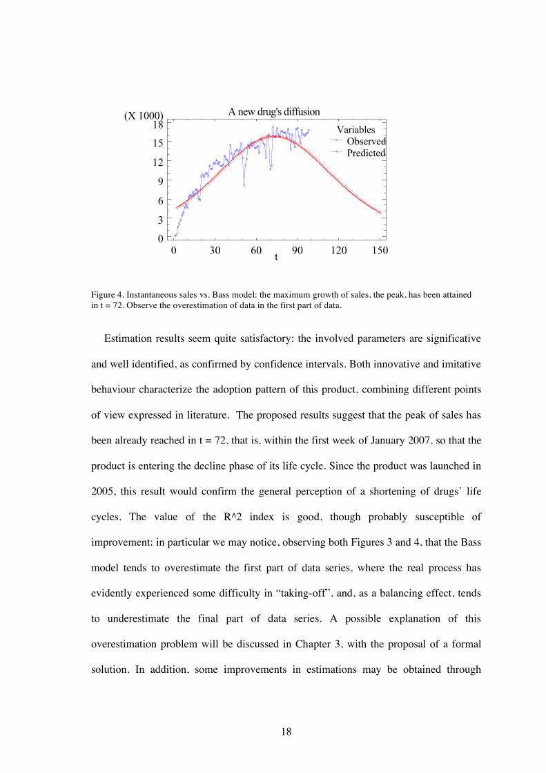
Figure 4. Instantaneous sales vs. Bass model: the maximum growth of sales, the peak, has been attained in t = 72. Observe the overestimation of data in the first part of data.

Estimation results seem quite satisfactory: the involved parameters are significative

and well identified, as confirmed by confidence intervals. Both innovative and imitative

behaviour characterize the adoption pattern of this product, combining different points

of view expressed in literature. The proposed results suggest that the peak of sales has

been already reached in t = 72, that is, within the first week of January 2007, so that the

product is entering the decline phase of its life cycle. Since the product was launched in

2005, this result would confirm the general perception of a shortening of drugs’ life

cycles. The value of the R^2 index is good, though probably susceptible of

improvement: in particular we may notice, observing both Figures 3 and 4, that the Bass

model tends to overestimate the first part of data series, where the real process has

evidently experienced some difficulty in “taking-off”, and, as a balancing effect, tends

to underestimate the final part of data series. A possible explanation of this

overestimation problem will be discussed in Chapter 3, with the proposal of a formal

solution. In addition, some improvements in estimations may be obtained through

19

further assumptions on residuals, as suggested by the value of the Durbin-Watson

statistic, whose value indicates the presence of residuals’ autocorrelation.

1.3.2 Modelling the diffusion of photovoltaic energy in Japan with a

BM

Guidolin and Mortarino (2007) have studied the diffusion of photovoltaic systems

across various world countries applying the Bass model or its extensions (here

presented in section 1.4) to the annual data of cumulative installed power, provided by

the International Energy Agency (IEA) for the period 1992-2006.

Studies and forecasts on impending oil and natural gas depletion, worsening climate

change, increasing needs of security in energy provision are inducing many countries to

put energy issues on top of their agendas and look for alternatives to fossil fuels with

increasing pressure. Among all the viable solutions, photovoltaic solar energy (PV) is

considered one of the most attractive for various reasons. The success of this energy

source, that directly converts sunlight into elecricity, is obviously driven by a

widespread adoption of photovoltaic solar cells. However, the purchase of a PV system

typically yields negative outcomes at the time of purchase, while positive outcomes are

delayed, so that the final purchase decision appears particularly complex and risky to

consumers. To overcome this problem in many countries incentive measures have been

adopted.

In recent years, industry and markets for photovoltaic cells have experienced an

unprecedented growth, so that evaluations and technological forecasts on the future

development of this sector appear crucial. In fact, current technology for solar cells

relies on silicon, whose limited availabilty is considered the major constraint for PV

20

growth. The innovation diffusion approach and specifically the Bass model have

appeared an appropriate choice for analysing this technolgical context.

The most succesful country in stimulating an adoption path is Japan, that, from being

a PV producer just for small devices like calculators and watches, became the sector

leader in less than ten years. Governmental and public institutions were required to

install PV systems at facades and on roofs. The most important program for residential

PV dissemination was the “70.000 Roofs” program, ending in 2002 after exceeding all

objectives. Today the market for PV systems in Japan is largely self-supported and

driven by market mechanisms. The most recent data on cumulative PV installations,

provided by IEA, document an installed base of about 1700 MW (USA:624, Spain:118,

Italy:50, for a direct comparison). Guidolin and Mortarino have applied a standard Bass

model with parametric origin, because data are not available for the initializing phases

of diffusion. The results of this application are summarised in Table 2.

PV diffusion in Japan (data source: IEA 1992-2006)

m p q c R^2

2778 0,0001 0,420592 5,76226 99,9865

(2535) (-0,00074) (0,404772) -12,9056

(3020) (0,00096) (0,436412) 24,4301

Table 2. Parameter estimates. Asymptotic 95% confidence intervals into parentheses.

Estimation results are quite good, in spite of some uncertainty in confidence intervals

for parameters p and c. However, the estimate of the market potential m seems rather

stable, suggesting that Japan is probably going to saturate its domestic market in less

21

than ten years, as one may observe in Figure 6. Interestingly, we may see that parameter

q presents a quite high value, pointing out the importance of the imitative component in

PV adoptions in Japan. Among the cases analysed in Guidolin and Mortarino (2007),

that of Japan is one for which the standard Bass model fits well data, avoiding the use of

more complex models. In other cases, the application of a Generalised Bass model,

presented in section 1.4, is essential for recovering the impact on diffusion of external

interventions, such as incentive measures and other forms of market stimulation. This

does not indicate that the adoption process in Japan was not characterized by external

interventions and incentive maeasures: on the contrary, it suggests that these actions

represent a structural element of the whole diffusion from its origins, so that observed

data, that is adopting behaviour, incorporate these as normal rules of the process.

Plot of Fitted Model

t

JapC

um

0 5 10 15 20 25 300

300

600

900

1200

1500

1800

Figure 5. Plot of fitted model: a standard Bass model yields satisfactory estimates, R^2= 99,98 percent.

22

PV diffusion in Japan

t

VariablesJapObsJapPred

0 5 10 15 20 25 300

0,5

1

1,5

2

2,5

3(X 1000)

Figure 6. Predicted vs. observed cumulative data: Japan is going to saturate its domestic market in

about ten years.

1.4 The introduction of marketing mix variables: the Generalized

Bass Model

Reviews on diffusion models (Mahajan and Muller, 1979; Mahajan and Wind, 1986;

Mahajan, Muller and Bass, 1990) had pointed out that a great limitation of the Bass

model was not incorporating into the model marketing mix variables under managerial

control, like price strategies and advertising. As clarified by Muller, Peres and Mahajan

(2007) this omission raised a conceptual conflict since the model provides high level of

fit and reliable forecasts just making some hypotheses on consumers’ behaviour and

without marketing mix variables, but on the other side it is clear that marketing mix

decisions exert a notable impact on new product growth. Besides, the shortening of life

cycles due to the growth of successive generations (see Norton and Bass, 1987),

especially for high technology products, increased the need of a model with control

variables incorporated.

23

Bass, Jain and Krishnan (2000) provided a notable review on several attempts trying

to incorporate control variables into diffusion models. Among these, we recall models

including price effects alone, namely Robinson and Lakhani (1975), Bass (1980),

Kalish (1985), Kamakura and Balasubramanian (1988), Jain and Rao (1990), Horsky

(1990), and advertising alone, namely Horsky and Simon (1983) and Simon and

Sebastian (1987). In particular Bass, Jain and Krishnan (2000) list some desirable

properties of a diffusion model with decision variables: it should have empirical support

and should be managerially useful, allowing a direct interpretation of parameters and

comparisons with other situations, should have a closed-form solution and be easy to

implement.

The model presenting all these properties, formalized by Bass, Krishnan and Jain

(1994), is the Generalized Bass Model, GBM. Conceived for taking into account both

price and advertsing strategies, the Generalized Bass Model enlarges the basic structure

of the Bass model by multiplying its basic structure by a very general intervention

function x t( ) = x t,!( ),! "Rk , assumed to be essentially nonnegative and integrable.

The GBM presents a surprisingly simplified structure

!z t( ) = p + qz

m

"#$

%&'m ( z( )x t( ) (11)

and its closed-form solution is, under initial condition z(t = 0) = 0

z t( ) = m1! e

! p+q( ) x "( )d"0

t

#

1+q

pe! p+q( ) x "( )d"

0

t

# (12)

24

The original form of function x(t) as designed by Bass, Krishan and Jain (1994)

jointly considers the percentage variation of prices and advertising efforts taking the

form x(t) = 1+ !1P "r (t)

Pr(t)+ !2

"A (t)

A(t), where Pr(t) and A(t) are price and advertising at

time t. One interesting feature of the GBM is that it reduces to the Bass model, when

x t( ) = 1, i.e. when there are no changes in price and advertising. Besides, if the

percentage changes in price and advertising remain the same from one period to the

next, then function x(t) reduces to a constant, yielding again the Bass model. This

would explain why the Bass model provides good parameter estimates, even without

marketing mix variables. The GBM can be estimated by a NLS procedure, so that its

implementation is quite easy: this generalization allows to test the effect of marketing

mix strategies on diffusion and to make scenario simulations based on intervention

function modulation. Interestingly, what was clarified with the publication of “Why the

Bass model fits without decision variables” (1994) by Bass, Krishnan and Jain is that

the model internal parameters m, p, q are not modified by these external actions.

Function x(t) acts on the natural shape of diffusion, modifying its temporal structure

and not the value of its internal parameters: as a consequence, the important effect of

x(t) is to anticipate or delay adoptions, but not to increase or decrease them. In other

words, function x(t)may represent all those strategies applied to control the timing of a

diffusion process, but not its size. Though this function was originally conceived to

represent marketing mix variables, its structure is so general and simplified that it can

take various forms, in order to depict external actions other than marketing strategies.

For example, it has proven to be suitable for describing interventions that may interact

with diffusion, like political, environmental and technological upheavals (see for

25

example Guseo 2004; Guseo and Dalla Valle, 2005; Guseo, Dalla Valle and Guidolin,

2007; Guidolin and Mortarino, 2007). A drastic perturbation, whose effect is strong and

fast, may be modeled through exponential function components like

x t( ) = 1+ c1eb1 t!a1( )

It"a1

+ c2eb2 (t!a2 )I

t"a2+ c

3eb3 (t!a3 )I

t"a3, where parameters c

i,i = 1,2,3

represent the depth and sign of interventions, bi,i = 1,2,3 describe the persistency of

the induced effects and are negative if the memory of these interventions is decaying to

the stationary position (mean reverting),ai,i = 1,2,3 denote the starting times of

interventions, so that (t ! ai) must be positive. A more stable intervention acting on

diffusion for a relatively long period, like institutional measures and policies, may be

described by rectangular function components giving rise to intervention function,

x t( ) = 1+ c1It!a

1

It"b

1

+ c2It!a

2

It"b

2

. In this case, parameter ci,i = 1,2 describes the

perturbation intensity and may be both positive and negative, while parameters ai,b

i[ ]

define the temporal interval in which the shock occurs.

Interestingly, the possibility to define a flexible function x(t) has highlighted a much

larger perspective on the usability of the Generalized Bass model, which may be applied

as an efficient diagnostic for detecting all kinds of external actions affecting a diffusion

process: in particular it has proven to be crucial for country level modelling, where

innovation dynamics are significantly influenced by institutional aspects, policies,

cultural and economic factors. Guidolin and Mortarino (2007) have applied the

Generalized Bass model to describe the diffusion across several countries of

photovoltaic solar cells: they have found that in many cases the process would not have

begun without the start-up provided by policies and incentives, whose real effect should

be inspected in adoption data and statistically identified for providing more reliable

26

analyses and better forecasts. Some applications of the GBM with a flexible

intervention function in the field of energy technologies are presented in the following

sub-sections.

1.4.2 A GBM with one exponential shock: the diffusion of

photovoltaic energy in Germany

Together with Japan, Germany has been able to create a strong domestic market for

photovoltaic cells from the early 1990s, when global warming issues led to consider

solar energy as a suitable substitute for fuels for electricity needs. The good experience

of Germany is likely due to the introduction of appropriate policies and incentive

measures. Between 1990 and 1991 the German government passed an energy law, the

“Electricity Feed in Law”, requiring all public utilities to buy electricity generated at a

minimum guaranteed price. This law was replaced by the “Renewable Energy Sources

Act” (EEG) in 2000, with important feed-in tariffs measures. As reported by IEA

cumulative data, the installed base of PV power in Germany in 2006 was about 2800

MW and a direct inspection these historical data (IEA, 1992-2006) highlights a

considerable acceleration in diffusion from 2002. This fact has suggested that a standard

Bass model was not suitable for this situation, so that in Guidolin and Mortarino (2007)

this adoption pattern has been modelled using a GBM with one exponential shock, to

take into account the impact on growth reasonably due to favourable feed-in tariffs

introduced with the EEG. The applied model is therefore

27

z t( ) = m1! e

! p+q( ) x "( )d"0

t

#

1+q

pe! p+q( ) x "( )d"

0

t

#+ $(t) (13)

with x t( ) = 1+ ceb t!a( )It"a

in order to represent the exponential acceleration of the

diffusion process occurred in 2003, as one may inspect by Figure 9.

The results of this application, summarised in Table 3, are particularly satisfactory.

This is confirmed both by the high value of the R^2 index and by the statistical stability

of all the involved parameters. The value of parameter q compared to that of p suggests

that the PV adoption process has been characterised by a strong imitative component.

The parameters describing the exponential perturbation are correctly identified: in

particular we may observe that the intensity of this perturbation described by parameter

c is positive, indicating the effectiveness of incentive measures, parameter a recognises

the starting time of this exponential shock in t=12, that is in 2003, when the introduction

of the EEG began to have effect on adoptions. Finally, the negative value of parameter

b confirms a mean reverting situation, so that the memory of this external intervention

is decreasing over time. One the most interesting results of this application clearly

relates to the size of the market potential, m, whose estimate slightly exceeds 6000 MW

and therefore to the peak, which has been attained in 2006, as one may observe in

Figure 10. These result would suggest that also in the case of Germany the domestic

market for photovoltaic systems has reached a maturity stage: this is an interesting

conclusion, especially if compared with many other countries, such as France, Spain

and Italy that have begun to stimulate the growth of their domestic markets for

photovoltaic systems only in recent years. In addition, the successful experience of

28

Germany apparently due to effective feed-in-tariffs, would confirm the central role of

these incentive measures in PV markets’ deployment.

The diffusion of PV systems in Germany (data source: IEA, 1992-2006)

m p q a b c R^2 (%)

6272 0,0002 0,4153 11,9419 -0,447793 1,7655 99,9951

(3886) (0,00009) (0,3736) (11,7185) (-0,7944) (1,3977)

(8657) (0,00031) (0,4569) (12,1654) (-0,1011) (2,1332)

Table 3. Parameter estimates of a GBM with one exponential shock (source: Guidolin and Mortarino, 2007), asymptotic 95% confidence intervals into parentheses.

PV diffusion 1992-2006

t

Ger

man

y

0 5 10 15 20 25 300

0,5

1

1,5

2

2,5

3(X 1000)

Figure 9. PV historical diffusion in Germany 1992-2006: a considerable acceleration of the process is observed in t=12 (time origin: 1992).

29

PV diffusion in Germany

t

VariablesGerObsGerPred

0 5 10 15 20 25 300

2

4

6

8(X 1000)

Figure 10. Observed data vs. predicted values: saturation of domestic market in about 10 years (time

origin: 1992).

PV diffusion in Germany

t

VariablesGerInstGerPred

0 5 10 15 20 25 300

200

400

600

800

1000

Figure 11. Annual new PV installations until 2006 and forecasts: the peak has been attained in 2006

(time origin: 1992).

1.4.3 A GBM with three exponential shocks: the case of world oil

production

In Guseo, Dalla Valle and Guidolin (2007) it has been proposed the use of a GBM

for modelling the world production of crude oil.

30

The fast economic growth that involved many countries since the 1950s was indeed

sustained by a large availability of energy by hydrocarbon fuels, crude oil in particular.

The development and massive diffusion of innovative technologies in transport,

electricity, electric appliances, plastic materials, chemical and pharmaceutical products,

artificial manures for agriculture are essentially based on crude oil transformations. The

adoption and retention into society of all these oil-consuming technologies has been

possible thanks to an increasing production of oil.

Oil production is at the same time the driver and the consequence of the diffusion of

such energy based technologies. Since all these innovations have followed diffusion

processes with limited life cycles, it has appeared a reasonable choice to model oil

production itself as a diffusion process associated to them.

In this case the carrying capacity m represents the Ultimate Recoverable Resource,

that is the total amount of finite resource obtainable at the end of the extraction or

production process. The assumption of a constant value of m, typical of the BM and

GBM, seems particularly suitable for this context, since oil is a finite, not renewable

resource. The proposed modelling choices have tended to incorporate the drastic

changes in production implied by the historical oil crises of the 1970s and the GBM has

had a prominent role in this sense. Among various modeling options proposed in Guseo,

Dalla Valle and Guidolin, the most convincing, as well as statistically significant, has

been a GBM with an intervention function characterized by three exponential shocks,

namely x(t) = 1+ c1eb1 (t!a1 )I

t"a1+ c

2eb2 (t!a2 )I

t"a2+ c

3eb3 (t!a3 )I

t"a3.

31

World oil production: diffusion under strategic interventions

m: 4174561 p: 0,00010439 q: 0,063497

c1: -0,3021860 b1: 0,05674 a1: 80,50

c2: 0,0717753 b2: 0,07187 a2: 51,07

c3: -0,2272032 b3: 0,07098 a3: 74,60

Table 4. Parameter estimates of a GBM with three exponential shocks (source: Guseo, Dalla Valle, Guidolin, 2007).

Table 4 summarizes the estimates of the applied model, a GBM with three

exponential shocks, which presents a very high fitting, R^2 = 0.999994.

Parameters m, p, q describe the basic structure of oil production, represented as a

diffusion process in which m is the total amount of recoverable resource (oil) and

parameter p and q describe the speed of the process. Notice the high value of q with

respect to p, denoting a dominance of the imitative behaviour. The role of function x(t)

has been crucial in modelling terms.

Parameters ai,i = 1,2,3 correctly identify the historical timing of the two oil crises

occured in the 1970s (time origin: 1900) and highlight the presence of a third positive

shock arising in 1951 (parameter a2). A notable aspect refers to the sign of parameters

bi,i = 1,2,3 which is always positive, as can be checked in Table 1. This is a surprising

fact, since the memory of a perturbation is generally negative.

The intensity of the perturbations, expressed through parameters ci,i = 1,2,3 , is

negative in c1 and c3, denoting a decrease in production caused by the Yom Kippur war

and consequent embargo in 1973 and by OPEC limitations starting in 1979; on the

32

contrary, it is positive in c2, suggesting an exponential increase of oil consumption

beginning in 1951, due to the strong economic growth after World War II. The fast

diffusion of oil consuming technologies has allowed the development of an economic

and social system, whose structure is largely dependent on energy availability. This

may explain the positive value of parameters bi,i = 1,2,3 which is indicative of a

persistent memory of the positive shock of 1951, whose effect has not been completely

balanced by the successive ones. Figure 12 may help to appreciate the role of these

perturbations in modifying the natural structure of the diffusion process.

Figure 12. World oil production: Generalized Bass Model with three shocks vs. Bass Model (Guseo, Dalla Valle, Guidolin, 2007).

In Figure 12 the dots represent the daily oil production per year, the continuous line a

Bass model without intervention, the broken line the GBM with three shocks.

It is easy to verify the improvement in terms of fitting obtained through the

application of a GBM with respect to a simple s-shaped approach, without

interventions, here represented with a standard Bass model, as generally applied in oil

depletion models following the pioneering work of Hubbert.

33

Besides, the deviation in production started in 1951 is particularly evident,

generating a strong contraction of the diffusion process and an anticipation of the

saturation point, that is the depletion of oil.

The case of oil production well illustrates the effect exerted by function x(t) ,which

is able to modify the structure of diffusion, but not its characteristic parameters, namely

m, p, q. As is clear observing Figure 12, an acceleration in production and consumption

implies less available resource for the future, since the amount of recoverable resource

(carrying capacity m) is fixed.

Moreover, it shows that the diffusion of knowledge and of corresponding oil based

technologies play a conclusive role in driving this particular life cycle. Adoption

decisions may be partially governed and controlled, but eventually they are the result of

an indipendent learning process, that has asserted certain cultures and lifestyles into

social systems. The imitative component in adoptions expressed through a word-of-

mouth effect has proven to be largely dominant, as evidence of the importance of this

learning process.

In predictive terms, the application of a GBM to world oil production positions the

peak date in 2007 and the 90 % depletion time in 2019, assuming no external

perturbations, i.e. x(t) = 1 . Different hypotheses have been also considered, in order to

take into account external perturbations. As a first hypothetical scenario Guseo, Dalla

Valle and Guidolin (2007) have supposed that after the oil peak in 2007 some

international political actions may be positively introduced: assuming two interventions

trying to limit production similar to those of 1973 and 1979 and located around 2008

34

and 2013 yields a shift of oil production of 3 or 4 years. These limitations may be useful

for improving current energy alternative solutions.

On the contrary, increasing energy consumption in developing countries such as

China and India would motivate the hypothesis of a positive shock to oil demand and

production similar to that occurred in 1951: under this scenario we obtain that the peak

is shifted of one year (2008) but is followed by a contraction of 1 year of depletion time

(2018). In this perspective, technlogical transitions to other energy sources seem

particularly pressing.

Another noteworthy aspect of this application proposed by Guseo, Dalla Valle and

Guidolin (2007) refers to the role of prices in crude oil adoption process: several model

performances have excluded a central role of prices in defining the dynamics of this

particular diffusion process.

1.5 Modelling diffusion across space and time

1.5.1 Cross-country and spatial diffusion

The initial application of the Bass model was limited to the study of the diffusion of

new products within the United States. A huge body of subsequent research has focused

on country level-diffusion, trying to understand to what extent diffusion can vary

between nations and which are the factors determining different growth patterns among

countries. A salient result of this research is that diffusion processes can present strong

differences among countries even for the same products and even within the same

continent (for a review on this topic see Muller, Peres and Mahajan, 2007). It has been

documented that country specific characteristics, like income, life style, health status,

urbanization and access to media clearly have an impact on diffusion. In addition,

35

market related sources, such as regulation, competition and price levels will reasonably

affect diffusion, though few studies have so far investigated this aspect. In general, it

may be argued that country-differences that result in variations in diffusion parameters

may be explained through cultural sources, economic sources and market structure

sources. A particular effort seems to be due in order to understand if the same patterns

and concepts employed for developed countries also apply for developing countries,

since the knowledge about these ones is still quite limited. One benefit of modelling

diffusion across several countries is the possibility to whether later adopting coutries

adopt more quickly than earlier adopters. For example, Takada and Jain (1991) have

used the Bass model to study the diffusion of various durable goods among several

countries, finding that those with different cultures such as USA and Korea are

characterized by different coefficients of imitation. In addition, they have found that a

lagged product introduction leads to accelerated diffusion. In this perspective, Kalish,

Mahajan and Muller (1995) have argued that potential adopters in lagging countries

observe the introduction and diffusion of technology in the lead country: if the product

is succesful in leading countries, then the risk associated with the innovation is reduced,

thus inducing an accelerated diffusion in lagging countries. Muller, Peres and Mahajan

(2007) have noticed that the level of acceptance of an innovation in a country acts a

signal for others.

Considered from a broader perspective, cross-country diffusion is a special case of

spatial diffusion. The main question concerning the study of diffusion from spatial

perspective is whether additional information about spatial aspects of diffusion may

help forecasts and analyses. Indeed, research on spatial diffusion is quite scarce in the

field of marketing, while it has a long tradition in the field of geography and agricultural

36

history, originating in the pioneering work of Hagerstrand (1953). In marketing

research, some efforts have been made by Redmond (1994), who has argued that

diffusion models typically assume spatial homogeneity by examining the process at the

national level. Applying the Bass model to the diffusion of two consumer durables

across nine regions within the USA, he has found that differing local and demographic

conditions across regions lead to differences in diffusion patterns within the same

country. Garber, Goldenberg, Libai and Muller (2004) have faced the issue of

predicting innovation success from the spatial conditions of potential adopters. Using

Complex Systems Analysis, they have reported that spatial proximity seems to facilitate

the formation of clusters and therfore stimulate positive word-of-mouth. As indicated by

Muller, Peres and Mahajan (2007) further research effort on spatial diffusion is due to

formalize the intuition that spatial conditions can both facilitate or impede diffusion, so

that this factor cannot be neglected when studying new product growth processes. In

this sense, a methodological framework, including definitions, measures and tools is

certainly needed.

1.5.2 Some aspects on diffusion across generations of technologies

Since the publication of the diffusion model for successive generations by Norton

and Bass (1987), there has been a considerable interest in analysing growth processes

across technology generations, for example with the works of Norton and Bass (1992),

Mahajan and Muller (1996), Bass and Bass (2001; 2004). Because newer technologies

are continually replacing older ones at decreasing time intervals, the importance to

understand the impact of new technologies on older ones increases (see Norton and

Bass, 1987). In the Norton and Bass model, the substitution effect diminishes the

potential of earlier technologies in two ways: first, customers who would have adopted

37

the earlier generation, eventually will choose to adopt the later one and second,

customers that have already adopted the old generation may disadopt it and, in turn,

adopt the new one. In any case, newer technologies are not chosen immediately by all

potential buyers: as a consequence, the diffusion process of an earlier technology may

continue, even if substitution dynamics are occurring, especially when the time interval

between technologies is short.

The Norton and Bass approach effectively succeded the models on technological

substitution, where one technology replaced its predecessor (see, for instance, Fisher

and Pry, 1971; Sharif and Kabir, 1976). Norton and Bass (1992) applied their model to

several data series, taken from electronics, pharamceutical and industrial sectors.

Mahajan and Muller (1996) extended the Norton and Bass model in order to consider

the case in which consumers skip generations and demonstrated the validity of this

extension using data on generations of IBM mainframe computers.

As pointed out by Muller, Peres and Mahajan (2007) research on successive

generations is relevant because it is possible to forecast the temporal pattern of future

generations of technology, based on diffusion models of past generations. Indeed, the

Bass model cannot be applied for predicting the growth pattern of technologies prior to

their launch or when just few data are available, so that it has been proposed to use

parameters of past generations and apply them to the newest one, except for the market

potential. Clearly, this may be done under the hypothesis that diffusion parameters

remain constant across technology generations. Several studies have confirmed this

hypothesis and have showed that assuming constant parameters accross generations

yields excellent results in fitting terms. At the same time, other studies have showed that

the temporal development of diffusion accelerates accross generations of technology

38

(Van den Bulte and Stremersch 2004, 2006; Kohli, Leman and Pae, 1999). As pointed

out by Muller, Peres and Mahajan (2007) these two branches of research have reached

contradictory conclusions: in fact, while the successive generation branch has shown

that parameters remain constant accross generations, that of temporal growth of

diffusion has documented that the speed of diffusion of new products accelerates over

time. Apparently, this raises an interesting paradox, that would probably deserve to be

investigated in deep. A possible and preliminary explanation of this paradox will be

proposed in this work at the end of Chapter 3.

1.6 Refinements and extensions of the Bass model: some directions

of research

This chapter has been dedicated to introduce the theme of innovation diffusion

modelling and in particular to present the most famous and employed innovation

diffusion model, the Bass model. Some applications of this model in its standard and

generalized versions have been proposed to show that the innovation diffusion approach

is suitable for studying a broad set of contexts, including that fundamental of energy

sources.

This conclusive section is dedicated to present some directions of research suggested

in the most recent reviews of innovation diffusion models, with a particular focus on

Mahajan, Muller and Bass (1990), Meade and Islam (2006), Mahajan, Muller and Wind

(2000), Muller, Peres and Mahajan (2007). In fact, these reviews constitute an essential

reference for the work proposed in this thesis.

Mahajan, Muller and Bass (1990) have pointed out that several assumptions underlie

the Bass model. Though most of them are simplifying hypotheses that allow a

39

parsimonious representation of diffusion, they nontheless deserve to be discussed. An

important assumption relates to the market potential, m, whose size is determined at the

time of introduction of an innovation and remains constant along the whole diffusion

process. The authors observe that there is no theoretical rationale for this assumption to

apply, so that modelling a dynamic market potential may be a reasonable purpose of

research. Since establishing market potential as early as possible is a priority for

forecasts and evaluations, Meade and Islam (2006) have stressed that the identification

of factors determining the market potential would be a fruitful idea of research.

Another assumption characterizing the Bass model is that it describes diffusion as a

binary process: indeed, in the BM potential adopters either adopt or not adopt.

Consequently, stages in adoption, like awareness and knowledge, are not considered.

Though attempts to model multistage diffusion were made in the past, the final

implementation of these models was rather cumbersome, requiring further effort to

describe diffusion with a multistage structure. Moreover, Mahajan, Muller and Bass

(1990) have observed that not all products are accepted by consumers at the time of

their introduction. In other words, some products are much slower than others in

“taking-off”. Since the “take-off” phenomenon is not explicitly considered in the Bass

model, extensions that try to incorporate this phenomenon would be desirable.

Chandrasekaran and Tellis (2006) and Muller, Peres and Mahajan (2006) have focused

on stages of product life cycle, reporting that this is characterized by two turning points,

take-off and saddle, needing to be carefully examined. The take-off has been defined as

the first dramatic and sustained increase in a new product’s sales, while the saddle is the

beginning of a period of slowly increasing or temporarily decreasing product sales. The

presence of a saddle was first documented by Moore (1991), who noticed that

40

innovative high-tech products may experience a sudden cut-off in sales after an initial

rapid growth: this intuition was empirically tested and formalized independently by

Goldenberg, Libai and Muller (2002) and Golder and Tellis (2004). Goldenberg, Libai

and Muller (2002) defined the saddle as an initial peak that predates a trough of

sufficient depth and duration, followed by sales that eventually exceed the initial peak.

Indeed, there is still no consensus on its importance and its drivers. Chandrasekaran and

Tellis (2004) maintain that if the pattern proves to be regular, it represents a challenge

for research to model it and integrate it in basic diffusion models.

Mahajan, Muller and Bass (1990) devoted particular attention to the issue of

understanding diffusion processes at the micro level, mantaining that empirical

evidence provided by Chatterjee and Eliashberg (1989) on the development of

aggregate diffusion models from individual level adoption decisions, was encouraging.

Interestingly, individual level modelling is reproposed as a central topic of research in

Muller, Peres and Mahajan (2007), but from a different perspective, aimed at describing

adoption behaviour of the single agent with the recent tools of Complex Systems

Analysis, namely Agent-Based models and Network models. The application of such

models to diffusion processes is intended at describing an aggregate behaviour with a

bottom-up view, mapping the formation and the evolution of networks of interacting

agents. Indeed, diffusion of innovations is strongly connected to the existence of

networks of agents, that share information between them.

Various types of information sharing create interdependences between customers. It

is the importance of such interdependences in determining consumers’ decisions that

has suggested to re-define the diffusion of innovations as the growth of new products

and services driven by consumer interdependencies that tie the utilities of various

41

market players together even without their explicit knowledge (see Muller, Peres and

Mahajan, 2007). Recognizing the role and the characteristics of these ties is therefore

considered a major issue in current diffusion research. Muller, Peres and Mahajan

(2007) argue that these interdependencies take essentially three forms: word-of-mouth

communications, signals and network externalities.

Following this distinction, word-of-mouth communications represent all those

situations in which consumers collect and process information about a given product

through verbal communications, like conversations, e-mails, virtual communities. In

this perspective, word-of-mouth communications are intended as deliberate actions to

gain relevant information about a product and possibly reduce the uncertainty

associated with a purchase decision. In this sense, signals are considered a kind of

market information other than personal recommendation. They refer to what a

consumer may perceive just observing the number of individuals that have made a

certain choice. Observation may be a strong carrier of information, inspiring imitative

actions. The argued difference between word-of-mouth communications and signals is

that signals do not need any interpersonal tie to be effective. Network externalities are a

property of those goods and services that become more valuable as the number of their

users increases. Interactive innovations, like telecommunications products and services

are generally characterized by strong network externalities. These effects may be

direct, when the utility of a consumer is directly affected by the number of other users,

or indirect, if there is a market mediation. The presence of network externalities may

have a great influence in the diffusion of an interactive innovation.

Muller, Peres and Mahajan have pointed out the need of further modelling efforts to

distinguish between these effects in a clear manner, both theoretically and empirically.

42

This would provide a wider range of tools for treating different mechanisms in different

ways and better understanding their effect on growth.

Another noteworthy research topic suggested by Muller, Peres and Mahajan is

modelling the diffusion of services: one of the characterising aspects of services that

can have a great impact on diffusion is that of disadoption or churn. Not considering

the importance of this phenomenon in services’ context may introduce considerable

bias in parameter estimates and forecasts, so that this element should be always

included in analysing the diffusion of services. More in general, shadow diffusion, that

is, any diffusion process accompanying and influencing the major one, but not captured

in sales data, like piracy or negative word-of-mouth, deserves to be investigated with

increasing detail (Muller, Peres and Mahajan, 2007).