1

Z-Z-Transform.Transform.

CHAPTER CHAPTER 55

School of Electrical System Engineering, UniMAPSchool of Electrical System Engineering, UniMAPNORSHAFINASH BT SAUDINNORSHAFINASH BT SAUDIN

norshafinash@unimap.edu.mynorshafinash@unimap.edu.my

EKT 230 EKT 230

2

5.1 Introduction.5.1 Introduction.5.2 The z-Transform.5.2 The z-Transform.

5.2.1 Convergence.5.2.1 Convergence. 5.2.2 z-Plane.5.2.2 z-Plane.

5.2.3 Poles and Zeros.5.2.3 Poles and Zeros.5.3 Properties of Region of Converges (ROC).5.3 Properties of Region of Converges (ROC).5.4 Properties of z-Transform.5.4 Properties of z-Transform.5.5 Inverse of z-Transform.5.5 Inverse of z-Transform.5.6 Transfer Function.5.6 Transfer Function.5.7 Causality and Stability.5.7 Causality and Stability.5.8 Discrete and Continuous Time 5.8 Discrete and Continuous Time

Transformation.Transformation.5.9 Unilateral z-Transformation.5.9 Unilateral z-Transformation.

5.0 Z-Transform.5.0 Z-Transform.

3

5.1 Introduction.5.1 Introduction. In Laplace Transform we evaluate the complex

sinusoidal representation of a continuous signal.

In the z-Transform, it is on the complex sinusoidal representation of a discrete-time signal.

4

5.2 The z-Transform.5.2 The z-Transform. Let z = rej be a complex number with magnitude r

and angle . The signal x[n]=zn is a complex exponential signal.

We may write,

The real part of x[n] is an exponential damped exponential damped cosinecosine.

And the imaginary part is an exponential exponential damped sinedamped sine as shown in Figure 5.1.

The positive number of r determine the damping factor and is the sinusoidal frequency.

.sincos][ njrnrnx nn

5

Figure 5.1: Real and imaginary parts of the signal Figure 5.1: Real and imaginary parts of the signal zznn..

Cont’d…Cont’d…

6

The transfer function,

The z-transform of an arbitrary signal x[n] is,

The inverse z-transform is,

k

kzkhzH ][)(

n

nznxzX ][)(

dzzzXj

nx n 1)(2

1][

Cont’d…Cont’d…

7

The region of converges (ROC) is the range of r for which the below equation is satisfied:

5.2.1 Convergence.5.2.1 Convergence.

X z A1 z

Az 1

z 1 , z

1

.][

n

nrnx

X z Az

z , z

8

5.2.2 z-Plane.5.2.2 z-Plane. It is convenience to represent the complex

frequency z as a location in z-plane as shown in Figure 5.2.

Figure 5.2: The Figure 5.2: The zz-plane. A point -plane. A point zz = = rerejj is located at a distance ris located at a distance r–– from the origin and an angle from the origin and an angle relative to the real axis. relative to the real axis.

The point z=rej is located at a distance r from the origin and the angle from the positive real axis.

Figure 5.3 is a unit circleunit circle in the z-plane. z=rez=rej j

describes a circle of unit radius centered on the origin in the z-plane.

Figure 5.3: The unit Figure 5.3: The unit circle, circle, zz = = ejej, in the , in the zz-plane.-plane.

9

5.2.3 Poles and Zeros.5.2.3 Poles and Zeros. The z-transform form, a ratio of two polynomial in z-

1,

The X(z) can be rewrite as a product of terms involving the roots of the numerator and denominator polynomial,

Where,

ck= the roots of the numerator polynomial and the zeros (o) of X(z).dk= the roots of the denominator polynomial and the poles (x) of X(z)

N

k k

M

k k

zd

zcbzX

1

1

1

1

)1(

)1(~

)(

NN

MM

zazaa

zbzbbzX

...

...)(

110

110

00 /~

abb

10

Figure 5.4: The relationship between the ROC and the time Figure 5.4: The relationship between the ROC and the time extent of a signal. extent of a signal.

(a) A right-sided signal has an ROC of the form |(a) A right-sided signal has an ROC of the form |zz| > | > rr++. .

(b) A left-sided signal has an ROC of the form |(b) A left-sided signal has an ROC of the form |zz| < | < rr––. .

(c) A two-sided signal has an ROC of the form (c) A two-sided signal has an ROC of the form rr++ < | < |zz| < | < rr––..

5.3 The Properties of ROC.5.3 The Properties of ROC.

11

Figure 5.5: ROCs for Example 7.5 (text). Figure 5.5: ROCs for Example 7.5 (text). (a) Two-sided signal (a) Two-sided signal xx[[nn] has ROC in between the poles. ] has ROC in between the poles.

(b) Right-sided signal (b) Right-sided signal yy[[nn] has ROC outside of the circle containing ] has ROC outside of the circle containing the pole of largest magnitude. the pole of largest magnitude.

(c) Left-sided signal (c) Left-sided signal ww[[nn] has ROC inside the circle containing the ] has ROC inside the circle containing the pole of smallest magnitude.pole of smallest magnitude.

Pg 565 Text

Cont’d…Cont’d…

12

Taking a path analogous to that used the development of the Laplace transform, the z transform of the causal DT signal is

and the series converges if |z| > |a|. This defines the ROC as the exterior of a circle in the z plane centered at the origin, of radius|a|. The z transform is

A n u n , 0

X z A n u n z nn

A nz n

n0

Az

n

n0

X z Az

z , z

Causal

Cont’d…Cont’d…

13

By similar reasoning, the z transform and region of convergence of the anti-causal signal below, are

A n u n , 0

X z A1 z

Az 1

z 1 , z

1

Anti-Causal

Cont’d…Cont’d…

14

1-n-u21

-nu31

nxnn

11

10

1

0n

n1

z31

1

1

z31

1

z31

z31

z31

11

011

1

n

n1

z21

1

1

z21

1

z21

z21

z21

z31

1 z31

:ROC 1

z21

1 z21

:ROC 1

21

z31

z

121

zz2

z21

1

1

z31

1

1zX

11Re

Im

21

oo121 xx3

1

Example 5.0:Example 5.0: Two-Sided Exponential Two-Sided Exponential Sequence ExampleSequence Example

Solution:

Time Domain -> s Domain

15

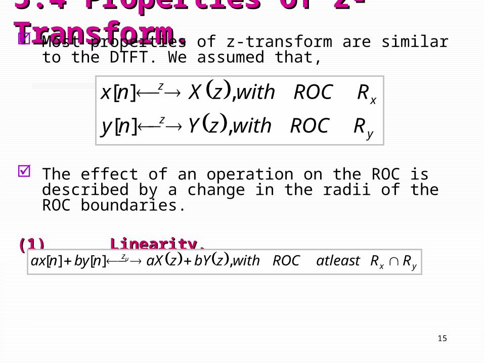
5.4 Properties of z-5.4 Properties of z-Transform.Transform. Most properties of z-transform are similar to the

DTFT. We assumed that,

The effect of an operation on the ROC is described by a change in the radii of the ROC boundaries.

(1)(1) Linearity, Linearity,

y

z

xz

RROCwithzYny

RROCwithzXnx

,][

,][

yxz RRatleastROCwithzbYzaXnbynax u ,][][

16

(2) Time Reversal.(2) Time Reversal.

(3) Time Shift.(3) Time Shift.

with ROC Rx, except possibly z=0 or |z|= infinity.

zXznnx nz 0][ 0

.1

,1

][x

z

RROCwith

zXnx

Cont’d…Cont’d…

17

(4) Multiplication by an Exponential (4) Multiplication by an Exponential Sequence.Sequence.

(5) Convolution.(5) Convolution.

(6) Differentiation in the z-Domain.(6) Differentiation in the z-Domain.

xzn RROCwith

a

zXnx ||,][

yxz RRatleastROCwithzYzXnynx ,][*][

xz RROCwithzX

dz

dznnx ,,][

Cont’d…Cont’d…

18

There are two common methods;

5.5.1 Partial-Fraction Expression.5.5.1 Partial-Fraction Expression.

5.5.2 Power-Series Expansion.5.5.2 Power-Series Expansion.

5.5 The Inverse Z-5.5 The Inverse Z-Transform.Transform.

19

5.5.1 Partial-Fraction 5.5.1 Partial-Fraction Expansion.Expansion.Example 5.1:Example 5.1: Inversion by Partial-Fraction Inversion by Partial-Fraction

Expansion.Expansion.Find the inverse z-transform of,

with ROC 1<|z|<2.

Figure 5.6: Locations of poles and ROC.Figure 5.6: Locations of poles and ROC.

Solution:Solution:

Step 1Step 1:: Use the partial fraction expansion of Z(Use the partial fraction expansion of Z(ss) ) to writeto write

Solving the A, B and C will give

)1)(21)(2

11(

1)(

111

21

zzz

zzzX

)1(

2

)21(

2

)2

11(

1)(

111

zzz

zX

)1()21()2

11(

)(11

1

z

C

z

B

z

AzX

20

Step 2Step 2:: Find the Inverse z-Transform for each Find the Inverse z-Transform for each Terms.Terms.

- The ROC has a radius greater than the pole at z=1/2, it is the right-sided inverse z-transform.

- The ROC has a radius less than the pole at z=2, it is the left-sided inverse z-transform.

- Finally the ROC has a radius greater than the pole at z=1, it is the right-sided inverse z-transform.

)2

11(

1][

2

1

1

znu z

n

)21(

2]1[)2(2

1

znu zn

)1(

2][2

1

znu z

Cont’d…Cont’d…

21

Step 3Step 3: : Combining the Terms.Combining the Terms.

.

].[2]1[)2(2][2

1][ nunununx n

n

)1(

2

)21(

2

)2

11(

1)(

111

zzz

zX

Cont’d…Cont’d…

22

Example 5.2:Example 5.2: Inversion of Improper Inversion of Improper Rational Function.Rational Function.Find the inverse z-transform of,

with ROC |z|<1.

Figure 5.7: Locations of poles and ROC.Figure 5.7: Locations of poles and ROC.

Solution:Solution:

Step 1Step 1:: Convert Convert XX((zz) into Ratio of Polynomial in z) into Ratio of Polynomial in z--

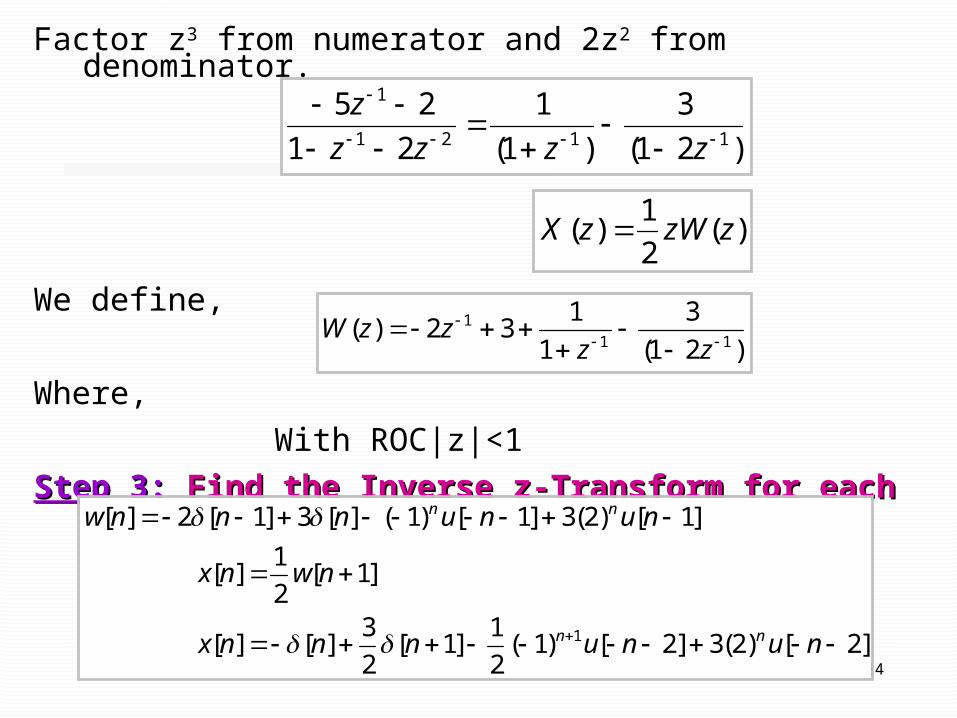
11..Factor z3 from numerator and 2z2 from denominator.

422

4410)(

2

23

zz

zzzzX

21

321

2

3

21

44101

2)(

zz

zzz

z

zzX

21

321

21

44101

2)(

zz

zzzzzX

23

Step 2Step 2: Use long division to reduce order of : Use long division to reduce order of numerator polynomial.numerator polynomial.

Factor z3 from numerator and 2z2 from denominator.

)21)(1(

2532

21

2532

21

44101

11

11

21

11

21

321

zz

zz

zz

zz

zz

zzz

25

336

186

224

__________32

1104412

1

12

12

123

1

12312

z

zz

zz

zzz

z

zzzzz

24

Factor z3 from numerator and 2z2 from denominator.

We define,

Where,

With ROC|z|<1

Step 3Step 3:: Find the Inverse z-Transform for each Find the Inverse z-Transform for each Terms.Terms.

.

)21(

3

)1(

1

21

251121

1

zzzz

z

)(2

1)( zzWzX

)21(

3

1

132)(

111

zzzzW

]2[)2(3]2[)1(2

1]1[

2

3][][

]1[2

1][

]1[)2(3]1[)1(][3]1[2][

1

nununnnx

nwnx

nununnnw

nn

nn

25

5.6 Transfer Function.5.6 Transfer Function. The transfer function is defined as the z-transform

of the impulse response. y[n]= h[n]*x[n] Take the z-transform of both sides of the equation

and use the convolution properties result in,

Rearrange the above equation result in the ratio of the z-transform of the output signal to the z-transform of the input signal.

The definition applies at all z in the ROC of X(z) and Y(z) for which X(z) is nonzero.

)()()( zXzHzY

)(

)()(

zX

zYzH

26

Example 5.3:Example 5.3: Find the Transfer Function.Find the Transfer Function.Find the transfer function and the impulse response of a causal LTI system if the input to the system is

Solution:Solution:

Step 1Step 1:: Find the z-Transform of the input X(z) and output Find the z-Transform of the input X(z) and output Y(z).Y(z).

With ROC |z|>1/3

With ROC |z|>1.

1

3

11

1)(

z

zX

].[3

1][)1(3][

,][3

1][

nununy

outputandnunx

nn

n

)3

11)(1(

4

)3

11(

1

)1(

3)(

11

11

zz

zzzY

27

Step 2Step 2: : Solve for H(z).Solve for H(z).

, with ROC |z|>1.

Solve for impulse response h[n],

, with ROC |z|>1.

So the impulse response h[n] is,

.

11

1

3

11)1(

3

114

)(

zz

z

zH

].[)3/1(2][)1(2][ nununh nn

1

1

3

11

2

)1(

2)(

zz

zH

28

5.7 Causality and 5.7 Causality and Stability.Stability. The impulse response of a causal system is zero

for n<0. The impulse response of a casual LTI system is

determined from the transfer function by using right-sided inverse transform.

The poles inside the unit circle, contributes an exponentially decaying term to the impulse response.

The poles outside the unit circle, contributes an exponentially increasing term.

Figure 5.8: Pole and impulse Figure 5.8: Pole and impulse response characteristic of a response characteristic of a causal system. causal system. (a) A pole inside the unit circle (a) A pole inside the unit circle contributes an exponentially contributes an exponentially decaying term to the impulse decaying term to the impulse response. response. (b) A pole outside the unit circle (b) A pole outside the unit circle contributes an exponentially contributes an exponentially increasing term to the impulse increasing term to the impulse response.response.

29

Stable system; the impulse response is absolute summable and the DTFT of impulse response exist.

The impulse response of a casual LTI system is determined from the transfer function by using right-sided inverse transform.

The poles inside the unit circle, contributes a right-sided decaying exponential term to the impulse response.

The poles outside the unit circle, contributes a left-sided decaying exponentially term to the impulse response.

Refer to Figure 5.9.

Figure 5.9: Pole and impulse Figure 5.9: Pole and impulse response characteristics for a response characteristics for a stable system. stable system. (a) A pole inside the unit circle (a) A pole inside the unit circle contributes a right-sided term to contributes a right-sided term to the impulse response. (b) A pole the impulse response. (b) A pole outside the unit circle outside the unit circle contributes a left-sided term to contributes a left-sided term to the impulse response.the impulse response.

Cont’d…Cont’d…

30

From the ROC below the system is stable, because all the poles within the unit circle and causal because the right-sided decaying exponential in terms of impulse response.

Figure 7.16: A system that is both stable and causal must Figure 7.16: A system that is both stable and causal must have all its poles inside the unit circle in the have all its poles inside the unit circle in the zz-plane, as -plane, as

illustrated here.illustrated here.

Stable/Stable/Causal ?Causal ?

Cont’d…Cont’d…

31

5.8 Implementing 5.8 Implementing Discrete-Time LTI Discrete-Time LTI System.System. The system is represented by the differential

equation.

Taking the z-transform of difference equation gives,

The transfer function of the system,

]2[]1[][]2[]1[][ 21021 nxbnxbnxbnyanyany

)()()()1( 22

110

22

11 zXzbzbbzYzaza

22

11

22

110

1)(

)(

)()(

zaza

zbzbbzH

zX

zYzH

32

Example 5.4 :Example 5.4 : Causality and Stability.Causality and Stability.

Can this system be both stable and causal?

Solution:Solution:Step 1Step 1:: Find the characteristic equation of the Find the characteristic equation of the

system.system.

From the plot, the system is unstable

because the pole at z = 1.2 is outside

the unit circle.

.

33

Figure 7.26: Block diagram of the transfer function.Figure 7.26: Block diagram of the transfer function.

)()()()1( 22

110

22

11 zXzbzbbzYzaza

Cont’d…Cont’d…

34

Figure 7.27: Development of the direct form II representation of Figure 7.27: Development of the direct form II representation of an LTI system. (a) Representation of the transfer function an LTI system. (a) Representation of the transfer function HH((zz) )

as as HH22((zz))HH11((zz). ). (b) Direct form II implementation of the transfer function (b) Direct form II implementation of the transfer function HH((zz) )

obtained from (a) by collapsing the two sets of obtained from (a) by collapsing the two sets of zz–1–1 blocks. blocks.

Cont’d…Cont’d…

35

5.9 The Unilateral z-5.9 The Unilateral z-Transform.Transform. The unilateral z-Transform of a signal x[n] is

defined as,

Properties. If two causal DT signals form these transform

pairs,

(1) Linearity.

(2) Time Shifting.

X z x n z nn0

g n Z G z and h n Z H z

g n h n Z G z H z

g n n0 Z z n0 G z , n0 0

g n n0 Z zn0 G z g m z mm0

n0 1

, n0 0