Full-Scale Unsteady RANS CFD Simulations of Ship Behaviour and Performance in Head Seas due to Slow Steaming Tahsin Tezdogan * , Yigit Kemal Demirel, Paula Kellett, Mahdi Khorasanchi, Atilla Incecik, Osman Turan Department of Naval Architecture, Ocean and Marine Engineering, Henry Dyer Building, University of Strathclyde, 100 Montrose Street, Glasgow, G4 0LZ, UK * corresponding author; e-mail: [email protected], phone: +44(0)1415484912 ABSTRACT It is critical to be able to estimate a ship’s response to waves, since the resulting added resistance and loss of speed may cause delays or course alterations, with consequent financial repercussions. Slow steaming has recently become a popular approach for commercial vessels, as a way of reducing fuel consumption, and therefore operating costs, in the current economic and regulatory climate. Traditional methods for the study of ship motions are based on potential flow theory and cannot incorporate viscous effects. Fortunately, unsteady Reynolds-Averaged Navier-Stokes computations are capable of incorporating both viscous and rotational effects in the flow and free surface waves. The key objective of this study is to perform a fully nonlinear unsteady RANS simulation to predict the ship motions and added resistance of a full scale KRISO Container Ship model, and to estimate the increase in effective power and fuel consumption due to its operation in waves. The analyses are performed at design and slow steaming speeds, covering a range of regular head waves, using a commercial RANS solver. The results are validated against available experimental data and are found to be in good agreement with the experiments. Also, the results are compared to those from potential theory. 1
Transcript
Full-Scale Unsteady RANS CFD Simulations of Ship Behaviour and Performance in Head Seas due to Slow Steaming
Tahsin Tezdogan*, Yigit Kemal Demirel, Paula Kellett, Mahdi Khorasanchi, Atilla Incecik, Osman Turan
Department of Naval Architecture, Ocean and Marine Engineering, Henry Dyer Building, University of Strathclyde, 100 Montrose Street, Glasgow, G4 0LZ, UK
It is critical to be able to estimate a ship’s response to waves, since the resulting added resistance and loss of speed may cause delays or course alterations, with consequent financial repercussions. Slow steaming has recently become a popular approach for commercial vessels, as a way of reducing fuel consumption, and therefore operating costs, in the current economic and regulatory climate. Traditional methods for the study of ship motions are based on potential flow theory and cannot incorporate viscous effects. Fortunately, unsteady Reynolds-Averaged Navier-Stokes computations are capable of incorporating both viscous and rotational effects in the flow and free surface waves. The key objective of this study is to perform a fully nonlinear unsteady RANS simulation to predict the ship motions and added resistance of a full scale KRISO Container Ship model, and to estimate the increase in effective power and fuel consumption due to its operation in waves. The analyses are performed at design and slow steaming speeds, covering a range of regular head waves, using a commercial RANS solver. The results are validated against available experimental data and are found to be in good agreement with the experiments. Also, the results are compared to those from potential theory.
1.0 IntroductionUnderstanding the behaviour of a vessel in a real seaway is critical for determining its performance. Rough sea conditions induce significant ship motions, which affect a ship’s resistance. The resulting increase in resistance can compromise propulsive efficiency and can increase fuel consumption. Ship motions and seakeeping behaviour are also very important with regards to crew, vessel and cargo safety. An awareness of the impacts of ship motions on resistance is particularly important in the current economic climate, which has seen a significant increase in fuel costs in comparison to charter rates. For example, for a typical commercial vessel, the fuel costs will now account for well over half of its operating costs, whereas for a container ship, the figure may be as high as 75% (Ronen, 2011).
The current economic climate is very different from the “boom years” in which modern vessels were designed. In response to recent fuel price increases, ship operators have begun to apply the slow steaming approach, which was initially proposed by Maersk technical experts post-2007 (Maersk, n.d.). In this approach, a vessel is operated at a speed significantly below
1
its original design speed in order to reduce the amount of fuel that is required. Slow steaming is typically defined as being down to around 18 knots for container vessels, with operational speeds below this being termed ‘super slow steaming’. Figure 1 below, taken from Banks et al. (2013), shows how the operating speeds for container vessels have decreased over recent years, comparing the period from 2006-2008 with 2009-2012. It can be seen that a typical operating speed is now significantly below the original design speeds which would have been specified for these vessels. In particular, it can be observed that for this collection of data, the most typical slow steaming speed is around 19 knots. This speed will therefore be used as a representative slow steaming speed in this study.
Figure 1- Comparison of the speed distributions for container vessels, taken from Banks et al. (2013).
Other concepts such as “just-in-time” operation and virtual arrival are also applied as a means of reducing speed without compromising the agreed dates for charter cargo delivery into port. In some cases, vessels are even retro-fitted with lower power propulsion systems to reduce weight and improve efficiency, as well as reduce the problems which may arise from the long-term operation of machinery in off-design conditions. However, little research has been carried out into the effect that these lower speeds may have on the behaviour of the vessel, and whether further fuel savings may be an additional benefit. This paper addresses the gap in current knowledge by comparing pitch and heave motions, as well as added resistance, at both design and slow steaming speeds. More importantly, although extensive research has been performed to investigate increases in effective power, ship fuel consumption and CO2
emissions, no specific study exists which aims to predict the increase in the above mentioned parameters due to the operation in waves, using a Computational Fluid Dynamics (CFD)-based Reynolds Averaged Navier-Stokes (RANS) approach. Therefore, the main aim of this study is to directly predict the increase in the required effective power of a vessel operating in regular head seas. This leads to a rough estimation of the fuel penalty to counter the additional CO2 emissions from the vessel. The potential benefits of slow steaming will be probed by invoking added resistance predictions.
The Energy Efficiency Operational Indicator (EEOI) was introduced by the International Maritime Organisation (IMO) in 2009 as a voluntary method for monitoring the operational performance of a ship. The EEOI enables an assessment to be made of the operational energy efficiency of a ship, which is expressed in terms of the CO2 emitted per unit of transport work (Organisation, 2009). Alongside this, regulations relating to the control of SOx emissions
2
from shipping were introduced, with specific limits stipulated. This will be followed by limits for NOx emissions in 2016, with limits for CO2 and particulate matter (PM) emissions also likely to be introduced in the future. Reducing the fuel consumption through slow steaming, and improving or at least maintaining propulsive efficiency, will take steps towards addressing these requirements.
The resistance of a ship operating in a seaway is greater than its resistance in calm water. The difference between these two resistances arises from ship motions and wave drift forces in waves and has been termed the added resistance due to waves. Added resistance can account for up to 15-30% of the total resistance in calm water (Arribas, 2007). It is therefore critical to be able to accurately predict the added resistance of a ship in waves, and this should be included in ship performance assessments. One purpose of this study is to predict the added resistance due to waves with higher accuracy than potential theory-based methods.
The KRISO Container Ship (KCS), developed by the Korean Maritime and Ocean Engineering Research Institute (now MOERI), has been used in a wide range of research studies. There is consequently a wide range of experimental and simulation data available for comparison, and for verification and validation purposes. The KCS has therefore been investigated in this study due to the ready availability of this data and research in the public domain. Moreover, container ships are particularly affected by slow steaming, as they were designed to operate with very high design speeds, in the region of up to 25 knots. The service speed for KCS is 24 knots. This makes the KCS model particularly relevant for this study.
As discussed by the International Towing Tank Conference (ITTC) (2011b), advances in numerical modelling methods and increases in computational power have made it possible to carry out fully non-linear simulations of ship motions, taking into account viscous effects, using CFD. In this study, an unsteady RANS approach is applied using the commercial CFD software Star-CCM+ version 9.0.2, which was developed by CD-Adapco. Additionally, the supercomputer facilities at the University of Strathclyde have been utilised to allow much faster and more complex simulations.
A full-scale KCS hull model appended with a rudder is used for all simulations, to avoid scaling effects. The model was first run in calm water conditions free to trim and sink so that the basic resistance could be obtained, for both the design and the slow steaming speeds. The model was then run in a seaway, to allow the ship motions to be observed and to allow the added resistance due to waves to be calculated. This was again carried out for both speeds in question. The resistance was monitored as a drag force on the hull, and the pitch and heave time histories were recorded.
This paper is organised as follows. Section 2 gives a brief literature review on seakeeping methods and the implementation of RANS methods for the solution of seakeeping problems. Afterwards, the main ship properties are given, and a list of the simulation cases applied to the current CFD model is introduced in detail in Section 3. Next, in Section 4, the numerical setup of the CFD model is explained, with details provided in the contained sub-sections. Following this, all of the results from this work, including validation and verification studies, are demonstrated and discussed in Section 5. Finally, in Section 6, the main results drawn from this study are briefly summarised, and suggestions are made for future research.
2.0 BackgroundThe vast majority of the available techniques to predict ship motions, as well as the added resistance due to waves, rely on assumptions from potential flow theory, including free surface effects. However, many previous studies such as Schmitke (1978) have shown that
3
viscous effects are likely to be the most significant, particularly in high amplitude waves and at high Froude numbers.
Beck and Reed (2001) estimate that in the early 2000s, 80% of all seakeeping computations at forward speeds were performed using strip theory, owing to its fast solutions. Another advantage of strip theory is that it is applicable to most conventional ship geometries. On the other hand, as discussed by Newman (1978), the conventional strip theories are subject to some deficiencies in long incident waves and at high Froude numbers. This is thought to be caused by the evolution of forward speed effects and the complex nature of the diffraction problem. Faltinsen and Zhao (1991) also state that strip theory is questionable when applied at high speeds, since it accounts for the forward speed in a simplistic manner. Discrepancies between strip theory and experiments for higher speed vessels, or highly non-wall sided hull forms, have therefore motivated research to develop more advanced theories, such as the 3-D Rankine panel method, unsteady RANS methods and Large Eddy Simulation (LES) methods (Beck and Reed, 2001).
As computational facilities become more powerful and more accessible, the use of 3-D techniques to study seakeeping problems is becoming more common. As explained in detail by Tezdogan et al. (2014b), Yasukawa (2003) claims that 3-D methods have been developed to overcome the deficiencies in the strip theory methods. In the method developed by Bertram and Yasukawa (1996), full 3-D effects of the flow and forward speed are accounted for, in contrast to strip theory where these effects are not properly taken into account. Yasukawa (2003) applied the theory of Bertram and Yasukawa (1996) to several container carriers with strong flare. As a result of his study, it was reported that hydrodynamic forces, ship motions and local pressures are much better predicted using the theory of Bertram and Yasukawa (1996) than the results obtained by strip theory when compared to experiments. However, the predicted lateral hydrodynamic forces are not satisfactory, due to the viscous flow effect. Yasukawa (2003) suggests that this problem can be diminished by applying empirical corrections, similar to those employed in strip theory.
Simonsen et al. (2013) highlight that the effects which are ignored in the potential theory such as breaking waves, turbulence and viscosity should be directly taken into account in the numerical methods. RANS methods, for instance, are very good alternatives to the potential flow theory as they can directly incorporate viscous effects in their equations.
Continued technological advances offer ever-increasing computational power. This can be utilised for viscous flow simulations to solve RANS equations in the time domain. CFD-based RANS methods are rapidly gaining popularity for seakeeping applications. These methods have the distinct advantage of allowing designers to assess the seakeeping performance of a vessel during the design stages, therefore allowing any corrective action to be taken promptly, before the vessel is actually built (Tezdogan et al., 2014a).
In 1994, a CFD workshop was organised in Tokyo to discuss the implementation of steady RANS methods to provide a solution for free-surface flows around surface ships. As explained by Wilson et al. (1998), from that point onwards, RANS methods have been widely used in many marine hydrodynamics applications.
As discussed by Simonsen et al. (2013), RANS-based CFD methods have been used extensively for seakeeping performance analyses with several ship types, by many scholars. Sato et al. (1999) conducted CFD simulations to predict motions of the Wigley hull and Series 60 models in head seas. Hochbaum and Vogt (2002) then performed simulations of a C-Box container ship in 3 degrees-of-freedom motions (surge, heave and pitch) in head seas. Following this, Orihara and Miyata (2003) predicted the added resistance and pitch and heave
4
responses of the S-175 container ship in regular head seas, using the Baldwin-Lomax turbulence model. In their work, they investigated the effect of two selected bulbous forms on the predicted added resistance.
CFD simulations have been also performed for more complex ship geometries. Weymouth et al. (2005), for example, simulated the pitch and heave motions of a Wigley hull in regular incoming waves. Carrica et al. (2007) studied the motions of a DTMB 5512 model in regular, small amplitude head waves. Hu and Kashiwagi (2007) also investigated the pitch and heave responses of a Wigley hull in head seas. Stern et al. (2008) studied the pitch and heave responses of BIW-SWATH in regular head waves. Wilson et al. (2008) and Paik et al. (2009) performed CFD simulations to predict the pitch and heave transfer functions of the S-175 ship in regular head waves. Carrica et al. (2008) demonstrated an application of an unsteady RANS CFD method to simulate a broaching event for an auto-piloted ONR Tumblehome in both regular and irregular seas. Then, Castiglione et al. (2011) investigated the motion responses of a high speed DELFT catamaran in regular head waves at three different speeds. Following this, Castiglione et al. (2013) carried out CFD simulations for seakeeping of the same catamaran model at two Froude numbers in both head and oblique regular waves.
Bhushan et al. (2009) performed resistance and powering computations of the full-scale self-propelled Athena ship free to sink and trim using both smooth and rough wall functions. They also carried out seakeeping simulations at both full and model scale along with manoeuvring calculations for DTMB 5415 at full-scale. Mousaviraad et al. (2010) obtained heave and pitch response amplitudes and phases of the DTMB 5512 model in head seas using regular wave and transient wave group procedures. Following this, Simonsen and Stern (2010) performed CFD RANS simulations to obtain the heave and pitch motions and added resistance for the KCS model, presenting it at the Gothenburg 2010 CFD workshop. In addition, Enger et al. (2010) contributed to the same workshop with their study on the dynamic trim, sinkage and resistance analyses of the model KCS by using the Star-CCM+ software package. In their work, it was demonstrated that the CFD results agreed well with the experimental results.
Following this, Carrica et al. (2011) presented two computations of KCS in model scale, utilising CFDShip-Iowa, which is a general-purpose CFD simulation software developed at the University of Iowa. They performed self-propulsion free to sink and trim simulations in calm water, followed by pitch and heave simulations in regular head waves, covering three conditions at two different Froude numbers (Fn=0.26 and 0.33). Then, Kim (2011) carried out CFD analyses for a 6500 TEU container carrier, focusing on the global ship motions and structural loads by successfully validating the results against the model test measurements. After the validation study, Kim (2011) claimed that the current CFD technology would facilitate the decision making process in ship optimisation. Finally, Simonsen et al. (2013) investigated motions, flow field and resistance for an appended KCS model in calm water and regular head seas by means of Experimental Fluid Dynamics (EFD) and CFD. They focused mainly on large amplitude motions, and hence studied the near resonance and maximum excitation conditions. The results obtained using the CFD methods were compared to those from their experiments and the potential flow theory method.
To the best of our knowledge, the majority of RANS seakeeping simulations have been performed at model scale. However, as Hochkirch and Mallol (2013) claim, model-scale flows and full-scale flows can show significant differences due to scale effects. They explain that the discrepancies between model and full scale mainly stem from relatively different boundary layers, flow separation, and wave breaking, particularly behind transom sterns. Visonneau et al. (2006) draw a conclusion in their paper that, “[…] complete analysis of the scale effects on free-surface and of the structure of the viscous stern flow reveals that these
5
scale effects are not negligible and depend strongly on the stern geometries”. As discussed in detail with several examples by Hochkirch and Mallol (2013), performing analyses at a full scale is of the greatest importance, especially for hulls appended with propulsion improving devices (PIDs). A decision was therefore made to use the full-scale KCS model in the CFD simulations presented in this paper.
In addition, during this literature review, it was seen that when using the KCS model, although resistance predictions have been conducted for a range of Froude numbers (for example (J.B. Banks et al., 2010), (Enger et al., 2010)), seakeeping analyses have only been performed at forward speeds corresponding to a Froude number of 0.26 or higher (for example (Simonsen et al., 2013), (P. M. Carrica et al., 2011)). This study therefore may be useful to understand the seakeeping behaviour and performance of the KCS model at a slow steaming speed.
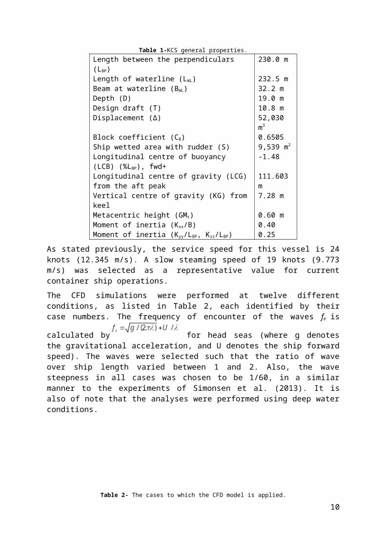
3.0 Ship Geometry and ConditionsA full scale model of the KCS appended with a rudder was used within this study. The main properties of the KCS model are presented in Table 1 (Kim et al., 2001):
Table 1-KCS general properties.Length between the perpendiculars (LBP) 230.0 mLength of waterline (LWL) 232.5 mBeam at waterline (BWL) 32.2 mDepth (D) 19.0 mDesign draft (T) 10.8 mDisplacement (Δ) 52,030 m3
Block coefficient (CB) 0.6505Ship wetted area with rudder (S) 9,539 m2
Longitudinal centre of buoyancy (LCB) (%LBP), fwd+ -1.48Longitudinal centre of gravity (LCG) from the aft peak 111.603 mVertical centre of gravity (KG) from keel 7.28 mMetacentric height (GMt) 0.60 mMoment of inertia (Kxx/B) 0.40Moment of inertia (Kyy/LBP, Kzz/LBP) 0.25
As stated previously, the service speed for this vessel is 24 knots (12.345 m/s). A slow steaming speed of 19 knots (9.773 m/s) was selected as a representative value for current container ship operations.
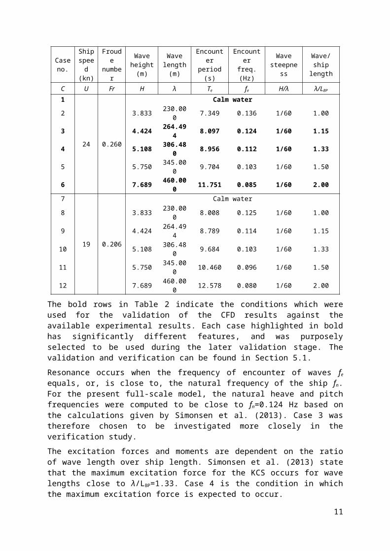
The CFD simulations were performed at twelve different conditions, as listed in Table 2, each identified by their case numbers. The frequency of encounter of the waves fe is calculated by
for head seas (where g denotes the gravitational acceleration, and U denotes the ship forward speed). The waves were selected such that the ratio of wave over ship length varied between 1 and 2. Also, the wave steepness in all cases was chosen to be 1/60, in a similar manner to the experiments of Simonsen et al. (2013). It is also of note that the analyses were performed using deep water conditions.
6
Table 2- The cases to which the CFD model is applied.
The bold rows in Table 2 indicate the conditions which were used for the validation of the CFD results against the available experimental results. Each case highlighted in bold has significantly different features, and was purposely selected to be used during the later validation stage. The validation and verification can be found in Section 5.1.
Resonance occurs when the frequency of encounter of waves fe equals, or, is close to, the natural frequency of the ship fn. For the present full-scale model, the natural heave and pitch frequencies were computed to be close to fn=0.124 Hz based on the calculations given by Simonsen et al. (2013). Case 3 was therefore chosen to be investigated more closely in the verification study.
The excitation forces and moments are dependent on the ratio of wave length over ship length. Simonsen et al. (2013) state that the maximum excitation force for the KCS occurs for wave lengths close to λ/LBP=1.33. Case 4 is the condition in which the maximum excitation force is expected to occur.
Case 6, according to the work by Carrica et al. (2011), exhibits a very linear behaviour since the wavelength is very large. It can hence be regarded as the most linear condition amongst all of the cases.
4.0 Numerical ModellingUp to this point, this paper has provided a background to this study and has given an introduction to the work. The following section will provide details of the numerical simulation approaches used in this study and will discuss the numerical methods applied to the current CFD model.
4.1 Governing equationsFor incompressible flows without body forces, the averaged continuity and momentum equations may be written in tensor form and Cartesian coordinates as follows (Ferziger and Peric, 2002):
7
(1)
(2)
in which ij are the mean viscous stress tensor components, as shown in Eq. 3
(3)
and p is the mean pressure, is the averaged Cartesian components of the velocity vector,
is the Reynolds stresses, ρ is the fluid density and μ is the dynamic viscosity.
To model fluid flow, the solver employed uses a finite volume method which discretises the integral formulation of the Navier-Stokes equations. The RANS solver employs a predictor-corrector approach to link the continuity and momentum equations.
4.2 Physics modellingThe turbulence model selected in this study was a standard k-ε model, which has been extensively used for industrial applications (CD-Adapco, 2014). Also, Querard et al. (2008) note that the k-ε model is quite economical in terms of CPU time, compared to, for example, the SST turbulence model, which increases the required CPU time by nearly 25%. The k-ε turbulence model has also been used in many other studies performed in the same area, such as Kim and Lee (2011) and Enger et al. (2010).
The “Volume of Fluid” (VOF) method was used to model and position the free surface, either with a flat or regular wave. CD-Adapco (2014) defines the VOF method as, “a simple multiphase model that is well suited to simulating flows of several immiscible fluids on numerical grids capable of resolving the interface between the mixture’s phases”. Because it demonstrates high numerical efficiency, this model is suitable for simulating flows in which each phase forms a large structure, with a low overall contact area between the different phases. One example of such flow is the sloshing of water in a tank, during which the free surface remains perpetually smooth. If the movement of the tank becomes stronger, then breaking waves, air bubbles in the water and airborne water droplets will form as a result. The VOF model uses the assumption that the same basic governing equations as those used for a single phase problem can be solved for all the fluid phases present within the domain, as it is assumed that they will have the same velocity, pressure and temperature. This means that the equations are solved for an equivalent fluid whose properties represent the different phases and their respective volume fractions (CD-Adapco, 2014). The inlet velocity and the volume fraction of both phases in each cell, as well as the outlet pressure, are all functions of the flat wave or regular wave used to simulate the free surface. The free surface is not fixed; it is dependent on the specifications of this flat or regular wave, with the VOF model making calculations for both the water and air phases. The grid is simply refined in order to enable the variations in volume fraction to be more accurately captured. In this work, a second-order convection scheme was used throughout all simulations in order to accurately capture sharp interfaces between the phases.
8
Figure 2 demonstrates how the free surface was represented in this CFD model by displaying the water volume fraction profile on the hull. In the figure, for instance, a value of 0.5 for the volume fraction of water implies that a computational cell is filled with 50% water and 50% air. This value therefore indicates the position of the water-air interface, which corresponds to the free surface.
Figure 2– Free surface representation on the ship hull.
It should also be mentioned that in the RANS solver, the segregated flow model, which solves the flow equation in an uncoupled manner, was applied throughout all simulations in this work. Convection terms in the RANS formulae were discretised by applying a second-order upwind scheme. The overall solution procedure was obtained according to a SIMPLE-type algorithm.
In order to simulate realistic ship behaviour, a Dynamic Fluid Body Interaction (DFBI) model was used with the vessel free to move in the pitch and heave directions. The DFBI model enabled the RANS solver to calculate the exciting force and moments acting on the ship hull due to waves, and to solve the governing equations of rigid body motion in order to re-position the rigid body (CD-Adapco, 2014).
4.2.1 Choice of the time step
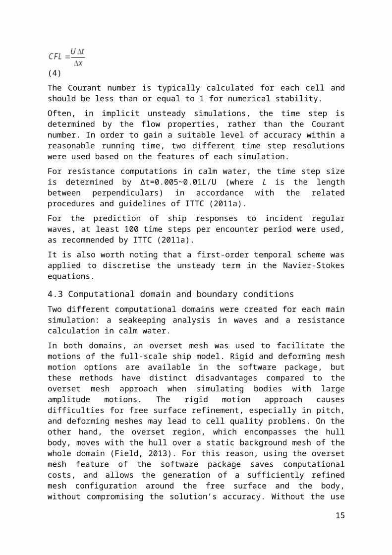
The Courant number (CFL), which is the ratio of the physical time step (Δt) to the mesh convection time scale, relates the mesh cell dimension Δx to the mesh flow speed U as given below:
(4)
The Courant number is typically calculated for each cell and should be less than or equal to 1 for numerical stability.
Often, in implicit unsteady simulations, the time step is determined by the flow properties, rather than the Courant number. In order to gain a suitable level of accuracy within a reasonable running time, two different time step resolutions were used based on the features of each simulation.
For resistance computations in calm water, the time step size is determined by Δt=0.005~0.01L/U (where L is the length between perpendiculars) in accordance with the related procedures and guidelines of ITTC (2011a).
For the prediction of ship responses to incident regular waves, at least 100 time steps per encounter period were used, as recommended by ITTC (2011a).
9
It is also worth noting that a first-order temporal scheme was applied to discretise the unsteady term in the Navier-Stokes equations.
4.3 Computational domain and boundary conditionsTwo different computational domains were created for each main simulation: a seakeeping analysis in waves and a resistance calculation in calm water.
In both domains, an overset mesh was used to facilitate the motions of the full-scale ship model. Rigid and deforming mesh motion options are available in the software package, but these methods have distinct disadvantages compared to the overset mesh approach when simulating bodies with large amplitude motions. The rigid motion approach causes difficulties for free surface refinement, especially in pitch, and deforming meshes may lead to cell quality problems. On the other hand, the overset region, which encompasses the hull body, moves with the hull over a static background mesh of the whole domain (Field, 2013). For this reason, using the overset mesh feature of the software package saves computational costs, and allows the generation of a sufficiently refined mesh configuration around the free surface and the body, without compromising the solution’s accuracy. Without the use of the overset mesh feature, simulating a full-scale ship model in waves would require a very high cell number, requiring much more computational power.
In all CFD problems, the initial conditions and boundary conditions must be defined depending on the features of the problem to be solved. The determination of these boundary conditions is of critical importance in order to be able to obtain accurate solutions. There are a vast number of boundary condition combinations that can be used to approach a problem. However, the selection of the most appropriate boundary conditions can prevent unnecessary computational costs when solving the problem (Date and Turnock, 1999).
When using the overset mesh feature, two different regions were created to simulate ship responses in waves, namely background and overset regions. A general view of the computation domain with the KCS hull model and the notations of selected boundary conditions are depicted in Figure 3.
In order to reduce computational complexity and demand, only half of the hull (the starboard side) is represented. A symmetry plane forms the centreline domain face in order to accurately simulate the other half of the model. It should be noted that in some figures given hereafter, the mirror image of the ship and domain is reflected on the port side for plotting purposes.
10
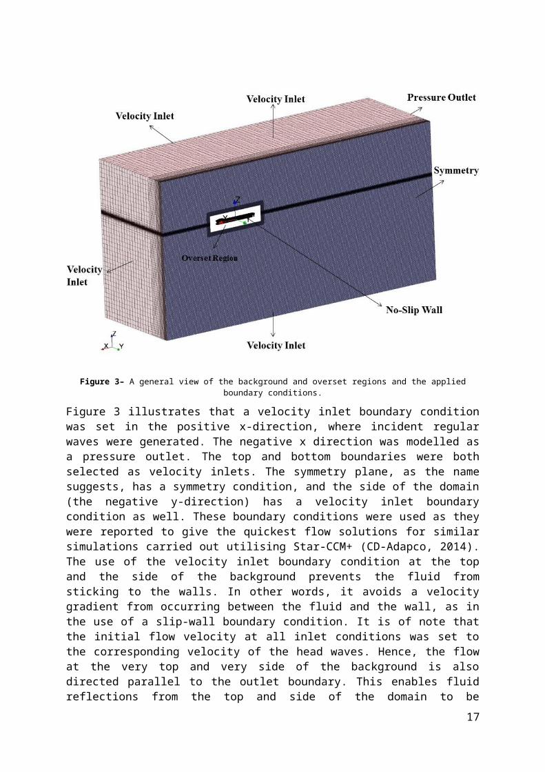
Figure 3– A general view of the background and overset regions and the applied boundary conditions.
Figure 3 illustrates that a velocity inlet boundary condition was set in the positive x-direction, where incident regular waves were generated. The negative x direction was modelled as a pressure outlet. The top and bottom boundaries were both selected as velocity inlets. The symmetry plane, as the name suggests, has a symmetry condition, and the side of the domain (the negative y-direction) has a velocity inlet boundary condition as well. These boundary conditions were used as they were reported to give the quickest flow solutions for similar simulations carried out utilising Star-CCM+ (CD-Adapco, 2014). The use of the velocity inlet boundary condition at the top and the side of the background prevents the fluid from sticking to the walls. In other words, it avoids a velocity gradient from occurring between the fluid and the wall, as in the use of a slip-wall boundary condition. It is of note that the initial flow velocity at all inlet conditions was set to the corresponding velocity of the head waves. Hence, the flow at the very top and very side of the background is also directed parallel to the outlet boundary. This enables fluid reflections from the top and side of the domain to be prevented. In addition to this, the selection of the velocity inlet boundary condition for the top and bottom facilitate the representation of the deep water and infinite air condition, which is also the case in open seas. The top, bottom and side boundaries could have been set as a slip-wall or symmetry plane. The selection of boundary conditions from any appropriate combination would not affect the flow results significantly, provided that they are placed far enough away from the ship hull, such that the flow is not disturbed by the presence of the body. Also, the pressure outlet boundary condition was set behind the ship since it prevents backflow from occurring and fixes static pressure at the outlet.
Date and Turnock (1999) point out that, just as the selection of the boundaries is of great importance, their positioning is equally important. It has to be ensured that no boundaries have an influence on the flow solution.
11
ITTC (2011a) recommends that for simulations in the presence of incident waves, the inlet boundary should be located 1-2LBP away from the hull, whereas the outlet should be positioned 3-5LBP downstream to avoid any wave reflection from the boundary walls. Three other pieces of previous work similar to this study have also been consulted to decide the locations of the boundaries. The findings are summarised in Table 3.
Table 3– The locations of the boundaries in similar previous studies.Directions
Reference Upstream Downstream Up Bottom TransverseShen and Wan (2013) 1LBP 4LBP 1LBP 1LBP 1.5LBP
Ozdemir et al. (2014) 2LBP 3LBP 2LBP 2LBP 2LBP
Simonsen et al. (2013) 0.6LBP 2LBP N/A N/A 1.5LBP
The locations of the boundaries are illustrated in Figure 4, which gives front and side views of the domain. It is worth mentioning that throughout all the cases, in order to prevent wave reflection from the walls, the VOF wave damping capability of the software package was applied to the background region with a damping length equal to 1.24LBP (~285 m.). This numerical beach model was used in downstream, bottom and transverse directions.
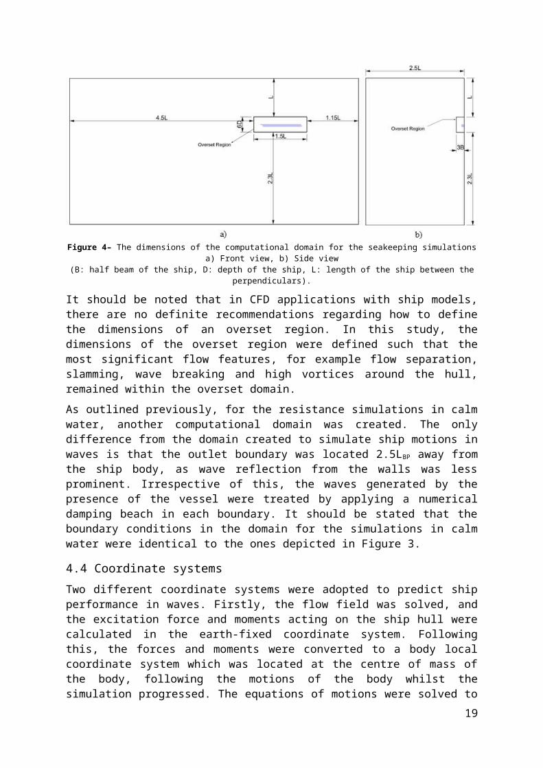
Figure 4– The dimensions of the computational domain for the seakeeping simulationsa) Front view, b) Side view
(B: half beam of the ship, D: depth of the ship, L: length of the ship between the perpendiculars).
It should be noted that in CFD applications with ship models, there are no definite recommendations regarding how to define the dimensions of an overset region. In this study, the dimensions of the overset region were defined such that the most significant flow features, for example flow separation, slamming, wave breaking and high vortices around the hull, remained within the overset domain.
As outlined previously, for the resistance simulations in calm water, another computational domain was created. The only difference from the domain created to simulate ship motions in waves is that the outlet boundary was located 2.5LBP away from the ship body, as wave reflection from the walls was less prominent. Irrespective of this, the waves generated by the presence of the vessel were treated by applying a numerical damping beach in each boundary. It should be stated that the boundary conditions in the domain for the simulations in calm water were identical to the ones depicted in Figure 3.
4.4 Coordinate systemsTwo different coordinate systems were adopted to predict ship performance in waves. Firstly, the flow field was solved, and the excitation force and moments acting on the ship hull were
12
calculated in the earth-fixed coordinate system. Following this, the forces and moments were converted to a body local coordinate system which was located at the centre of mass of the body, following the motions of the body whilst the simulation progressed. The equations of motions were solved to calculate the vessel’s velocities. These velocities were then converted back to the earth-fixed coordinate system. These sets of information were then used to find the new location of the ship and grid system. The overset grid system was re-positioned after each time step (Simonsen et al., 2013). Information about the ship geometry and the position of the centre of gravity were provided in Section 3.
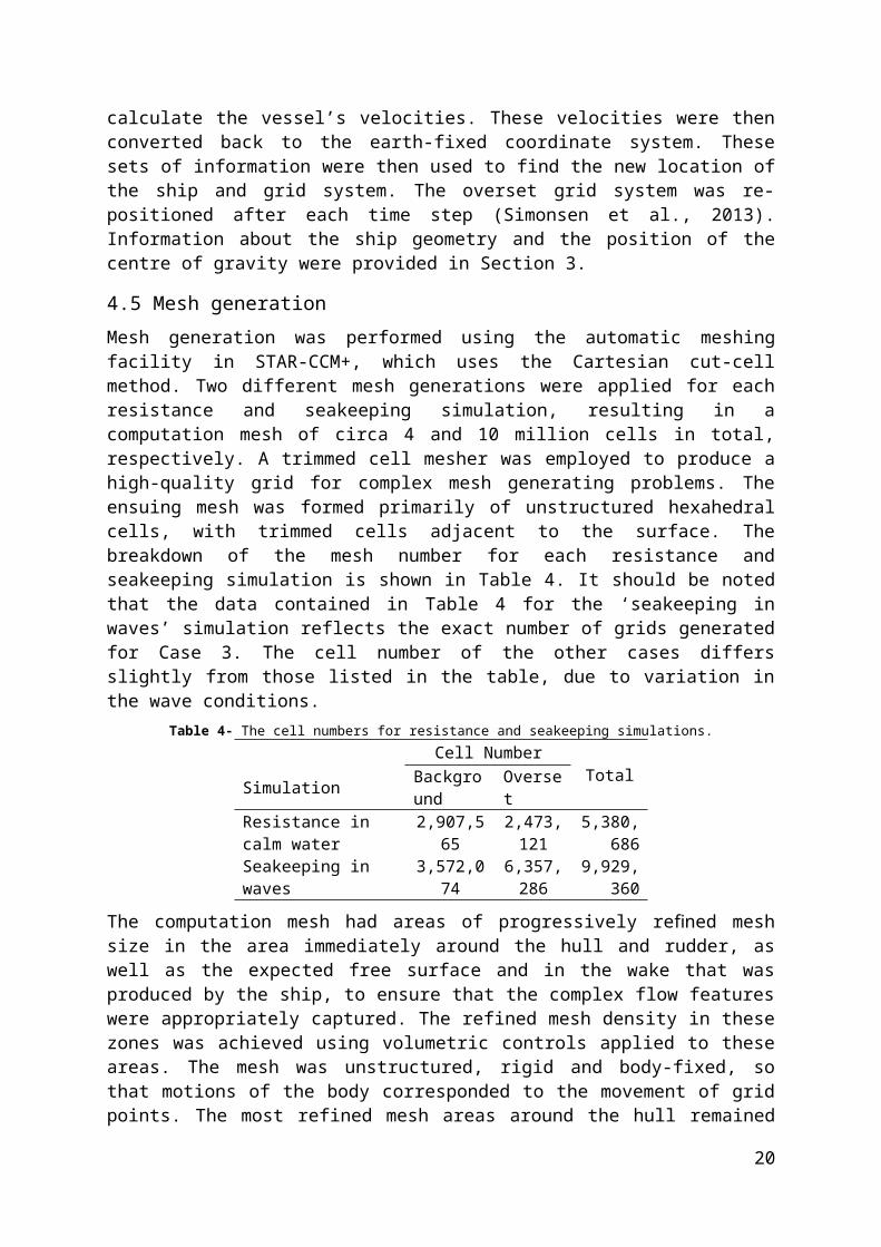
4.5 Mesh generationMesh generation was performed using the automatic meshing facility in STAR-CCM+, which uses the Cartesian cut-cell method. Two different mesh generations were applied for each resistance and seakeeping simulation, resulting in a computation mesh of circa 4 and 10 million cells in total, respectively. A trimmed cell mesher was employed to produce a high-quality grid for complex mesh generating problems. The ensuing mesh was formed primarily of unstructured hexahedral cells, with trimmed cells adjacent to the surface. The breakdown of the mesh number for each resistance and seakeeping simulation is shown in Table 4. It should be noted that the data contained in Table 4 for the ‘seakeeping in waves’ simulation reflects the exact number of grids generated for Case 3. The cell number of the other cases differs slightly from those listed in the table, due to variation in the wave conditions.
Table 4- The cell numbers for resistance and seakeeping simulations.Cell Number
TotalSimulation Backgroun
d Overset
Resistance in calm water 2,907,565 2,473,12
15,380,68
6
Seakeeping in waves 3,572,074 6,357,286
9,929,360
The computation mesh had areas of progressively refined mesh size in the area immediately around the hull and rudder, as well as the expected free surface and in the wake that was produced by the ship, to ensure that the complex flow features were appropriately captured. The refined mesh density in these zones was achieved using volumetric controls applied to these areas. The mesh was unstructured, rigid and body-fixed, so that motions of the body corresponded to the movement of grid points. The most refined mesh areas around the hull remained within the boundaries of the overset domain. When generating the volume mesh, extra care was given to the overlapping zone between the background and overset regions. CD-Adapco (2014) can be consulted for any further information as to how to generate suitable meshes when working with the overset mesh feature.
To simulate ship motions in waves, the mesh was generated based on the guidelines for ship CFD applications from ITTC (2011a). According to these recommendations, a minimum of 80 cells per wavelength should be used on the free surface. As suggested by Kim and Lee (2011), in order to capture the severe free surface flows such as slamming and green water incidents, a minimum of 150 grid points per wavelength was used near the hull free surface in both downstream and upstream directions. Additionally, a minimum of 20 cells was used in the vertical direction where the free surface was expected.
When generating the mesh for the simulations in calm water, the refined mesh area for the free surface was kept relatively small, compared to that used in the seakeeping simulations. In this case, based on prior experience, a minimum cell size of 0.0785% of LBP in the vertical direction was used to capture the flow features in the free surface.
13
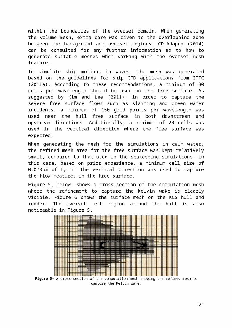
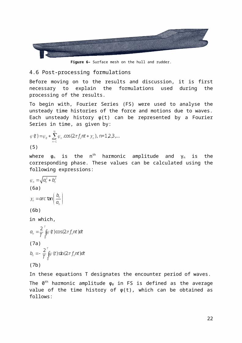
Figure 5, below, shows a cross-section of the computation mesh where the refinement to capture the Kelvin wake is clearly visible. Figure 6 shows the surface mesh on the KCS hull and rudder. The overset mesh region around the hull is also noticeable in Figure 5.
Figure 5– A cross-section of the computation mesh showing the refined mesh to capture the Kelvin wake.
Figure 6– Surface mesh on the hull and rudder.
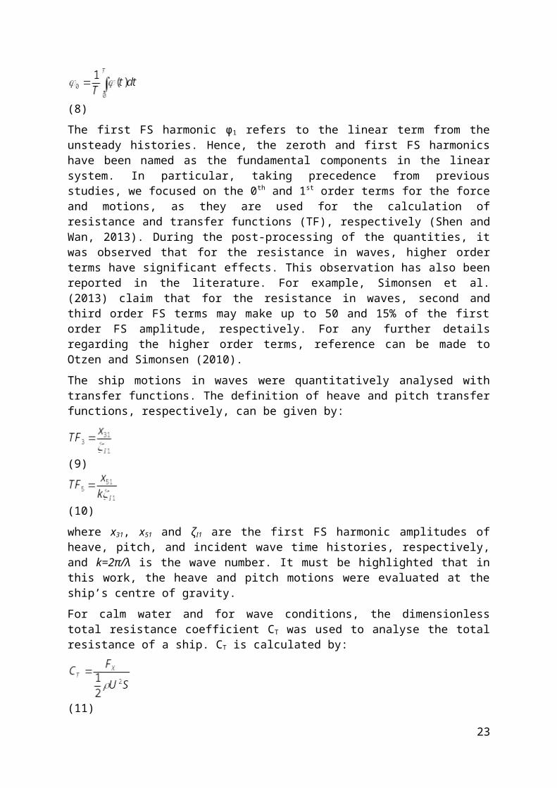
4.6 Post-processing formulationsBefore moving on to the results and discussion, it is first necessary to explain the formulations used during the processing of the results.
To begin with, Fourier Series (FS) were used to analyse the unsteady time histories of the force and motions due to waves. Each unsteady history φ(t) can be represented by a Fourier Series in time, as given by:
(5)
where φn is the nth harmonic amplitude and γn is the corresponding phase. These values can be calculated using the following expressions:
(6a)
(6b)
in which,
(7a)
(7b)
In these equations T designates the encounter period of waves.
14
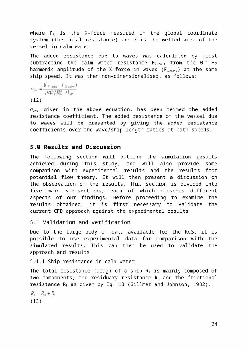
The 0th harmonic amplitude φ0 in FS is defined as the average value of the time history of φ(t), which can be obtained as follows:
(8)
The first FS harmonic φ1 refers to the linear term from the unsteady histories. Hence, the zeroth and first FS harmonics have been named as the fundamental components in the linear system. In particular, taking precedence from previous studies, we focused on the 0 th and 1st
order terms for the force and motions, as they are used for the calculation of resistance and transfer functions (TF), respectively (Shen and Wan, 2013). During the post-processing of the quantities, it was observed that for the resistance in waves, higher order terms have significant effects. This observation has also been reported in the literature. For example, Simonsen et al. (2013) claim that for the resistance in waves, second and third order FS terms may make up to 50 and 15% of the first order FS amplitude, respectively. For any further details regarding the higher order terms, reference can be made to Otzen and Simonsen (2010).
The ship motions in waves were quantitatively analysed with transfer functions. The definition of heave and pitch transfer functions, respectively, can be given by:
(9)
(10)
where x31, x51 and ζI1 are the first FS harmonic amplitudes of heave, pitch, and incident wave time histories, respectively, and k=2π/λ is the wave number. It must be highlighted that in this work, the heave and pitch motions were evaluated at the ship’s centre of gravity.
For calm water and for wave conditions, the dimensionless total resistance coefficient CT was used to analyse the total resistance of a ship. CT is calculated by:
(11)
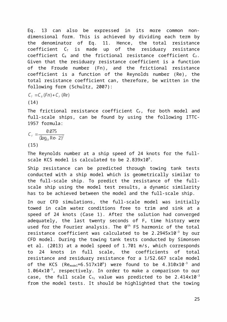
where FX is the X-force measured in the global coordinate system (the total resistance) and S is the wetted area of the vessel in calm water.
The added resistance due to waves was calculated by first subtracting the calm water resistance FX,calm from the 0th FS harmonic amplitude of the X-force in waves (FX,wave) at the same ship speed. It was then non-dimensionalised, as follows:
(12)
σaw, given in the above equation, has been termed the added resistance coefficient. The added resistance of the vessel due to waves will be presented by giving the added resistance coefficients over the wave/ship length ratios at both speeds.
15
5.0 Results and DiscussionThe following section will outline the simulation results achieved during this study, and will also provide some comparison with experimental results and the results from potential flow theory. It will then present a discussion on the observation of the results. This section is divided into five main sub-sections, each of which presents different aspects of our findings. Before proceeding to examine the results obtained, it is first necessary to validate the current CFD approach against the experimental results.
5.1 Validation and verificationDue to the large body of data available for the KCS, it is possible to use experimental data for comparison with the simulated results. This can then be used to validate the approach and results.
5.1.1 Ship resistance in calm water
The total resistance (drag) of a ship RT is mainly composed of two components; the residuary resistance RR and the frictional resistance RF as given by Eq. 13 (Gillmer and Johnson, 1982).
(13)
Eq. 13 can also be expressed in its more common non-dimensional form. This is achieved by dividing each term by the denominator of Eq. 11. Hence, the total resistance coefficient CT is made up of the residuary resistance coefficient CR and the frictional resistance coefficient CF. Given that the residuary resistance coefficient is a function of the Froude number (Fn), and the frictional resistance coefficient is a function of the Reynolds number (Re), the total resistance coefficient can, therefore, be written in the following form (Schultz, 2007):
(14)
The frictional resistance coefficient CF, for both model and full-scale ships, can be found by using the following ITTC-1957 formula:
(15)
The Reynolds number at a ship speed of 24 knots for the full-scale KCS model is calculated to be 2.839x10⁹.
Ship resistance can be predicted through towing tank tests conducted with a ship model which is geometrically similar to the full-scale ship. To predict the resistance of the full-scale ship using the model test results, a dynamic similarity has to be achieved between the model and the full-scale ship.
In our CFD simulations, the full-scale model was initially towed in calm water conditions free to trim and sink at a speed of 24 knots (Case 1). After the solution had converged adequately, the last twenty seconds of Fx time history were used for the Fourier analysis. The 0th FS harmonic of the total resistance coefficient was calculated to be 2.2945x10⁻³ by our CFD model. During the towing tank tests conducted by Simonsen et al. (2013) at a model speed of 1.701 m/s, which corresponds to 24 knots in full scale, the coefficients of total resistance and residuary resistance for a 1/52.667 scale model of the KCS (Remodel=6.517x10⁶) were found to be 4.310x10⁻³ and 1.064x10⁻³, respectively. In order to make a comparison to our case, the full scale CTs value was predicted to be 2.414x10⁻³ from the model tests. It
16
should be highlighted that the towing tank experiments were also conducted in trim and sinkage free conditions.
As can clearly be seen from the above calculations, the CT value of the vessel in calm water at 24 knots is quite compatible with the experiments, and is only under-predicted by 4.95% compared to the towing tank results.
5.1.2 Wave generation
5th-order Stokes waves were used inside the computational domain throughout all simulations. The theory of the 5th-order wave is based on the work by Fenton (1985). The reason for selecting this wave is that according to CD-Adapco (2014), “this wave more closely resembles a real wave than one generated by the first order method”. The first order wave mentioned here is the wave that generates a regular periodic sinusoidal profile.
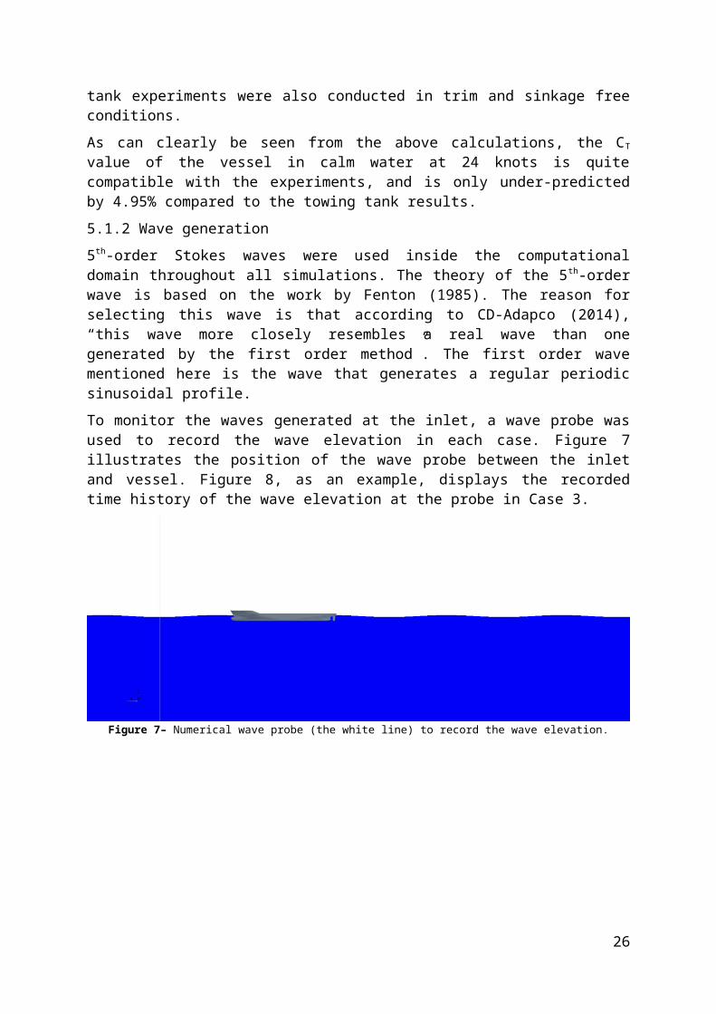
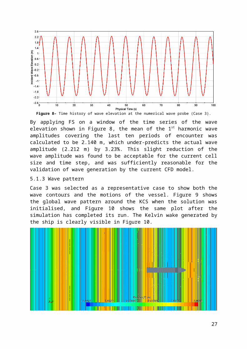
To monitor the waves generated at the inlet, a wave probe was used to record the wave elevation in each case. Figure 7 illustrates the position of the wave probe between the inlet and vessel. Figure 8, as an example, displays the recorded time history of the wave elevation at the probe in Case 3.
Figure 7– Numerical wave probe (the white line) to record the wave elevation.
Figure 8– Time history of wave elevation at the numerical wave probe (Case 3).
By applying FS on a window of the time series of the wave elevation shown in Figure 8, the mean of the 1st harmonic wave amplitudes covering the last ten periods of encounter was calculated to be 2.140 m, which under-predicts the actual wave amplitude (2.212 m) by
17
3.23%. This slight reduction of the wave amplitude was found to be acceptable for the current cell size and time step, and was sufficiently reasonable for the validation of wave generation by the current CFD model.
5.1.3 Wave pattern
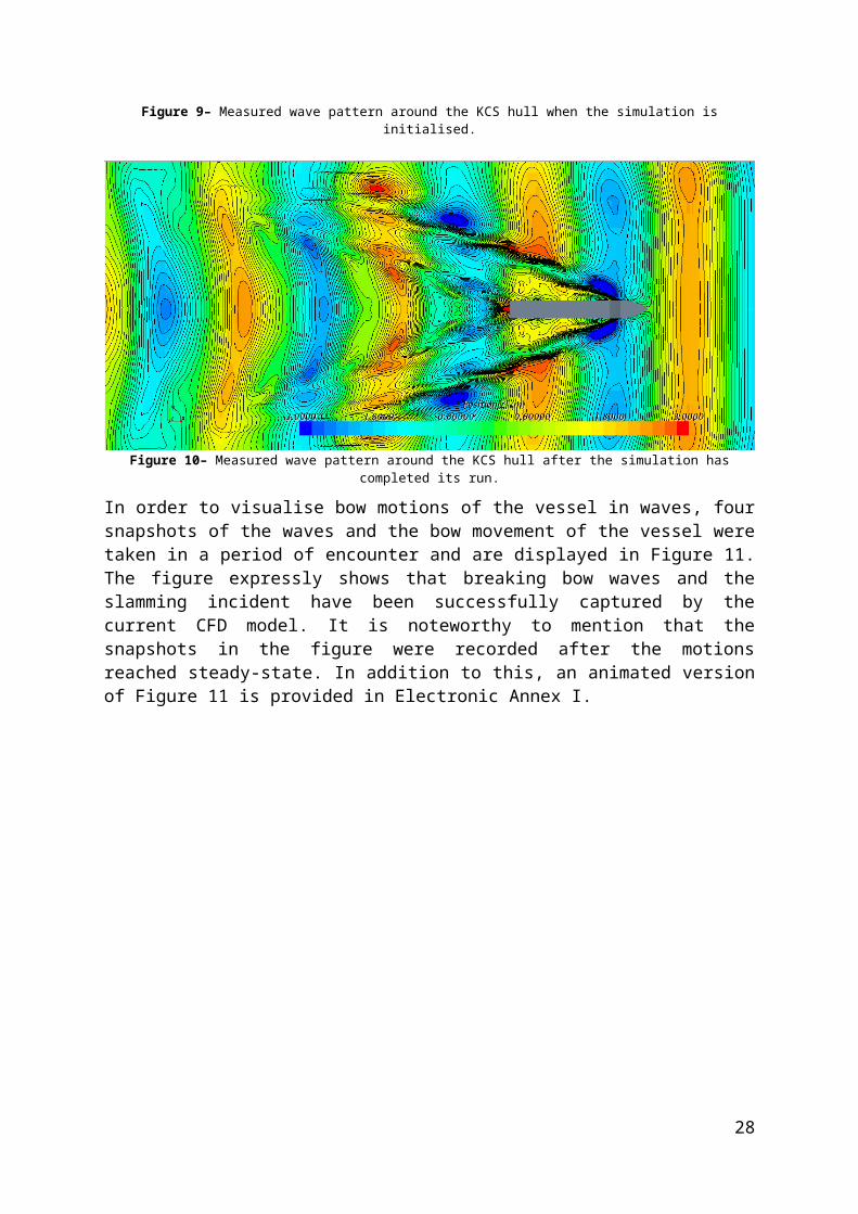
Case 3 was selected as a representative case to show both the wave contours and the motions of the vessel. Figure 9 shows the global wave pattern around the KCS when the solution was initialised, and Figure 10 shows the same plot after the simulation has completed its run. The Kelvin wake generated by the ship is clearly visible in Figure 10.
Figure 9– Measured wave pattern around the KCS hull when the simulation is initialised.
Figure 10– Measured wave pattern around the KCS hull after the simulation has completed its run.
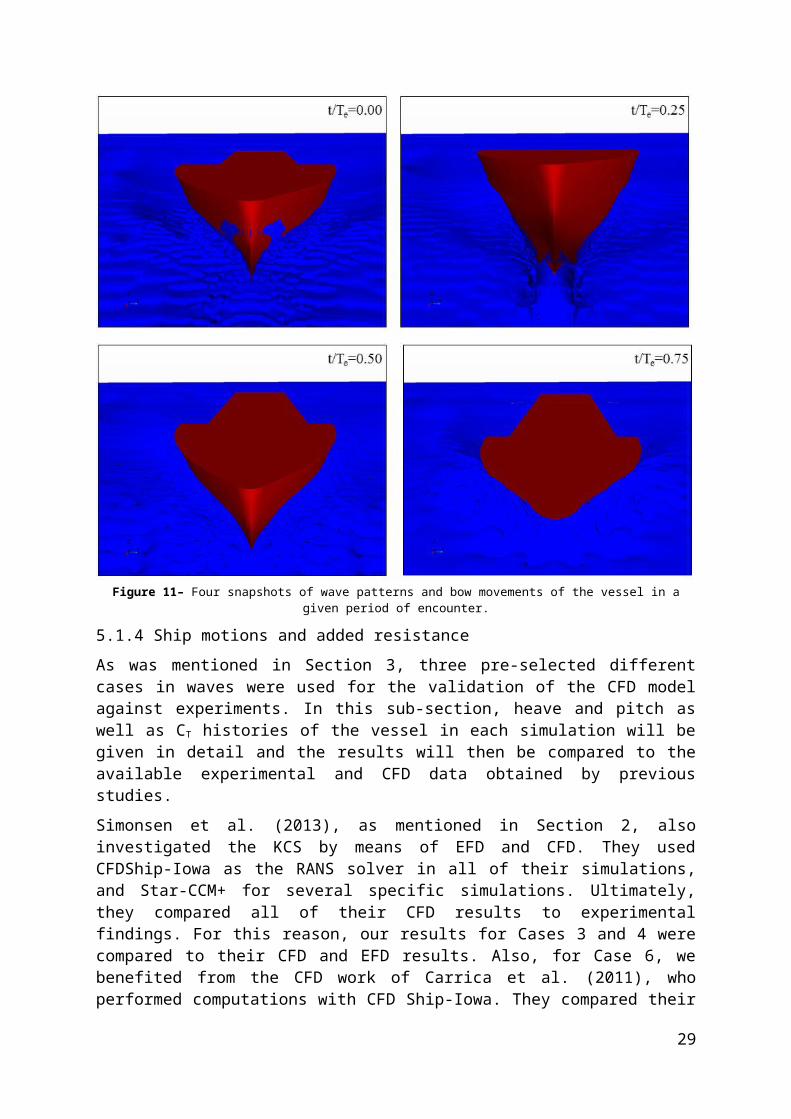
In order to visualise bow motions of the vessel in waves, four snapshots of the waves and the bow movement of the vessel were taken in a period of encounter and are displayed in Figure11. The figure expressly shows that breaking bow waves and the slamming incident have been successfully captured by the current CFD model. It is noteworthy to mention that the snapshots in the figure were recorded after the motions reached steady-state. In addition to this, an animated version of Figure 11 is provided in Electronic Annex I.
18
Figure 11– Four snapshots of wave patterns and bow movements of the vessel in a given period of encounter.
5.1.4 Ship motions and added resistance
As was mentioned in Section 3, three pre-selected different cases in waves were used for the validation of the CFD model against experiments. In this sub-section, heave and pitch as well as CT histories of the vessel in each simulation will be given in detail and the results will then be compared to the available experimental and CFD data obtained by previous studies.
Simonsen et al. (2013), as mentioned in Section 2, also investigated the KCS by means of EFD and CFD. They used CFDShip-Iowa as the RANS solver in all of their simulations, and Star-CCM+ for several specific simulations. Ultimately, they compared all of their CFD results to experimental findings. For this reason, our results for Cases 3 and 4 were compared to their CFD and EFD results. Also, for Case 6, we benefited from the CFD work of Carrica et al. (2011), who performed computations with CFD Ship-Iowa. They compared their results with the experimental study of Otzen and Simonsen (2010), as well as with the CFD results of several researchers, who used different numerical approaches.
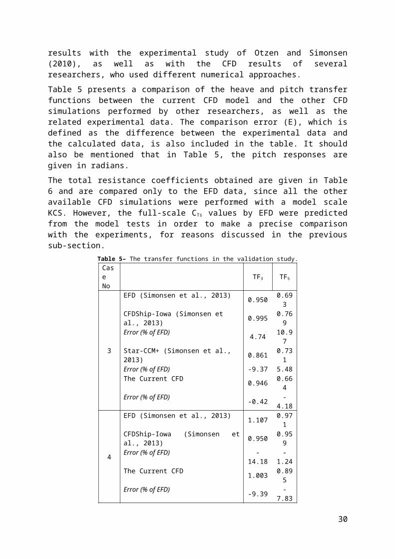
Table 5 presents a comparison of the heave and pitch transfer functions between the current CFD model and the other CFD simulations performed by other researchers, as well as the related experimental data. The comparison error (E), which is defined as the difference between the experimental data and the calculated data, is also included in the table. It should also be mentioned that in Table 5, the pitch responses are given in radians.
The total resistance coefficients obtained are given in Table 6 and are compared only to the EFD data, since all the other available CFD simulations were performed with a model scale KCS. However, the full-scale CTs values by EFD were predicted from the model tests in order
19
to make a precise comparison with the experiments, for reasons discussed in the previous sub-section.
Table 5– The transfer functions in the validation study.Case No TF3 TF5
3
EFD (Simonsen et al., 2013) 0.950 0.693CFDShip-Iowa (Simonsen et al., 2013) 0.995 0.769Error (% of EFD) 4.74 10.97Star-CCM+ (Simonsen et al., 2013) 0.861 0.731Error (% of EFD) -9.37 5.48The Current CFD 0.946 0.664Error (% of EFD) -0.42 -4.18
4
EFD (Simonsen et al., 2013) 1.107 0.971CFDShip-Iowa (Simonsen et al., 2013) 0.950 0.959Error (% of EFD) -14.18 -1.24The Current CFD 1.003 0.895Error (% of EFD) -9.39 -7.83
6
EFD (Otzen and Simonsen, 2010) 0.901 1.037CFDShip-Iowa (P. M. Carrica et al., 2011) 0.854 0.993Error (% of EFD) -5.2 -4.2CFD (El Moctar et al., 2010) 0.891 1.044Error (% of EFD) -1.1 0.6CFD (Manzke and Rung, 2010) 0.958 1.184Error (% of EFD) 6.3 -14.1CFD (Akimoto et al., 2010) 1.255 1.037Error (% of EFD) 39.2 0The Current CFD 0.847 1.085Error (% of EFD) -5.99 4.63
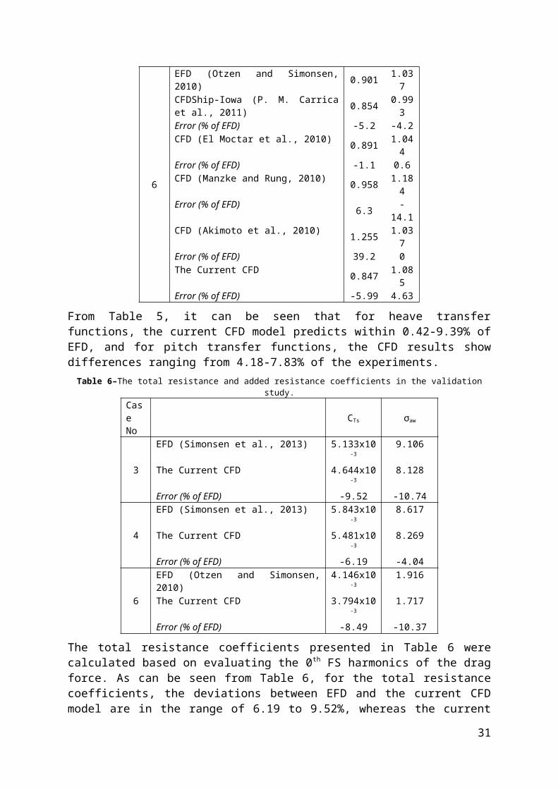
From Table 5, it can be seen that for heave transfer functions, the current CFD model predicts within 0.42-9.39% of EFD, and for pitch transfer functions, the CFD results show differences ranging from 4.18-7.83% of the experiments.
Table 6–The total resistance and added resistance coefficients in the validation study.Case No CTs σaw
3EFD (Simonsen et al., 2013) 5.133x10⁻³ 9.106The Current CFD 4.644x10⁻³ 8.128Error (% of EFD) -9.52 -10.74
4EFD (Simonsen et al., 2013) 5.843x10⁻³ 8.617The Current CFD 5.481x10⁻³ 8.269Error (% of EFD) -6.19 -4.04
6EFD (Otzen and Simonsen, 2010) 4.146x10⁻³ 1.916The Current CFD 3.794x10⁻³ 1.717Error (% of EFD) -8.49 -10.37
The total resistance coefficients presented in Table 6 were calculated based on evaluating the 0th FS harmonics of the drag force. As can be seen from Table 6, for the total resistance coefficients, the deviations between EFD and the current CFD model are in the range of 6.19 to 9.52%, whereas the current CFD model underpredicts the added resistance coefficients within approximately 10% of the experimental data.
For the purpose of visualisation, Figure 12 displays how the vessel responds to incident head seas in a period of encounter. The pictures are snapshots from the simulation of Case 3 after the solution has stabilised. The corresponding animation for this figure is provided in Electronic Annex II.
20
Figure 12– Four snapshots of motions of the vessel and the free surface in a given period of encounter.
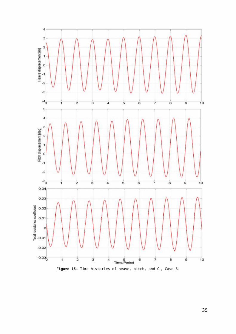
The time histories of heave, pitch and CT that belong to all the validation cases, as shown in Figures Figure 13-Figure 15, were recorded over the last ten periods of encounter.
21
Figure 13– Time histories of heave, pitch, and CT, Case 3.
22
Figure 14– Time histories of heave, pitch, and CT, Case 4.
23
Figure 15– Time histories of heave, pitch, and CT, Case 6.
24
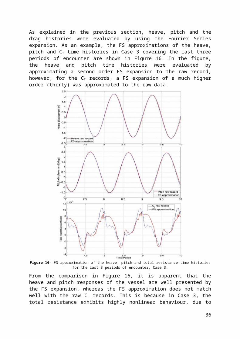
As explained in the previous section, heave, pitch and the drag histories were evaluated by using the Fourier Series expansion. As an example, the FS approximations of the heave, pitch and CT time histories in Case 3 covering the last three periods of encounter are shown in Figure 16. In the figure, the heave and pitch time histories were evaluated by approximating a second order FS expansion to the raw record, however, for the CT records, a FS expansion of a much higher order (thirty) was approximated to the raw data.
Figure 16– FS approximation of the heave, pitch and total resistance time histories for the last 3 periods of encounter, Case 3.
From the comparison in Figure 16, it is apparent that the heave and pitch responses of the vessel are well presented by the FS expansion, whereas the FS approximation does not match well with the raw CT records. This is because in Case 3, the total resistance exhibits highly nonlinear behaviour, due to resonance. However, this should not pose a problem since the zeroth FS harmonics are used in CT calculations. The same approach is also used when evaluating experimental time records. Also, it should be borne in mind that in Cases 4 and 6, the total resistance time histories are much closer to linearity (see Figures Figure 14 and Figure 15).
5.1.5 Verification study
25
A verification study was undertaken to assess the simulation numerical uncertainty, USN, and numerical errors, δSN. In the present work, it was assumed that the numerical error is composed of iterative convergence error (δI), grid-spacing convergence error (δG) and time-step convergence error (δT), which gives the following expressions for the simulation numerical error and uncertainty (Stern et al., 2001):
(16)
(17)
where UI, UG and UT are the uncertainties arising from the iterative, grid-spacing convergence, and time-step convergence errors, respectively.
The verification study was carried out for the resonant case (Case 3) because, according to Weymouth et al. (2005), large motions and accelerations tend to cause the highest numerical errors. This therefore can be regarded as a ‘worst-case test’.
Xing and Stern (2010) state that the Richardson extrapolation method (Richardson, 1911) is the basis for existing quantitative numerical error/uncertainty estimates for time-step convergence and grid-spacing. With this method, the error is expanded in a power series, with integer powers of grid-spacing or time-step taken as a finite sum. Commonly, only the first term of the series will be retained, assuming that the solutions lie in the asymptotic range. This practice generates a so-called grid-triplet study. Roache’s (1998) grid convergence index (GCI) is useful for estimating uncertainties arising from grid-spacing and time-step errors. Roache’s GCI is recommended for use by both the American Society of Mechanical Engineers (ASME) (Celik et al., 2008) and the American Institute of Aeronautics and Astronautics (AIAA) (Cosner et al., 2006).
For estimating iterative errors, the procedure derived by Roy and Blottner (2001) was used. The results obtained from these calculations suggest that the iterative errors for TF3, TF5, and CT are 0.181, 0.164, and 0.312% of the solution for the finest grid and smallest time-step.
Grid-spacing and time-step convergence studies were carried out following the correlation factor (CF) and GCI methods of Stern et al. (2006). The convergence studies were performed with triple solutions using systematically refined grid-spacing or time-steps. For example, the grid convergence study was conducted using three calculations in which the grid size was systematically coarsened in all directions whilst keeping all other input parameters (such as time-step) constant. The mesh convergence analysis was carried out with the smallest time-step, whereas the time-step convergence analysis was carried out with the finest grid size.
To assess the convergence condition, the convergence ratio is used as given in Eq. (18):
(18)
In Eq. (18) εk21=Sk2-Sk1 and εk32=Sk3-Sk2 are the differences between medium-fine and coarse-medium solutions, where Sk1, Sk2, Sk3 correspond to the solutions with fine, medium, and coarse input parameters, respectively. The subscript k refers to the kth input parameter (i.e. grid-size or time-step) (Stern et al., 2006).
Four typical convergence conditions may be seen: (i) monotonic convergence (0<Rk<1), (ii) oscillatory convergence (Rk<0; |Rk|<1), (iii) monotonic divergence (Rk>1), and (iv) oscillatory divergence (Rk<0; |Rk|>1) (Stern et al., 2006).
26
For condition (i), the generalised Richardson extrapolation method is used to predict the numerical error and uncertainties. For condition (ii), the uncertainty is predicted by:
(19)
where SU and SL are the maximum and minimum of the solutions from the corresponding convergence study. For diverging conditions (iii) and (iv), neither error nor uncertainty can be assessed (Stern et al., 2006).
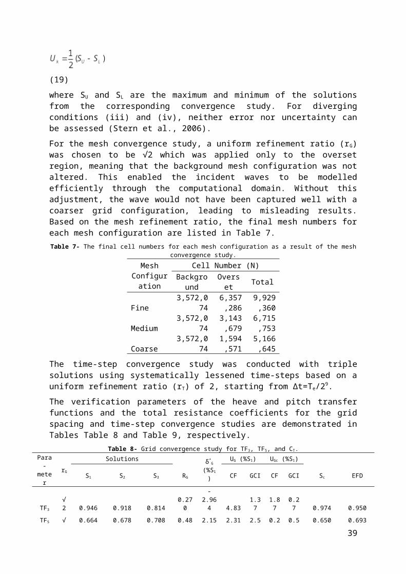
For the mesh convergence study, a uniform refinement ratio (rG) was chosen to be √2 which was applied only to the overset region, meaning that the background mesh configuration was not altered. This enabled the incident waves to be modelled efficiently through the computational domain. Without this adjustment, the wave would not have been captured well with a coarser grid configuration, leading to misleading results. Based on the mesh refinement ratio, the final mesh numbers for each mesh configuration are listed in Table 7.
Table 7- The final cell numbers for each mesh configuration as a result of the mesh convergence study.
Mesh Configurati
on
Cell Number (N)Backgrou
nd Overset Total
Fine 3,572,0746,357,28
69,929,36
0
Medium 3,572,0743,143,67
96,715,75
3
Coarse 3,572,0741,594,57
15,166,64
5
The time-step convergence study was conducted with triple solutions using systematically lessened time-steps based on a uniform refinement ratio (rT) of 2, starting from Δt=Te/29.
The verification parameters of the heave and pitch transfer functions and the total resistance coefficients for the grid spacing and time-step convergence studies are demonstrated in Tables Table 8 and Table 9, respectively.
Table 8- Grid convergence study for TF3, TF5, and CT.
In Tables Table 8 and Table 9, the corrected simulation value (Sc) is calculated by Sc=S- δ*G,
where S is the simulation result. Also, Uc is the corrected uncertainty. For more detailed information on how to calculate these uncertainties, reference can be made to Stern et al.
27
(2006). The notation style of this reference was used in this study, to enable the verification results to be presented clearly.
As can be seen from the results listed in Tables Table 8 and Table 9, reasonably small levels of uncertainty were estimated for the motion transfer functions. On the other hand, relatively large uncertainties UG (16.53% and 9.75%) were predicted for CT, using the CF and GCI methods, respectively. However, these values reduce to 4.37% and 1.95%, respectively, when the corrected uncertainties (UGc) are estimated. This implies that the total drag force in the resonant case is very sensitive to the grid size resolution. It is expected that the uncertainties for the total resistance coefficient in the other cases are smaller than those in Case 3.
As a result of the convergence studies, corrected and uncorrected verification parameters of the heave and pitch transfer functions and the total resistance coefficients are given in Table10. In the table, the subscript c refers to the corrected parameters.
Stern et al. (2006) specify that in order to determine whether a validation has been successful, the comparison error E must be compared to UV, the validation uncertainty, given by
(20)
where UD is the uncertainty in experimental data, which is 5.83% in Simonsen et al.’s EFD data.
Table 10- Validation of heave and pitch transfer functions and total resistance coefficient.
Para-meter
USN (%EFD)UD
UV
(%EFD) E (%)CF GCI CF GCI
TF3 4.89 1.70 5.83 7.61 6.07 -0.42
TF3c 1.87 0.38 5.83 6.12 5.84 3.07
TF5 2.52 2.51 5.83 6.35 6.35 -4.18
TF5c 0.33 0.53 5.83 5.84 5.85 -5.52
CT 15.02 9.24 5.83 16.1110.9
2 -9.52
CTc 4.00 1.87 5.83 7.07 6.12 -5.01
Since the absolute value of the comparison error E is smaller than UV, the heave and pitch transfer functions, as well as the total resistance coefficient, were validated for both the corrected and uncorrected case. The uncertainty levels were estimated to be 6.12%, 5.84% and 7.07%, respectively, when calculated using the CF method. When the GCI method is used to assess these uncertainties, these values become 5.84%, 5.85% and 6.12%, respectively.
5.2 Calm water results Having validated the CFD model, and having performed the necessary verification study, the reminder of this section addresses the main findings of this work.
The calm water total resistance coefficients (CT), the dynamic sinkage results non-dimensionalised with the ship length (x30/LBP) and the trim angle (x50) in degrees are presented for two speeds in Table 11. The CFD results contained in Table 11 for 24 knots are under-predicted by approximately 6.7% compared to the towing tank results of Simonsen et al. (2013). The estimation of the full scale CT value at 24 knots through the towing tank tests was explained in the previous sub-section. Unfortunately, experimental results for this ship
28
operating at a speed of 19 knots are not available in the literature, and thus could not be included in this paper. The quantities listed in the table decrease as the ship speed is reduced to 19 knots, as expected.
Table 11- Calm water results.Speed (kn) CT x30/LBP x50 (deg)
24
EFD (Simonsen et al., 2013) 0.002414 -0.0021 0.1853
5.3 Ship motion responses in head seas The results obtained using the proposed RANS method were compared to those obtained using the potential theory-based frequency domain code VERES. In the potential theory the fluid is assumed to be homogeneous, non-viscous, irrotational and incompressible. The method used to calculate ship motions in VERES is based on the two-dimensional, linear, strip theory formulation by Salvesen, Tuck and Faltinsen (1970). For more information about this seakeeping code, reference can be made to the theory manual of the software (Fathi and Hoff, 2013).
Heave and pitch transfer functions predicted by CFD, EFD and VERES at the two different speeds, listed in Table 12, are illustrated graphically in Figures Figure 17 and Figure 18. This gives a clearer depiction of the responses of the vessel to head waves, enabling a more facile comparison among the different approaches. The comparison errors are also listed in Table12. The EFD data are taken from Simonsen et al. (2013).
Table 12– The transfer functions for all cases by three different methods (Error (E) is based on EFD data).
Case no.
Ship speed (kn)
Froude numbe
r
TF3 TF5
CFDEFD
VERES CFDEFD
VERES
C U Fn Result E (%) Result E (%) Result E (%) Result E (%)
Figure 17– A comparison of the ship motions using different methods at a speed of 24 knots(the left- and right-hand sides of the graph show heave and pitch TFs, respectively).
Figure 18– A comparison of the ship motions by CFD and potential theory at a speed of 19 knots(the left- and right-hand sides of the graph show heave and pitch TFs, respectively).
As clearly seen from Figure 17 and Table 12, compared to the EFD, the motions are generally better predicted by the CFD method than by the potential theory-based software package, particularly for heave motion. When Figures Figure 17 and Figure 18 are compared with each other, the discrepancies between the CFD and VERES are much more pronounced at 24 knots. Generally, VERES seems to overpredict the motions compared to the CFD method, particularly at 19 knots. Additionally, as can be understood from Table 12, the heave and pitch responses of the vessel tend to decrease at 19 knots, compared to those at 24 knots. However, it is predicted that although the vessel decreases its speed when operating in head seas where λ/L=1.0, the heave and pitch responses increase at 19 knots (in Case 8). This is due to the fact that the encounter frequency in that wave condition becomes close to the natural heave and pitch frequency as the speed is reduced to 19 knots.
5.4 Resistance coefficientsThe resultant added resistance and total resistance coefficients of the vessel in question using the different methods are tabulated in Table 13, below. Also, the comparison errors which are based on EFD data are listed in the table. Since the experimental CT values are not available, only the results from CFD and potential theory calculations are given for the total resistance coefficients in the table. In addition, the added resistance coefficients at both ship speeds are shown graphically in Figure 19.
For the added resistance calculations, the employed potential theory-based software uses the method of Gerritsma and Beukelman (1972), which is based on the determination of the energy of the radiating waves and a strip-theory approximation (Fathi and Hoff, 2013).
30
Table 13– The added resistance and total resistance coefficients for all cases using different methods(Error (E) is based on EFD data).
Case no.
Ship speed (kn)
Froude number
σaw
CTsx10-3
CFDEFD
VERES
C U Fn Result E (%) Result E (%) CFD VERES
1
24 0.260
calm water 2.295 2.182
2 6.595 -9.19 7.263 6.198 -17.95 3.726 3.527
3 8.128 -10.74 9.106 7.517 -17.45 4.644 4.355
4 8.269 -4.04 8.617 5.315 -38.32 5.481 4.230
5 5.175 -8.82 5.676 3.476 -38.76 4.822 3.879
6 1.717 -10.37 1.916 1.214 -36.62 3.794 3.242
7
19 0.206
calm water 1.923 1.569
8 5.159 - - 6.021 - 3.709 3.654
9 5.073 - - 5.233 - 4.263 3.982
10 3.648 - - 3.352 - 4.166 3.630
11 2.345 - - 2.212 - 3.750 3.292
12 1.064 - - 0.801 - 3.406 2.684
Figure 19– A comparison of the added resistance coefficients using different methods at two ship speeds(the left- and right-hand sides of the graph show ship speeds of 19 and 24 knots, respectively).
As Table 13 and Figure 19 jointly show, for the added resistance coefficients, CFD agrees much better with the experiments when compared to VERES for the ship speed of 24 knots. Both methods underpredict the added resistance coefficients compared to the EFD data. When the added resistance predictions at the two speeds are compared, it is obvious that the discrepancies between VERES and CFD are much more pronounced at 24 knots, in a similar manner to the ship motion predictions. This is expected, because the results obtained from the linear potential theory are more accurate at moderate speeds than at higher speeds.
5.5 Increases in the effective power of the vessel due to added resistanceThe effective power (PE) is the power required to propel the vessel forward through the water at a constant speed, and is thus calculated as the product of the speed and the total resistance. The effective power can be computed using CFD approaches such as the one which is demonstrated in this paper, however this is not the case for the fuel consumption. This is due to the very complex interplay of the variables that contribute to fuel consumption, such as engine load, SFOC (Specific Fuel Oil Consumption), propeller speeds and many others, which depend on a vessel’s specifics at different operating conditions. Therefore, in this paper, the fuel consumption will not be calculated directly. Instead, the percentage increase in effective power due to the added resistance in waves will be calculated as given by Eq. 21. This can be taken as an indication of the implications for fuel consumption, and hence CO2
31
emissions, of the vessel in question operating in a seaway, assuming that efficiencies and SFOC remain constant.
(21)
Figures Figure 20 and Figure 21 show the predictions of the percentage increase in the effective power, fuel consumption, and hence CO2 emissions of the KCS due to induced added resistance at ship speeds of 24 and 19 knots, respectively. The calculations were performed based on the formula given in Eq. 21. It should be emphasised that when calculating the increase in PE, the difference in CT between the wave and calm conditions should be considered at the same speed.
Figure 20–Estimation of the percentage increase in the effective power, fuel consumption and CO2 emissions of the KCS due to operation in head seas at 24 knots.
Figure 21–Estimation of the percentage increase in the effective power, fuel consumption and CO2 emissions of the KCS due to operation in head seas at 19 knots.
According to Figure 20, CFD calculations imply that the maximum increase in PE (139%) at a ship speed of 24 knots is observed in Case 4 (λ/L=1.33). On the other hand, potential theory calculations for the same speed predict the maximum increase (100%) in Case 3 (λ/L=1.15).
32
However, the data contained in Figure 21 show that the highest increase in the effective power at 19 knots is observed in Case 9 for which λ/L=1.15. This increase is estimated to be around 122% by CFD and 154% by VERES. The minimum increase in the effective power at 24 knots is predicted by CFD as Case 2 (62%) and by VERES as Case 6 (49%). Similarly, both CFD and VERES estimate the minimum increase in PE at 19 knots in Case 12 with ratios of around 77% and 71%, respectively.
In order to reveal the potential benefits of applying the slow steaming approach, for each case the difference in the energy consumed during a voyage under the same wave conditions was calculated between 19 and 24 knots. The metric shown in Eq. 23 was used to estimate the change in PE due to slow steaming, which can be taken as an indication of the fuel consumption, and hence CO2 emissions, of the ship in question.
(22)
which can be reduced to:
(23)
where ‘t(19knots)/t(24knots)’ can be termed the transit time ratio between the durations of the voyages for 19 and 24 knots, respectively.
Figure 22 displays the change in the effective power, fuel consumption and CO2 emissions of the vessel due to its operation under a slow steaming speed condition, with respect to its operation at a more typical service speed. This graph can help to interpret the power reduction or increase for any given case using the CFD and potential theory approaches. For example, when the vessel keeps her course in a head sea condition where λ/L=1.33 (Case 4) at a speed of 24 knots, if she were to reduce her speed down to 19 knots in the same wave conditions (Case 10), we estimate that the required effective power will decrease by 52% and 46% using the CFD and potential theory approaches, respectively. Figure 22 distinctly shows the advantages of slow steaming operational conditions in terms of fuel consumption and CO2
emissions.
Figure 22– Estimation of the percentage change in the effective power, fuel consumption, and CO2 emissions of the KCS due to operation in head seas at a slow steaming speed (19 knots), compared to a speed of 24 knots.
33
6.0 Concluding RemarksFully nonlinear unsteady RANS simulations to predict ship motions and the added resistance of a full scale KCS model have been carried out at two speeds, corresponding to service and slow steaming speeds. The analyses have been conducted by utilising a commercial RANS solver, Star-CCM+.
Firstly, it was shown that the total resistance coefficient in calm water at service speed is underpredicted by 4.95% compared to the related towing tank results. For the simulations in the presence of waves, a numerical wave probe was inserted between the inlet and the ship to measure the generated waves. It has then been shown that the mean of the first harmonic wave amplitude (for a representative case) is underpredicted by 3.23% compared to the expected wave amplitude. This was deemed to be sufficient for the applied time step and mesh size resolutions. During the verification and validation study it was demonstrated in detail that the heave and pitch transfer functions, as well as the total resistance coefficient, were validated at uncertainty levels of 5.84%, 5.85%, and 6.12%, respectively, when calculated using the grid convergence index method.
In ship motions and resistance predictions, it was demonstrated that the current CFD model predicts the heave and pitch transfer functions within a range of 0.42-9.39% and 4.18-7.83% of the EFD data, respectively. For the total resistance coefficients in waves, the deviations between EFD and CFD varied from 6.19 to 9.52% of the experiments. Similarly, the added resistance coefficients were underpredicted by CFD, falling within circa 10% of those from experiments.
The results obtained using the current CFD model were also compared to those obtained using potential flow theory. VERES was used as a potential theory-based seakeeping code to predict the motion responses and the added resistance of the vessel in question. Comparisons between CFD simulations, potential flow calculations and experiments indicated that CFD, in most cases, predicts motions and added resistance with more accuracy than potential theory. Additionally, it was revealed that the discrepancies between RANS computations and potential theory in both motions and added resistance are greater at 24 knots than at 19 knots. This is due to the fact that linear potential theory is designed for moderate speeds and thus has some deficiencies when applied at high speeds, as noted in Section 2. More interestingly, both the CFD and the potential flow calculations generally underpredicted the added resistance coefficients of the vessel when compared to EFD at service speed. It must be recalled that the results obtained using both approaches could only be compared to the experiments at service speed, since the literature does not offer any experimental results conducted at 19 knots.
The increase in effective power due to added resistance was also calculated for each individual wave condition. It has been shown in this paper that this can be taken as an indication of the implications for fuel consumption, and hence CO2 emissions, of KCS operating in a seaway, assuming that efficiencies and SFOC remain constant. From CFD calculations it was observed that the maximum increases in the effective power due to operation in waves are 122% and 139% at 19 and 24 knots, respectively. VERES, on the other hand, estimates these values for the same speed as 154% and 100%, respectively.
With the current trend towards operation according to the slow steaming principle, vessels are operating in conditions that are significantly different to those for which they were designed and optimised. It is therefore critical that the impacts of slow steaming upon ship behaviour and performance are well understood. This paper has shown that slow steaming has beneficial effects on reducing ship motions, power requirements, fuel consumption and hence CO2
34
emissions. It has been estimated using the CFD method described in this paper that application of the slow steaming principle can lead to a decrease of up to 52% in effective power and CO2 emissions, compared to a vessel operating in the same wave conditions at 24 knots.
This paper has provided a very useful starting point for investigations into ship behaviour at off-design speeds, specifically at a representative slow steaming speed for container vessels. In addition to this, the impact on ship motions and added resistance of variations in vessel trim and draft should be investigated, specifically off-design conditions. It has already been observed in simulations and real operations that trim optimisation can be used to reduce the resistance of vessels operating under design conditions.
The study should also be extended to incorporate the propeller and appendages, as these will also have a notable effect on ship behaviour and performance. With the propeller present, and a suitable method used to simulate its rotation, further study into the changes in propulsive efficiency due to motions in a seaway could be made.
Another source of added resistance is hull roughness. The added resistance due to hull roughness can be predicted by employing modified wall functions in CFD software as successfully shown by Demirel et al. (2014). A piece of future work may be the prediction of the added resistance of a ship due to waves and hull fouling, by employing a new wall-function in the CFD software. This may provide a better understanding of the total resistance of a vessel under real operational conditions.
AcknowledgementsThe study presented in this paper was carried out as part of the research project: Low Carbon Shipping- A Systems Approach funded by UK Research Council (EPSRC Grant no. EP/H020004/1). The results were obtained using the EPSRC funded ARCHIE-WeSt High Performance Computer (www.archie-west.ac.uk). EPSRC Grant no. EP/K000586/1.
The first author (The Turkish Council of Higher Education Researcher ID: TR111966) gratefully acknowledges the sponsorship of Izmir Katip Celebi University in Turkey, where he has been working as a research assistant, for giving the Turkish Council of Higher Education PhD Scholarship to fully support his PhD research at the University of Strathclyde, Glasgow.
References
Akimoto, H., Omori, T., Saito, H., Masiur, R. (2010). Numerical simulation of KCS container carrier in head wave conditions. In: Proceedings from Gothenburg 2010-A Workshop on Numerical Ship Hydrodynamics, Gothenburg.
Arribas, F.P. (2007). Some methods to obtain the added resistance of a ship advancing in waves. Ocean Engineering, Vol. 34(7), pp. 946-955, doi: 10.1016/j.oceaneng.2006.06.002.
Banks, C., Turan, O., Incecik, A., Theotokatos, G., Izkan, S., Shewell, C., Tian, X. (2013). Understanding ship operating profiles with an aim to improve energy efficient ship operations. In: Proceedings of the Low Carbon Shipping Conference, London, pp. 1–11.
35
Banks, J.B., Phillips, A.B., Bull, P.W., Turnock, S.R. (2010). RANS simulations of the multiphase flow around the KCS hull form. In: Proceedings from Gothenburg 2010-A Workshop on Numerical Ship Hydrodynamics, Gothenburg.
Beck, R.F., Reed, A. (2001). Modern computational methods for ships in a seaway. Transactions of the Society of Naval Architects and Marine Engineers, Vol. 109, pp. 1-51.
Bertram, V., Yasukawa, H. (1996). Rankine source methods for seakeeping problems. Jahrbuch der Schiffbautechnischen Gesellschaft. Springer, pp. 411-425.
Bhushan, S., Xing, T., Carrica, P., Stern, F. (2009). Model- and full-scale URANS simulations of Athena resistance, powering, seakeeping, and 5415 Maneuvering. Journal of Ship Research, Vol. 53(4), pp. 179-198.
Carrica, P.M., Huiping, F., Stern, F. (2011). Computations of self-propulsion free to sink and trim and of motions in head waves of the KRISO container ship (KCS) model. Applied Ocean Research, Vol. 33(4), pp. 309-320, doi: 10.1016/j.apor.2011.07.003.
Carrica, P.M., Paik, K.J., Hosseini, H.S., Stern, F. (2008). URANS analysis of a broaching event in irregular quartering seas. Journal of Marine Science and Technology, Vol. 13(4), pp. 395-407, doi: 10.1007/s00773-008-0022-5.
Carrica, P.M., Wilson, R.V., Noack, R.W., Stern, F. (2007). Ship motions using single-phase level set with dynamic overset grids. Computers & Fluids, Vol. 36(9), pp. 1415-1433, doi: 10.1016/j.compfluid.2007.01.00.
Castiglione, T., Sadat-Hosseini, H., Stern, F., Bova, S. (2013). CFD simulation for sea keeping of Delft catamaran in regular head and oblique waves. In: Proceedings of the 12th International Conference on Fast Sea Transportation (FAST 2013), Amsterdam, the Netherlands.
Castiglione, T., Stern, F., Bova, S., Kandasamy, M. (2011). Numerical investigation of the seakeeping behavior of a catamaran advancing in regular head waves. Ocean Engineering, Vol. 38(16), pp. 1806-1822, doi: 10.1016/j.oceaneng.2011.09.003.
CD-Adapco (2014). User guide STAR-CCM+ Version 9.0.2.
Celik, I.B., Ghia, U., Roache, P.J., Freitas, C.J., Coleman, H.W., Raad, P.E. (2008). Procedure for estimation and reporting of uncertainty due to discretization in CFD applications. Journal of Fluids Engineering, Vol. 130(7), pp. 078001, doi:10.1115/1.2960953.
Cosner, R.R., Oberkampf, W.L., Rumsey, C.L., Rahaim, C.P., Shih, T.I-P. (2006). AIAA Committee on standards for computational fluid dynamics: Status and plans. In: Proceedings of the 44th Aerospace Sciences Meeting and Exhibit, Reno, Nevada, AIAA Paper No. 2006-889.
Date, J.C., Turnock, S.R. (1999). A study into the techniques needed to accurately predict skin friction using RANS solvers with validation against Froude’s historical flat plate
36
experimental data. Southampton, UK, University of Southampton, 62p. (Ship Science Reports, (114)).
Demirel, Y.K., Khorasanchi, M., Turan, O., Incecik, A., Schultz, M.P. (2014). A CFD model for the frictional resistance prediction of antifouling coatings. Ocean Engineering, Vol. 89. pp. 21-31, http://dx.doi.org/10.1016/j.oceaneng.2014.07.017.
El Moctar, B., Kaufmann, J., Ley, J., Oberhagemann, J., Shigunov, V., Zorn, T. (2010). Prediction of ship resistance and ship motions using RANSE. In: Proceedings from Gothenburg 2010-A Workshop on Numerical Ship Hydrodynamics, Gothenburg.
Enger, S., Peric, M., Peric, R. (2010). Simulation of flow around KCS-hull. In: Proceedings from Gothenburg 2010-A Workshop on Numerical Ship Hydrodynamics, Gothenburg.
Faltinsen, O., Zhao, R. (1991). Numerical Prediction of Ship Motions at High Forward Speed. Philosophical Transactions: Physical Sciences and Engineering, Vol. 334, pp. 241-257.
Fathi, D., Hoff, J.R. (2013). ShipX Vessel Responses (VERES) Theory Manual. Marintek Report, Norway.
Fenton, J.D. (1985). A fifth-order Stokes theory for steady waves. Journal of Waterway, Port, Coastal, and Ocean Engineering, Vol. 111(2), pp. 216-234.
Ferziger, J. H., Peric, M. (2002). Computational Methods for Fluid Dynamics (Third Edit.). Springer, Berlin, Germany.
Field, P.L. (2013). Comparison of RANS and potential flow force computations for the ONR Tumblehome hullform in vertical plane radiation and diffraction problems. MSc. thesis, Virginia Polytechnic Institute and State University, Blacksburg, VA.
Gerritsma, J., Beukelman, W. (1972). Analysis of the resistance increase in waves of a fast cargo ship. International Shipbuilding Progress, Vol. 19(217), pp. 285-293.
Gillmer, T.C., Johnson, B. (1982). Introduction to Naval Architecture. Annapolis, MD: US Naval Institute.
Hochbaum, C.A., Vogt, M. (2002). Towards the simulation of seakeeping and maneuvering based on the computation of the free surface viscous flow. In: Proceedings of the 24 th
Symposium on Naval Hydrodynamics, Fukuoka, Japan.
Hochkirch, K., Mallol, B. (2013). On the importance of full-scale CFD simulations for ships. In: Proceedings of the 12th International Conference on Computer Applications and Information Technology in the Maritime Industries (COMPIT 2013), Cortona, Italy, pp. 85-95.
Hu, C., Kashiwagi, M. (2007). Numerical and experimental studies on three dimensional water on deck with a modified Wigley hull. In: Proceedings of the 9th International Conference in Numerical Ship Hydrodynamics, Ann Arbor, Michigan, US.
37
International Maritime Organisation (IMO) (2009). Guidelines for voluntary use of the Ship Energy Efficiency Operational Indicator (EEOI). MEPC.1/Circ.684. London.
International Towing Tank Conference (ITTC) (2011a). Practical guidelines for ship CFD applications. In: Proceedings of the 26th ITTC, Rio de Janeiro – Brazil. Available from: http://ittc.sname.org/CD%202011/pdf%20Procedures%202011/7.5-03-02-03.pdf [Accessed: 1st February 2014].
International Towing Tank Conference (ITTC) (2011b). The specialist committee on computational fluid dynamics-Final report and recommendations to the 26th ITTC. In: Proceedings of the 26th ITTC, Vol. 2, pp. 337-377, Rio de Janeiro – Brazil.
Kim, S.P. (2011). CFD as a seakeeping tool for ship design. International Journal of Naval Architecture and Ocean Engineering, Vol. 3(1), pp. 65-71, doi: 10.3744/jnaoe.2011.3.1.065.
Kim, S.P., Lee, H.H. (2011). Fully nonlinear seakeeping analysis based on CFD simulations. In: Proceedings of the 21st International Offshore and Polar Engineering Conference, Hawaii, USA, pp. 970-974.
Kim, W.J., Van, S.H., Kim, D.H. (2001). Measurement of flows around modern commercial ship models. Experiments in Fluids, Vol. 31(5), pp. 567-578, doi: 10.1007/s003480100332.
Maersk (n.d.). Slow Steaming: The Full Story. Retrieved from http://www.maersk.com/Innovation/WorkingWithInnovation/Documents/Slow Steaming - the full story.pdf [Accessed: 5th January 2014].
Manzke, M., Rung, T. (2010). Resistance prediction and seakeeping analysis with FreSCo+. In: Proceedings from Gothenburg 2010-A Workshop on Numerical Ship Hydrodynamics, Gothenburg.
Mousaviraad, S.M., Carrica, P.M., Stern, F. (2010). Development and validation of harmonic wave group single-run procedure for RAO with comparison to regular wave and transient wave group procedures using RANS. Ocean Engineering, Vol. 37(8-9), pp. 653-666, doi: 10.1016/j.oceaneng.2010.01.001.
Newman, J.N. (1978). The theory of ship motions. Advances in Applied Mechanics, Vol. 18, pp. 221-283.
Orihara, H., Miyata, H. (2003). Evaluation of added resistance in regular incident waves by computational fluid dynamics motion simulation using overlapping grid system. Journal of Marine Science and Technology, Vol. 8(2), pp. 47-60, doi: 10.1007/s00773-003-0163-5.
Otzen, J.F., Simonsen, C.D. (2010). Uncertainty assessment for KCS resistance and propulsion tests in waves. FORCE Technology, Report no. ONRIII187 01, Lyngby.
38
Ozdemir, Y.H., Barlas, B., Yilmaz, T., Bayraktar, S. (2014). Numerical and experimental study of turbulent free surface flow for a fast ship model. Brodogradnja, Vol. 65(1), pp. 39-54.
Paik, K.J., Carrica, P.M., Lee, D., Maki, K. (2009). Strongly coupled fluid-structure interaction method for structural loads on surface ships. Ocean Engineering, Vol. 36(17-18), pp. 1346-1357, doi: 10.1016/j.oceaneng.2009.08.018.
Querard, A.B.G., Temarel, P., Turnock, S.R. (2008). Influence of viscous effects on the hydrodynamics of ship-like sections undergoing symmetric and anti-symmetric motions, using RANS. Proceedings of the ASME 27th International Conference on Offshore Mechanics and Arctic Engineering (OMAE), Estoril, Portugal, Vol. 5, pp. 683-692.
Richardson, L.F. (1911). The approximate arithmetical solution by finite differences of physical problems involving differential equations, with an application to the stresses in a masonry dam. Philosophical Transactions of the Royal Society of London, Series A, Vol. 210, pp. 307-357, doi: 10.1098/rsta.1911.0009.
Roache, P.J. (1998). Verification and Validation in Computational Science and Engineering. Hermosa Publishers, Albuquerque.
Ronen, D. (2011). The effect of oil price on containership speed and fleet size. Journal of the Operational Research Society, 62(1), pp. 211–216. doi:10.1057/jors.2009.169.
Roy, C.J., Blottner, F.G. (2001). Assessment of one- and two-equation turbulence models for hypersonic transitional flows. Journal of Spacecraft and Rockets, Vol. 38(5), pp. 699-710, doi:10.2514/2.3755.
Salvesen, N., Tuck, E.O., Faltinsen, O. (1970). Ship Motions and Sea Loads. Transactions of the Society of Naval Architects and Marine Engineers, Vol. 78, pp. 250–287.
Sato, Y., Miyata, H., Sato, T. (1999). CFD simulation of 3-dimensional motion of a ship in waves: application to an advancing ship in regular heading waves. Journal of Marine Science and Technology, Vol. 4(3), pp. 108-116, doi: 10.1007/s007730050013.
Schmitke, R.T. (1978). Ship sway, roll, and yaw motions in oblique seas. Transactions of the Society of Naval Architects and Marine Engineers, Vol. 86, pp. 26-46.
Schultz, M.P. (2007). Effects of coating roughness and biofouling on ship resistance and powering. Biofouling, Vol. 23(5), pp. 331-341, doi: 10.1080/08927010701461974.
Shen, Z.R., Wan, D.C. (2013). RANS computations of added resistance and motions of a ship in head waves. International Journal of Offshore and Polar Engineering, Vol. 23(4), pp. 263-271.
Simonsen C.D., Stern, F. (2010). CFD simulation of KCS sailing in regular head waves. In: Proceedings from Gothenburg 2010-A Workshop on Numerical Ship Hydrodynamics, Gothenburg.
39
Simonsen, C.D., Otzen, J.F., Joncquez, S., Stern, F. (2013). EFD and CFD for KCS heaving and pitching in regular head waves. Journal of Marine Science and Technology, Vol. 18(4), pp. 435-459, doi: 10.1007/s00773-013-0219-0.
Stern, F., Carrica, P., Kandasamy, M., Ooi, S.K, et al. (2008). Computational hydrodynamic tools for high-speed sealift: phase II final report. IIHR Technical Report No. 465, The University of Iowa, Iowa City.
Stern, F., Wilson, R., Shao, J. (2006). Quantitative V&V of CFD simulations and certification of CFD codes. International Journal for Numerical Methods in Fluids, Vol. 50(11), pp. 1335-1355, doi:10.1002/fld.1090.
Stern, F., Wilson, R.V., Coleman, H.W., Paterson, E.G. (2001). Comprehensive approach to verification and validation of CFD simulations-Part 1: Methodology and procedures. Journal of Fluids Engineering-Transactions of the Asme, Vol. 123(4), pp 793-802, doi:10.1115/1.1412235.
Tezdogan, T., Demirel, Y.K., Incecik, A., Turan, O. (2014a). Predicting the hydrodynamics of heaving twin cylinders in a free surface using an unsteady-RANS method. In: Proceedings of the International Conference on Maritime Technology (ICMT), Glasgow, United Kingdom, pp. 6.21-6.28.
Tezdogan, T., Incecik, A., Turan, O. (2014b). Operability assessment of high speed passenger ships based on human comfort criteria. Ocean Engineering, Vol. 89, pp. 32-52. http://10.1016/j.oceaneng.2014.07.009.
Visonneau, M., Queutey, P., Deng, G.B., (2006). Model and full-scale free-surface viscous flows around fully-appended ships. In: Proceedings of the European Conference on Computational Fluid Dynamics (ECCOMAS CFD 2006), Delft, The Netherlands.
Weymouth, G., Wilson, R., Stern, F. (2005). RANS CFD predictions of pitch and heave ship motions in head seas. Journal of Ship Research, Vol. 49(2), pp. 80-97.
Wilson, R., Paterson, E., Stern, F. (1998). Unsteady RANS CFD method for naval combatants in waves. In: Proceedings of the 22nd Symposium on Naval Hydrodynamics, Washington, D.C., pp. 532-549.
Wilson, R.V., Ji., L., Karman, S.L., Hyams, D.G., Sreenivas, K., Taylor, L.K., Whitfield, D.L. (2008). Simulation of large amplitude ship motions for prediction of fluid-structure interaction. In: Proceedings of the 27th Symposium on Naval Hydrodynamics, Seoul.
Xing, T., Stern, F. (2010). Factors of safety for Richardson Extrapolation. Journal of Fluids Engineering, Vol. 132(6), pp. 061403, doi:10.1115/1.4001771.
Yasukawa, H. (2003). Application of a 3-D time domain panel method to ship seakeeping problems. In: Proceedings of the 24th Symposium on Naval Hydrodynamics, pp. 376-392, Fukuoka, Japan.