Ten questions concerning the large-eddy simulationof turbulent flows
Stephen B PopeSibley School of Mechanical and Aerospace Engineering, Cornell University,Ithaca, NY 14853, USAE-mail: [email protected]
New Journal of Physics 6 (2004) 35Received 3 December 2003Published 16 March 2004Online at http://www.njp.org/ (DOI: 10.1088/1367-2630/6/1/035)
Abstract. In the past 30 years, there has been considerable progress in thedevelopment of large-eddy simulation (LES) for turbulent flows, which has beengreatly facilitated by the substantial increase in computer power. In this paper,we raise some fundamental questions concerning the conceptual foundations ofLES and about the methodologies and protocols used in its application. The10 questions addressed are stated at the end of the introduction. Several ofthese questions highlight the importance of recognizing the dependence of LEScalculations on the artificial parameter � (i.e. the filter width or, more generally,the turbulence resolution length scale). The principle that LES predictions ofturbulence statistics should depend minimally on � provides an alternativejustification for the dynamic procedure.
Introduction 21. Is LES the right approach? 32. Can the resolution of all scales be made tractable? 43. Do we have sufficient computer power for LES? 54. Is LES a physical model, a numerical procedure or a combination of both? 65. How can LES be made complete? 76. What is the relationship between U and W? 97. How do predicted flow statistics depend on �? 118. What is the goal of an LES calculation? 149. How are different LES models to be appraised? 1410. Why is the dynamic model successful? 1711. Conclusions 22Acknowledgments 23References 23
Introduction
There have been many and substantial advances in large-eddy simulation (LES) since thepioneering works of Smagorinsky [1], Lilly [2], Deardorff [3], Schumann [4] and others.Advances have been made in (i) modelling the unresolved processes; (ii) accurate numericalmethods on structured and unstructured grids; (iii) detailed comparison of LES calculationswith DNS and experimental data in canonical flows; (iv) extensions to include additionalphenomena, e.g. turbulent combustion; (v) and in computational power, which has increased byabout four orders of magnitude since the 1970s. Expositions on LES are provided by Pope [5] andSagaut [6]; and reviews at different stages of the development of LES are provided by Rogalloand Moin [7], Galperin and Orszag [8], Lesieur and Metais [9], and Meneveau and Katz [10].
In spite of these advances, there remain fundamental questions about the conceptualfoundations of LES, and about the methodologies and protocols used in its application. Thepurpose of this paper is to raise and to discuss some of these questions.
Before posing the questions to be addressed, it is necessary to introduce the terminologyused to describe LES. This needs to be done with some care to include existing divergent viewson LES, and to avoid pre-judging some of the questions raised. The fundamental quantityconsidered in LES is a three-dimensional unsteady velocity field which is intended to representthe larger-scale motions of the turbulent flow under consideration. We refer to this as theresolved velocity field and denote it by W(x, t). As discussed at greater length in section 4,we distinguish between physical LES and numerical LES. The prime example of physical LESis the ‘filtering approach’ introduced by Leonard [11]. In this approach, W(x, t) is identifiedas the filtered velocity field, denoted by U(x, t), obtained by applying a low-pass spatial filterof characteristic width � to the underlying turbulent velocity field, U(x, t). The effects ofthe sub-filter scales are modelled, and the resulting evolution equation for W(x, t) is solvednumerically on a mesh of spacing h. An example of numerical LES is the ‘MILES approach’
New Journal of Physics 6 (2004) 35 (http://www.njp.org/)
advocated by Boris et al [12]. In this case, the Navier–Stokes equations are written for W(x, t)
and are solved on a mesh of spacing h which is insufficiently fine to resolve the smaller-scalemotions, using a numerical method designed to respond appropriately in regions of inadequatespatial resolution. To accommodate all viewpoints we refer to W(x, t) as the resolved velocityfield, and to � as the turbulence-resolution length scale, which for numerical LES we defineas � = h. Turbulent motions that are not resolved are referred to as residual motions, and weuse the term residual stress for the quantity often referred to as the sub-grid scale (SGS) stress,or the sub-filter scale stress.
For a complex flow, an unstructured mesh with non-uniform mesh spacing would normallybe used, so that h and � are non-uniform, and indeed these scalars provide an incomplete descrip-tion of the mesh and of the turbulence resolution. For such cases we use h(x) and �(x), somewhatimprecisely, to characterize the length scales of the numerical and turbulence resolutions.
In addition to introducing terminology, the above discussion draws out the fact that thefundamental quantity in LES—namely the resolved velocity field W(x, t)—is an extremelycomplex object. It is a three-dimensional, time-dependent random field, which has a fundamentaldependence on the artificial (i.e. non-physical) parameter �, and which (in some approaches)depends also on the mesh spacing h and on the numerical method used. It is not surprising,therefore, that LES raises non-trivial conceptual questions.
In the following sections we address in turn these 10 questions:
1. Is LES the right approach?
2. Can the resolution of all scales be made tractable?
3. Do we have sufficient computer power for LES?
4. Is LES a physical model, a numerical procedure or a combination of both?
5. How can LES be made complete?
6. What is the relationship between U and W?
7. How do predicted flow statistics depend on �?
8. What is the goal of an LES calculation?
9. How are different LES models to be appraised?
10. Why is the dynamic procedure successful?
The main purpose of this paper is to raise conceptual questions concerning LES whichwarrant further consideration by the research community. While we offer some answers, theyare not intended to be definitive or complete, but rather the primary intention is to stimulatefurther debate of these questions.
1. Is LES the right approach?
The first point to be made in response to this question is that, given the broad range of turbulentflow problems, it is valuable to have a broad range of approaches that can be applied to studythem. There is not one ‘right’ approach. As discussed more fully elsewhere [5, 13], while theuse of LES in engineering applications will certainly increase in the future, the use of simplerReynolds-averaged Navier–Stokes (RANS) models will be prevalent for some time to come. Itis valuable, therefore, to continue to seek improvements to the full range of useful turbulencemodelling approaches.
New Journal of Physics 6 (2004) 35 (http://www.njp.org/)
Perhaps the most compelling case for LES can be made for momentum, heat and masstransfer in free shear flows at high Reynolds numbers. For this case, the transport processes ofinterest are effected by the resolved, large-scale motions; and (in the Richardson–Kolmogorovview at least) there is a cascade of energy, dominantly from the resolved large scales, to thestatistically isotropic and universal small scales. There are, therefore, strong reasons to expectLES to be successful, primarily because both the quantities of interest and the rate-controllingprocesses are determined by the resolved large scales.
In other applications the picture can be quite different. For example, in turbulent combustionat high Reynolds number and Damkohler number, the essential rate-controlling processes ofmolecular mixing and chemical reaction occur at the smallest scales. In some combustionregimes, these coupled processes occur in reactive–diffusion layers that are much thinner thanthe resolved scales [14]. Hence the rate-controlling processes do not occur in the resolved largescales, but instead have to be modelled. For such cases, the argument that LES is the ‘right’approach is less convincing. While LES may provide a more reliable turbulence model thanRANS (especially if there are large-scale unsteady motions) nevertheless the rate-controllingcombustion processes require the same modelling as in RANS; indeed, most LES combustionmodels are derived from RANS models.
A second example is high Reynolds number near-wall flows, the simplest specific casebeing the turbulent boundary layer on a smooth wall. The wall shear stress—all-important inaerodynamic applications—arises from momentum transfer from the outer flow through theboundary layer to the wall. In the viscous near-wall region, the momentum transfer is effectedby the near-wall structures, the length scale of which scales with the tiny viscous length scale.As Bradshaw has succinctly put it: in the viscous near-wall region there are no large eddies.But, as has been appreciated at least since Chapman [15], the near-wall motions cannot beresolved in high-Reynolds number LES, but must instead be modelled (to avoid impracticablecomputational requirements that increase as a power of Reynolds number, as in DNS).
In summary, the arguments in favour of LES are compelling for flows (e.g. free shearflows) in which the rate-controlling processes occur in the resolved large scales. There is thereasonable expectation of LES predictions being accurate and reliable, and of being insensitiveto the details of the modelling (provided that � is not too large). But for flows in which rate-controlling processes occur below the resolved scales the case is weaker. The rate-controllingprocesses have to be modelled, and the LES predictions can be expected to have a first-orderdependence on these models.
2. Can the resolution of all scales be made tractable?
Following on from the conclusions of the previous section, for flows in which the rate-controllingprocesses are not confined to the large scales, it is natural to seek methods that resolve allscales in a way that is computationally tractable at high Reynolds number. Is this possible?
Based on the known spacing of near-wall streaks, it can be estimated that there are oforder 108 streaks on the wings of a Boeing 777 during cruise. In a (hypothetical) DNS ofthis flow, all 108 streaks are resolved, leading to computational intractability, whereas in LESnone of the streaks is resolved, so that all of the shear stress at the wall arises from modelledprocesses. Observations such as these prompt the question raised here. Is it really necessaryto represent and resolve all 108 streaks? Is it not possible to devise a methodology in which
New Journal of Physics 6 (2004) 35 (http://www.njp.org/)
only a statistically representative sample of these streaks is resolved? Could this be done insuch a way that the computation cost increases weakly with Reynolds number, e.g. as ln(Re)?Perhaps the holy grail of turbulence is the statistical resolution of all scales—a methodology inwhich representative samples of motions and processes on all scales are resolved and combined(without empiricism) in a way that remains computationally tractable at large Reynolds number.
Some steps have been made in this direction: we cite two examples.For simulating homogeneous isotropic turbulence in wavenumber space, Meneguzzi et al
[16] introduced sparse-mode methods. Based on the wavenumber κE characteristic of the energy-containing motions, the wavenumber space is partitioned into shells 2m−1κE � |κ| < 2mκE, form = 1, 2, . . . . In the mth shell, only a fraction 2−3m of the Fourier modes are represented. Asa consequence, the total number of modes represented increases just as ln(Re).
The second example we cite is the linear eddy model (LEM) [17] and one-dimensionalturbulence (ODT) [18], which can be used as SGS models in LES (e.g. [19, 20]). These modelsfall short of the ideal in that they involve empirical prescriptions, and the computationalwork increases as a power of Reynolds number (albeit a smaller power than in DNS).Nevertheless, these methods embody the notion of resolving all scales, but only for a small sampleof the flow.
These steps notwithstanding, the methodology of the statistical resolution of all scales asdescribed above faces a formidable obstacle: in turbulence there are interactions between thecontinuous range of length scales—there is no scale separation.
3. Do we have sufficient computer power for LES?
Whatever the situation is today, it is clear that in the early days of LES the available computerpower was insufficient for the purpose. It is equally clear that at some time there will beample computer power. This is an inevitable consequence of the sustained exponential increaseof computer power with time, combined with the advances in numerical and computationalalgorithms, which can yield comparable gains. As sketched in figure 1, there is an inevitablecross-over time after which the available computer power exceeds that needed for LES. Whenthis cross-over occurs depends on the particular flow problem being studied and the computerresources available. The cross-over time (whenever it occurs) divides the development andthe use of LES into two eras: the era of insufficient computer power, followed by the era ofsufficient computer power. All of this is clear and obvious. The important point to appreciateis that attitudes and practices can be radically different in the two eras.
When there is insufficient computer power, compromise is inevitable, especially onnumerical accuracy, the range of scales resolved and testing for numerical and physicalaccuracies. There is a natural tendency to use all of the available computer power to performthe largest simulation possible. It is generally the case that comprehensive testing requiresorders of magnitude more computer time than a single simulation. For example, halving thegrid spacing h typically increases the required memory and CPU time by factors of 8 and 16,respectively. Hence, such testing is precluded by the decision to perform the largest simulationpossible.
Much of the discussion in the subsequent sections pertains to the second era, when thereis ample computer power; and the primary consideration is the best way to perform LES, notwhat can be afforded.
New Journal of Physics 6 (2004) 35 (http://www.njp.org/)
Figure 1. Sketch of the computer power available and that needed for LES as afunction of time. The cross-over time is the transition from the era of insufficientcomputer power to the era of sufficient computer power.
Do we now have sufficient computer power for LES? Arguably we do for simple flows,and for more complex flows that time is fast approaching. Many of the attitudes and practicesin the field come from the era of insufficient computer power. In looking to the future of LES,we need to shed these attitudes and practices to realize the greater possibilities that amplecomputer power offers.
The above notwithstanding, it is inevitable that LES will be applied to ever more challengingflows, with an increased range of length scales to be resolved, and increased complexity of thephysical processes (e.g. sprays and granular flows). Hence, for a considerable time to come,there will be insufficient computer power for these most challenging applications of LES.
4. Is LES a physical model, a numerical procedure or a combination of both?
Different approaches to LES provide different answers to this question.The prevailing opinion expressed by the Stanford/Ames CTR group (see e.g. [21]) is that
LES is a physical model. The effects of the residual motions are explicitly modelled, so thatthe resulting LES model consists of a set of partial differential equations (PDEs), involving�, which is sufficient to determine the resolved velocity field W(x, t). For specified �, thesePDEs are then solved by a numerical method using a mesh spacing h which is sufficientlysmall to yield numerically accurate solutions. We refer to this as physical LES and make thefollowing three observations.
1. Good numerical accuracy comes at a high price. With the numerical methods usuallyemployed, halving the grid spacing increases the computational cost by about a factorof 24 = 16.
2. To show that this approach is indeed being followed, it is necessary to demonstrate that theLES solutions are grid-independent. This is seldom done, the studies of Vreman et al [22]and Meyers et al [23] being welcome exceptions.
New Journal of Physics 6 (2004) 35 (http://www.njp.org/)
3. For an LES of fixed computational cost (i.e. fixed h), one can consider the optimal value of�. A large value of �/h corresponds to excellent numerical accuracy, whereas a smallervalue corresponds to resolving a greater range of turbulent motions, but with less numericalaccuracy. The optimal value depends on the approach and models used; however, by thecriteria for comparing models introduced in section 9, it is probable that the optimal valueof �/h corresponds to non-negligible numerical error. The results of Vreman et al [22] andMeyers et al [23] support this view.
In view of these considerations, we refine our terminology and define pure physical LES tobe LES performed with explicit models for the effects of the residual motions and negligiblenumerical error, whereas in physical LES some numerical error may be present.
At the opposite end of the spectrum is numerical LES, in which the description of theresolved velocity field W(x, t) and its evolution is fundamentally linked to the numerical method.The representation of W(x, t) is intrinsically discrete—in terms of node, cell or basis-functionvalues—and there is no notion of convergence to the solution of a PDE. Examples of numericalLES are MILES [12], optimal LES [24] and LES using projection onto local basis functions[25]. In MILES, the Navier–Stokes equations are solved numerically on a grid of spacing h
which is too large to resolve all of the scales of motion. The numerical method is especiallyconstructed to be stable (and non-oscillatory) in regions of inadequate spatial resolution [12].In MILES, there is no explicit model for the effects of the residual motions, whereas there is,for example, in optimal LES. Even when there is no explicit model, it should be appreciatedthat in numerical LES the computed flow fields depend both on the mesh and on the numericalmethod: the often-used terminology ‘no model’ is an inadequate description. Indeed, even inphysical LES with non-negligible numerical errors, as demonstrated by Vreman et al [22] andKravchenko and Moin [26], the LES results depend on the numerical method used (in additionto h and �).
We take the view that pure physical LES, physical LES and numerical LES are all validapproaches, which can be compared as discussed in section 9. When this is done, it seemsunlikely that pure physical LES will be advantageous: a non-negligible amount of numericalerror is likely to be optimal. In some of the considerations that follow it is necessary to takeinto account the fact that, except in pure physical LES, the computed LES fields depend onthe numerical method and on the grid employed.
5. How can LES be made complete?
A model for turbulent flows is deemed complete if its constituent equations are free from flow-dependent specifications [5]. One flow is distinguished from another solely by the specificationof material properties and of initial and boundary conditions. For example, the k–ε model iscomplete whereas the mixing length model is incomplete, because the mixing length mustbe specified (as a function of position and time). If two competent practitioners make twoindependent mixing-length calculation of the same complex flow, the results are bound todiffer, because different choices would be made for the specification of the mixing length.Clearly, completeness is highly desirable.
It is important to appreciate that, as generally practised, LES is incomplete. The generalpractice is to generate a computational grid with spacing characterized by h(x), say, and then tospecify �(x) to be proportional (locally) to h(x). The turbulence resolution length scale �(x) is
New Journal of Physics 6 (2004) 35 (http://www.njp.org/)
a significant parameter in the LES equations, yet it is specified in a flow-dependent, subjectivemanner. Given this fact, it is regrettable that evaluating the dependence of LES calculations onthe value of �(x) is not a generally accepted part of LES practice.
LES can be made complete through the use of solution-adaptive gridding: we referto this as adaptive LES. To illustrate this idea, we introduce the following three relatedquantities:
1. a measure M(x, t) of the turbulence resolution,2. the turbulence-resolution length scale �(x, t) and3. a specified turbulence-resolution tolerance εM .
A conceptually simple measure of turbulence resolution is the fraction of the turbulentkinetic energy in the resolved motions. The evaluation of M(x, t) requires the determination(locally in space and time) of the turbulent kinetic energy of the resolved motionsK(x, t) ≡ 1
2〈(W − 〈W〉) · (W − 〈W〉)〉, and that of the residual motions kr(x, t). Thenwe define
M(x, t) ≡ kr(x, t)
K(x, t) + kr(x, t). (1)
Thus the value of M is between 0 and 1: M = 0 corresponds to DNS and M = 1 to RANS.Smaller values of M correspond to the resolution of more of the turbulent motions. (Althoughthis definition of M is conceptually simple, in LES, the approximation of means, denoted hereby angled brackets 〈 〉, is non-trivial and a methodology to estimate kr is required.)
The turbulence resolution length scale �(x, t) can also be viewed as the turbulenceresolution control parameter. The smaller the value of �, the greater the fraction of the energythat is resolved and, hence, the smaller the value of M. Thus, the value of M can be controlledby varying �. (To some extent this control is non-local: M(x, t) is affected by the value of � atother locations and at earlier times.) If the ratio h/� is fixed, then varying � is accomplishedby varying the mesh spacing h(x).
In adaptive LES, a value of the turbulence-resolution tolerance εM is specified, e.g. εM = 0.2corresponds to the resolution of 80% of the kinetic energy. The LES is then performed withadaptive gridding (i.e. the adjustment of �(x, t) via h(x, t)) to maintain
M(x, t) � εM. (2)
In regions where M exceeds εM the grid is refined; where M is much smaller than εM the gridis coarsened.
For a given flow, the turbulence statistics computed by adaptive LES should be assumed todepend on εM , until the contrary is demonstrated. Consequently, εM is part of the modelspecification. While different implementations of adaptive LES using different numericalmethods may produce somewhat different results (for the same value of εM), nevertheless,this approach goes a good way towards removing the subjectivity and incompleteness of thestandard approach.
Needless to say, even though solution-adaptive gridding is increasingly available incomputational fluid dynamics (CFD) codes, there are several implementation challenges tobe overcome to implement adaptive LES. However, only by a methodology such as this canLES be made complete.
New Journal of Physics 6 (2004) 35 (http://www.njp.org/)
To clarify the question posed in the heading, we recall that U(x, t) denotes the velocity fieldin the turbulent flow under consideration, and W(x, t) denotes the ‘resolved velocity field’obtained from LES. It is easier to say what the relationship between U and W is not than tosay what it is! As explained below, the conventional view that W(x, t) is the spatially filteredvalue of U(x, t) is not sustainable.
To clarify the issues involved, it is necessary to introduce a more precise notation than isconventionally used. First, it is essential to distinguish between physical and modelled quantities.We illustrate this in the simpler context of the k–ε model. The turbulent kinetic energy isdefined as
k(x, t) ≡ 12〈ui(x, t)ui(x, t)〉, (3)
where
u(x, t) ≡ U(x, t) − 〈U(x, t)〉 (4)
is the fluctuating velocity field, and the dissipation is defined by
ε ≡ 2ν〈sijsij〉, (5)
with ν the kinematic viscosity and
sij ≡ 1
2
(∂ui
∂xj
+∂uj
∂xi
), (6)
the fluctuating rate of strain. We denote by km(x, t) and εm(x, t) the quantities considered inthe k–ε model. It is important to appreciate that km and εm are not defined by equations (3) and(5): instead, they are defined as the solutions to the k–ε model equations (with the appropriateinitial and boundary conditions). As is well accepted, the k–ε model is far from perfect, and sokm does not equal k, and εm does not equal ε. Instead, km is a model for k. At the same time,these considerations identify the goal for turbulence modelling in this context: a perfect k–ε
model (if one exists) yields solutions km and εm which are equal to k and ε.In the LES context, it should be appreciated that fundamentally W(x, t) is defined as the
solution to the LES equations, not as the spatially filtered value of U(x, t), which we denoteby U(x, t).
However, we may ask, is it possible (in principle) to have a perfect LES model such thatW(x, t) equals U(x, t)? The answer is no; the reason being that U(x, t) is a random field,whose future evolution is not determined by its current state. Thus, while we may imposeW(x, 0) = U(x, 0) as an initial condition, for t > 0, U(x, t) has a statistical distribution, andhence there is no value of W(x, t) which equals U(x, t). This argument is developed more fullyin section 13.5.6 of Pope [5].
Clearly, therefore, the relationship between U and W can only be statistical. Hence,among other consequences, a priori testing as it is usually practiced is highly dubious,since it compares LES quantities with the corresponding quantities obtained from a particularrealization of U(x, t). Similar arguments and conclusions are given by Lesieur [27], Langford andMoser [24] and Sagaut [6].
New Journal of Physics 6 (2004) 35 (http://www.njp.org/)
From the statistical viewpoint which is appropriate to these considerations, an LESprocedure consists of the following components:
(i) A set of model evolution equations for the resolved velocity field W(x, t) and possiblyalso for some statistics of the residual motions, denoted by R(x, t), such as the residualkinetic energy or stresses. In physical LES these equations involve �(x, t).
(ii) For a given flow, a specification of �(x, t) and a stochastic procedure for specifying initialand boundary conditions on W and R.
(iii) A procedure for generating, from W and R, estimates of statistics of the velocity fieldU(x, t).
To expand on the last component, let Q denote a statistic of U(x, t) that is of interest, and letQ denote the operation performed on U(x, t) to obtain it, i.e.
Q = Q{U(x, t)}. (7)
For example, for the two-point (one-time) velocity correlation, we would have
Qij(x, t, r) = 〈Ui(x, t)Uj(x + r, t)〉. (8)
In the last of the three components of the LES, there is a procedure or operation, denoted byQm(W , R, �), which yields an estimate Qm for the statistic Q. It is useful to decompose themodel as
Qm = Qw + Qr, (9)
where Qw is a component determined solely by W , whereas Qr is a model for the residualcontribution which may depend on W , R and �. (This decomposition may not be unique.)Thus, for the example of the two-point correlation, the contribution from the resolvedvelocity is
Qwij(x, t, r) = 〈Wi(x, t)Wj(x + r, t)〉N, (10)
where 〈 〉N denotes an ensemble average over N LES simulations. (For flows in which itis possible, time and spatial averaging can be used in place of, or in addition to, ensembleaveraging. It should be noted that, even with averaging, Qw, Qr and Qm are random variablesused to estimate the value of the non-random statistic Q.)
The ‘perfect’ LES procedure is therefore one in which, for all statistics Q of interest, theLES estimates Qm (or at least 〈Qm〉) are equal to Q. Hence, our answer to the question ‘Whatis the relationship between U and W?’ is that it can only be statistical: for the statistics ofinterest, the estimates Qm obtained from W and R are models for the corresponding statisticsQ of the turbulent velocity field.
Another possible answer to the question—one frequently given—is that the statistics ofW model the statistics of the filtered velocity field U. While this is a tenable position, we makethe following observations.
1. U is a non-physical quantity, dependent on the filter type and filter width.2. In applications it is the statistics of U that are relevant: a knowledge of the statistics of U
is not necessarily sufficient.
New Journal of Physics 6 (2004) 35 (http://www.njp.org/)
3. Component (iii) (the estimation of statistics of U) is an important ingredient in an LESprocedure, which arguably has not received the attention it deserves, because it is not neededif attention is confined to statistics of W and U.
4. For an LES methodology to model successfully the statistics of U, it is not necessary forthe statistics of W to correspond to those of U.
In the filtering approach and in optimal LES, the aim of the modelling is to yield resolvedfields W(x, t) whose statistics correspond to those of U(x, t). But in other approaches (e.g.MILES) as stated above, requiring such a correspondence is not necessary, and may not beuseful.
7. How do predicted flow statistics depend on �?
As in the previous section, we consider a general statistic of the turbulent flow (denoted byQ), and the corresponding estimate of Q (denoted by Qm) obtained from the LES. The valueof Qm depends on two artificial parameters; the turbulence resolution length scale � and thenumerical resolution h. These are artificial parameters in the sense that, while they affect Qm,they have no impact on the underlying velocity field U(x, t), and hence they have no effectupon Q.
We focus attention on the influence of � by considering the ratio h/� to be fixed. In purephysical LES, provided that h/� is sufficiently small, the solutions are numerically accurateand hence the dependence on h is negligible. (Test calculations by Vreman et al [28] and Chowand Moin [29] show that this requirement is h/� � 1
4 for a scheme with second-order spatialaccuracy, and h/� � 1
2 for sixth-order accuracy.) For numerical LES, the eddy resolution isdetermined directly by the grid: the parameter � does not appear explicitly in the equations, andhence we can simply define � = h, yielding h/� = 1. Physical LES involving some numericalerror is generally performed with h/� = 1 or h/� = 1
2 . Thus, we treat h/� as a secondaryparameter, which is fixed for the sake of the current discussion.
We consider the simplest case of a free shear flow in which the energy-containing motionsare characterized by an integral length scale L, and the Reynolds number is extremely large sothat the Kolmogorov scale η (which characterizes the smallest motions) is very small comparedwith L. The statistic obtained from the LES is denoted by Qm(�) to show explicitly itsdependence on �—and it is this dependence which is examined in this section. Essentially, thesame considerations apply to the dependence of Qm on εM in adaptive LES.
For generality we consider a statistic Q which has contributions from both the energy-containing and dissipative scales, and we speculate that Qm(�) varies with � as depictedqualitatively in figure 2. (Such a statistic can be formed, for example, as the sum of a statisticdominated by the energy-containing range and a statistic dominated by the dissipation range.) Inaddition to L and η, the figure shows the length scales �EI and �DI which demarcate the inertialsubrange from the energy-containing range and from the dissipation range, respectively. As �
is reduced from order L to �EI , more and more of the energy-containing motions are resolved.Hence, more of the energy-containing contribution to Q is represented directly through W , andless is modelled. As � is further decreased towards �DI , an intermediate asymptote, denotedby Qm
I , is approached. This corresponds to � being in the inertial subrange. Nearly all ofthe energy-containing contribution to Q is represented directly in terms of W , whereas nearly
New Journal of Physics 6 (2004) 35 (http://www.njp.org/)
Figure 2. Variation of the model Qm for that statistic Q as a function of theturbulence resolution length scale � (on a log scale): Qm
0 is the DNS limit as� tends to zero; Qm
I is the intermediate asymptote in the inertial subrange.
all of the dissipation-range contribution is modelled. As � is further reduced, eventually theDNS asymptote Qm
0 is reached in which Qm(�) tends to Q as all of the scales are resolved.The achievement of this asymptote depends on the LES model appropriately reverting to theNavier–Stokes equations as � tends to zero—which we assume to be the case for all modelsconsidered here.
It is emphasized that the existence of this intermediate asymptote is a hypothesis, inneed of testing for different statistics, and its existence certainly depends upon the LES modelbeing consistent with inertial-range scaling. If other processes are involved (e.g. combustionor mixing at large or small Schmidt number), then transitions may occur around the values of� corresponding to the resolution of those processes.
To expand on this picture, figure 3 shows the two contributions to Qm, i.e. the contributionQw solely from W and the model Qr for the residual contribution (which depends on W , R
and �; see equation (9)). The behaviour of Qw is simple: as � decreases from � ≈ L, theresolved contribution Qw increases until it approaches the asymptote Qw
I (around � ≈ �EI),corresponding to the contribution to Q from the energy-containing motions, which are wellresolved for � � �EI . As � decreases through the inertial sub-range from �EI to �DI , Qw
changes little, since it contains essentially all of the contributions from the energy-containingmotions, but none from the dissipative motions. However as � decreases beyond �DI towardsη and towards zero, more and more of the dissipative contribution is directly resolved by Qw,which tends to Qm
0 .The behaviour of Qr is a little more complicated. For � ≈ L, Qr models both the
contribution to Q from the dissipative scales, and also the contribution from the unresolvedlarge-scale motions. As � decreases towards �EI , this latter contribution decreases towardszero. In the inertial subrange, Qr models the contribution from the dissipation scales, and itsvalue is essentially constant. In this range, W and R vary with �, and hence the constancyof Qr depends on the model satisfying the correct inertial-range scaling. As � decreases from�DI to zero, all of the dissipative motions become resolved, and hence any reasonable modelensures that Qr tends to zero.
New Journal of Physics 6 (2004) 35 (http://www.njp.org/)
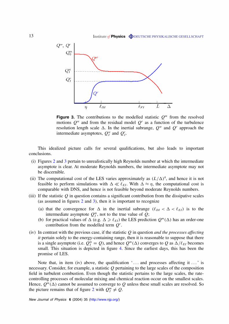
Figure 3. The contributions to the modelled statistic Qm from the resolvedmotions Qw and from the residual model Qr as a function of the turbulenceresolution length scale �. In the inertial subrange, Qw and Qr approach theintermediate asymptotes, Qw
I and QrI .
This idealized picture calls for several qualifications, but also leads to importantconclusions.
(i) Figures 2 and 3 pertain to unrealistically high Reynolds number at which the intermediateasymptote is clear. At moderate Reynolds numbers, the intermediate asymptote may notbe discernible.
(ii) The computational cost of the LES varies approximately as (L/�)4, and hence it is notfeasible to perform simulations with � � �EI . With � ≈ η, the computational cost iscomparable with DNS, and hence is not feasible beyond moderate Reynolds numbers.
(iii) If the statistic Q in question contains a significant contribution from the dissipative scales(as assumed in figures 2 and 3), then it is important to recognize
(a) that the convergence for � in the inertial subrange (�DI < � < �EI) is to theintermediate asymptote Qm
I , not to the true value of Q;(b) for practical values of � (e.g. � � �EI) the LES prediction Qm(�) has an order-one
contribution from the modelled term Qr.
(iv) In contrast with the previous case, if the statistic Q in question and the processes affectingit pertain solely to the energy-containing range, then it is reasonable to suppose that thereis a single asymptote (i.e. Qm
I = Q), and hence Qm(�) converges to Q as �/�EI becomessmall. This situation is depicted in figure 4. Since the earliest days, this has been thepromise of LES.
Note that, in item (iv) above, the qualification ‘ . . . and processes affecting it . . . ’ isnecessary. Consider, for example, a statistic Q pertaining to the large scales of the compositionfield in turbulent combustion. Even though the statistic pertains to the large scales, the rate-controlling processes of molecular mixing and chemical reaction occur on the smallest scales.Hence, Qm(�) cannot be assumed to converge to Q unless these small scales are resolved. Sothe picture remains that of figure 2 with Qm
I �= Q.
New Journal of Physics 6 (2004) 35 (http://www.njp.org/)
Figure 4. The modelled statistic Qm and its components Qw and Qr againstthe turbulence resolution length scale � for the case in which the statisticQ and the processes affecting it are confined to the energy-containingscales.
We have considered here Qm as a function of �. For adaptive LES (as described insection 5), Qm can be considered as a function of the turbulence resolution tolerance εm, andthe picture is essentially the same for Qm(εm) as it is for Qm(�).
8. What is the goal of an LES calculation?
For a given flow and a given LES model, what is the goal of the calculations performed? Thissuperficially naive question is prompted by the fact that, as discussed above, statistics Qm(�)
obtained from LES depend on the artificial parameter �. It is intrinsically unsatisfactory toaccept Qm(�) (for some value of �) as a prediction for Q—for Qm(2�) or Qm( 1
2�), forexample, may yield substantially different predictions.
A more satisfactory answer can be provided in the idealized case (considered in the previoussection) of very high Reynolds number free shear flow. The goal of the LES calculation canbe to estimate the intermediate asymptotic value Qm
I (see figure 2), which is independent of�. This can be achieved by performing LES with several (at least three) different values of �,so that the intermediate asymptote can be estimated by extrapolation to � = 0.
At moderate Reynolds number, and in more complex flows, a completely satisfactoryanswer is more elusive. However it should surely be an essential part of the LES methodologyto perform simulations over a range of � to assess the sensitivity of Qm(�) to �. If thesensitivity is large over the whole range investigated, what can be concluded about the flowstatistic Q?
9. How are different LES models to be appraised?
Given two LES models, which we refer to as model A and model B, what criteria areto be used to assess their relative merits? In the broader context of turbulence modelling
New Journal of Physics 6 (2004) 35 (http://www.njp.org/)
Figure 5. The predictions QmA(�) and QmB(�) of the statistic Q obtainedfrom LES models A and B as functions of the turbulence resolution length scale� for the case in which Q has contributions from both energy-containing anddissipative scales.
(including LES), Pope [5] suggests five criteria:
(i) level of description
(ii) completeness
(iii) cost and ease of use
(iv) range of applicability, and
(v) accuracy.
Completeness is the topic of section 5. Here we first discuss accuracy, and then cost (in conjuctionwith accuracy). For LES, an additional criterion, which we assume to be satisfied by the modelsconsidered, is convergence to DNS in the limit at �/η tends to zero.
Considering again the very high-Reynolds number flow of the previous two sections,figure 5 is a sketch of Qm(�) given by models A and B. It shows that the two models havedifferent intermediate asymptotes, denoted by QmA
I and QmBI , respectively. Recalling that the
ideal goal of an LES calculation is to estimate this intermediate asymptote, for the case depictedin figure 5, model A clearly has superior accuracy, since QmA
I is closer to Q than is QmBI . Note
that if LES calculations were performed at the single value � = �∗ then the contrary conclusionwould incorrectly be drawn.
Figure 6 depicts the situation in which the statistic Q of interest pertains solely tothe energy-containing motions and both models asymptote to Q (for �/�EI � 1). As aconsequence, each model becomes as accurate as desired as �/�EI decreases, and the criterionof accuracy alone does not favour one model over the other.
The second criterion to consider is the computational cost, most simply measured in CPUtime, T , and most simply approximated as TA = cA(L/�)4 and TB = cB(L/�)4, for models Aand B respectively, where cA and cB are model-dependent constants. Obviously the CPU timeincreases as � decreases. Figure 7 is a sketch of Qm(�) as a function of CPU time for the
New Journal of Physics 6 (2004) 35 (http://www.njp.org/)
Figure 6. The predictions QmA(�) and QmB(�) of the statistic Q obtainedfrom LES models A and B as functions of the turbulence resolution length scale� for the case in which Q and the processes affecting it are confined to theenergy-containing range.
Figure 7. For the case depicted in figure 6, QmA and QmB plotted against CPUtime T . The horizontal dashed lines show the interval of acceptable accuracy.
two models for the same case as is shown in figure 6. An error tolerance εQ is specified so thatthe calculation Qm(�) is acceptably accurate if it lies in the range [Q − εQ, Q + εQ]. For thecase depicted in figure 7, model B is superior since it achieves the required accuracy in timeT ∗
B which is less than T ∗A.
Evidently, for this case, cA is much larger than cB, i.e. for given �/L, method A is muchmore expensive. From figure 6 it is evident that, compared with method A, method B requiresa smaller value of � to achieve acceptable accuracy, yet it requires less CPU time (figure 7).
New Journal of Physics 6 (2004) 35 (http://www.njp.org/)
Thus, the principal criteria to appraise LES models are (intermediate) asymptotic accuracy,and computational cost to achieve acceptable accuracy. It is important to appreciate that such anappraisal cannot be made without characterizing the � dependence of the models. In particular,comparing models based on calculations with a single value of � can be extremely misleading.
10. Why is the dynamic model successful?
The dynamic model was proposed by Germano et al [30], with important modifications andextensions provided by Lilly [31] and Meneveau et al [32]. The model has proved quitesuccessful, and the same procedure has been applied in several other contexts.
The dynamic model is usually motivated by notions of scale similarity, although thisrationale is not explicitly stated in the original paper. If the turbulent motions possess scalesimilarity, then a model that respects this scale similarity should be applicable at differentscales (i.e. for different values of �); and this principle can be used to determine the numericalcoefficients in the model. The most well-known application is to the Smagorinsky model, inwhich the dynamic procedure is used to determine the appropriate value of the Smagorinskycoefficient cs.
Several observations cast doubt on this rationale for the dynamic Smagorinsky model:
(i) Turbulence at high Reynolds number can reasonably be assumed to possess scale similarity,but only over length scales corresponding to the inertial subrange. In the inertial subrange,the Smagorinsky model is, by construction, consistent with the known inertial-range scalinglaws, and the appropriate value of the Smagorinsky coefficient is uniquely determined (forgiven filter type) by the analysis developed by Lilly [2]. In this circumstance there is,therefore, neither need for nor benefit from the dynamic model.
(ii) It is reasonable to suppose that the Smagorinsky model yields accurate predictions ofenergy-containing statistics in high Reynolds number free flows, provided that � is wellwithin the inertial subrange. These statistics will be insensitive to a further reduction in�. In the Smagorinsky model, the coefficient cs appears only in the product cs�
2: hencedecreasing � is equivalent to decreasing cs. If energy-containing statistics are insensitiveto �, they are, therefore, also insensitive to cs, again negating the value of the dynamicprocedure.
(iii) The dynamic procedure has been most successful in remedying the standard Smagorinskymodel’s serious deficiencies in laminar flows, transitional flows and in the viscous near-wallregion. In none of these circumstances is scale similarity plausible.
(iv) Based on similar considerations, Jimenez and Moser [33] conclude that ‘the physical basisfor the good a posteriori performance of the dynamic-Smagorinsky subgrid models inLES . . . appears to be only weakly related to their ability to correctly represent the subgridphysics’.
Since the dynamic model does appear to be successful, it is natural to ask: why? Thebehaviour of the dynamic Smagorinsky model has been studied by Meneveau and Lund [34]for the case in which � approaches η, and hence scale similarity does not hold. At the otherlimit, Porte-Agel et al [35] introduce a refined dynamic procedure to produce scale-dependentcoefficients for the case in which � approaches L. In the remainder of this section, we offeran alternative principle to motivate both the standard and refined dynamic procedures.
New Journal of Physics 6 (2004) 35 (http://www.njp.org/)
As discussed in section 7, the LES prediction Qm(�) of a turbulent-flow statistic Q
pertaining to the energy-containing range (in a high-Reynolds number free flow) can be supposedto vary with � as illustrated in figure 6. The figure shows Qm(�) given by two different models,A and B, both of which converge to Q as �/�EI tends to zero. If the computational cost (atfixed �) is the same for both models, then clearly model A is superior, since it approaches theasymptote, Q, sooner as � decreases.
Another view of the same observation is provided by the identity
Qm(�) − Q = [Qm(�I) − Q] +∫ �
�I
dQm(�)
d�d�, (11)
which follows from the fundamental theorem of calculus (for any differentiable function Qm(�)).The left-hand side represents the error in the LES prediction as a function of �, which we requireit to be as small as possible (in magnitude). The first term on the right-hand side representsthe error in the prediction for � = �I , and we take �I to be sufficiently small for this errorto be negligible. Thus the error (at scale �) is essentially given by the last term; and, roughlyspeaking, the smaller the derivative |dQm(�)/d�|, the smaller the error. As may be seen fromfigure 6, the derivative |dQm(�)/d�| is smaller for method A compared with method B.
Based on this observation, it is natural to seek an LES model which has the followingproperties (with respect to statistics Qm(�) of interest pertaining to the energy-containingmotions in a high-Reynolds number flow):
(a) for � = �I well within the inertial subrange, the LES predictions are accurate,
(b) for � > �I , the predicted statistics vary as weakly as possible with �.
We suppose that (a) is satisfied by any reasonable model that has the correct inertial-rangescaling (e.g. the Smagorinsky model), and so we focus on property (b).
The dynamic model is based on filtering. Specifically, it is based on quantities filtered withrespect to one filter of width �, and a second filter of somewhat larger width �. Quantities so
filtered are denoted by, for example, U and U, respectively. The LES model Qm for the statisticQ of interest can be evaluated based on U and �, i.e.
Qm(�) = Qw(U) + Qr(U, �), (12)
where Qw denotes the contribution from the resolved motions (determined solely from U), andQr is the model for the contribution from the residual motions. For the same statistic Q, theLES model can also be applied based on U and �, i.e.
Qm(�) = Qw(U) + Qr(U, �). (13)
To fulfil condition (b), we introduce the following principle: the LES model coefficients
should be chosen to minimize the difference between Qm(�) and Qm(�).As depicted in figure 4, as � decreases from � ≈ L, Qw increases, whereas Qr decreases.
The magnitude of Qr is typically proportional to a model constant, cQ, say. An interpretationof the above principle is that cQ should be chosen so that the decrease in Qr(�) as � decreases
from � to � should be balanced by the corresponding increase in Qw(�). Figure 8 illustrates
New Journal of Physics 6 (2004) 35 (http://www.njp.org/)
Figure 8. For the given model A, and the dynamic model D, a sketch of theresolved contribution Qw(�) and of the modelled residual contributions QrA(�)
and QrD(�) to the model predictions QmA(�) and QmD(�) of a large-scalestatistic Q. The dynamic model selects the model coefficient cQ so that QmD(�)
equals QmD(�).
these ideas for a model denoted by A with a fixed value of cQ, and for the dynamic modeldenoted by D. (For simplicity, the resolved contribution Qw is taken to be the same for bothmodels.) As may be seen from the figure, for model A, the decrease in Qr, i.e. QrA(�) − QrA(�)
is less than the increase in Qw, i.e. Qw(�) − Qw(�), and consequently the model predictionQmA(�) is less than QmA(�). According to the above principle, the value of cQ is too small
in model A. The dynamic procedure selects cQ so that QmD(�) equals QmD(�).We now apply this principle to the Smagorinsky model and show that it yields essentially
the same specification for the Smagorinsky coefficient cs as the dynamic procedure. The LESequations incorporating the Smagorinsky model are solved with � = �. The resolved velocityfield W(x, t) is deemed to model the filtered velocity field U(x, t).
The LES field W is filtered with a filter of width �, so that W corresponds to the doubly
filtered velocity field U. The filter width � is that corresponding to filtering by � and then by�: for a Gaussian filter the relation is � = [�2 + �2]1/2. Thus, it is assumed (as in the standarddynamic model) that the statistics of the LES fields W and W are the same as those of the
filtered fields U and U.We consider the quantity
Qij(x, t, �) ≡ UiUj − 13UkUkδij, (14)
defined at the � filter level. The corresponding quantity at the � filter level is consistentlydefined by
Qij(�) ≡ UiUj − 13UkUkδij, (15)
New Journal of Physics 6 (2004) 35 (http://www.njp.org/)
where the dependence on x and t is no longer shown explicitly. It is readily observed that thesetwo quantities are related by
Qij(�) = Qij(�). (16)
The Smagorinsky model for Qij(�), denoted by Qmij (�), can be written as
Qmij (�) = Qw
ij(�) + Qrij(�), (17)
where
Qwij(�) ≡ UiUj − 1
3UkUkδij (18)
is the contribution that is known from the resolved field, and
Qrij(�) ≡ −2cs(�)�2S Sij (19)
is the Smagorinsky model for the residual contribution. Here cs(�) is the Smagorinsky coefficientat scale �; Sij is the filtered rate of strain
Sij ≡ 1
2
(∂Ui
∂xj
+∂Uj
∂xi
), (20)
and S is the filtered rate-of-strain invariant
S ≡ [2SijSij]1/2. (21)
The same model applied at the � filter level is
Qmij (�) = Qw
ij(�) + Qrij(�), (22)
where Qwij(�) and Qr
ij(�) are defined analogously to equations (18) and (19), with the latter
involving the coefficient cs(�).In view of the identity, equation (16), these model equations provide two estimates of
Qij(�): the first is directly in terms of U from equation (22); the second is from filteringequation (17) which is based on U, i.e.
Qmij (�) = Qw
ij (�) + Qrij(�). (23)
We are now in a position to state, in this context, the alternative principle that leads tothe dynamic model. This principle is: the model coefficient cs should be chosen to minimize
the mean-square difference between the model’s prediction of Qij(�) based on U, equation(22), and that based on U , equation (23). Note that there is no appeal to the scale similarity.
New Journal of Physics 6 (2004) 35 (http://www.njp.org/)
Rather, the aim is to select cs so that the statistics predicted at a single filter level (i.e. Qij(�))
depend as little as possible on the level of the filtered velocity field (i.e. U or U) on which theprediction is based.
The difference to be minimized is
δQmij ≡ Qm
ij (�) − Qmij (�). (24)
This is obtained by subtracting equation (23) from equation (22), and in the notation of Pope[5] the result is
δQmij = Ld
ij − cs(�)Mij, (25)
with the definitions
Ldij ≡ (Ui Uj − 1
3Uk Ukδij) − (Ui Uj − 13Uk Ukδij), (26)
Mij ≡ 2γ�2S Sij − 2�2S Sij (27)
and
γ ≡ cs(�)/cs(�). (28)
(As in the usual derivation of the dynamic model, equation (25) involves the approximationthat, when equation (19) is filtered, cs(�) is taken to be spatially uniform.)
The unknown parameter γ is unity if scale similarity prevails, and is close to unity otherwise.For the usual case (�)/� = 2, the second term in equation (27) is approximately 4 times thefirst term, and hence the value of cs(�) is insensitive to γ . Thus, the standard practice of settingγ = 1 is a reasonable first approximation, even when scale similarity does not hold.
The mean-square difference between the two predictions of Qmij (�) is
χ ≡ 〈δQmij δQ
mij 〉. (29)
It follows simply from equation (25) that the value of cs(�) which minimizes χ is
c∗s ≡ 〈Ld
ijMij〉/〈MijMij〉. (30)
This is just the standard formula for cs used in the dynamic model, except that some practicalform of averaging is used, rather than using expectations.
As observed by Porte-Agel et al [35], this dynamic procedure yields (to a firstapproximation) the value of the Smagorinsky coefficient cs(�) at the scale �, whereas, toperform the LES, the value of cs(�) is required. Hence a refined procedure, such as thatadvanced by Porte-Agel et al [35], provides an estimate of γ to be used in equation (27), and,more importantly, so that cs at the required scale is obtained as cs(�) = γcs(�).
For the simplest case of high-Reynolds number homogenous isotropic turbulence, thedynamic procedure can be applied to determine c∗
s as a function of � (for fixed �/�). For �
New Journal of Physics 6 (2004) 35 (http://www.njp.org/)
in the inertial subrange, one expects c∗s to be independent of �, and equal to the value given by
the Lilly analysis. But as � increases beyond �EI towards the integral scale L, the expectationis that c∗
s decreases. Thus, in the inertial subrange the Smagorinsky length scale �s, defined
by �2s ≡ c∗
s �2, varies as � in accord with inertial range scaling; however, for larger values of
�, �s increases more slowly than � (as c∗s decreases).
In summary, it has been shown that both the standard and refined dynamic procedurescan be derived from the principle that the model coefficients should be chosen (as functionsof �) to minimize the dependence of relevant turbulence statistics on �. In particular, for theSmagorinsky model, the coefficient cs(�) is chosen to minimize the difference between Qij(�),
equation (15), evaluated based on U and on U. If scale similarity holds then γ is unity, andthe procedure yields the standard result for cs(�) = cs(�). If scale similarity does not hold,then (setting γ = 1), the procedure yields a reasonable approximation to cs(�). In a refinedprocedure, the value of γ is estimated so as to provide an improved estimate of cs(�) and,more importantly, of cs(�) = cs(�).
11. Conclusions
As we enter the era in which there is sufficient computer power for LES, it is useful to re-examine both the conceptual foundations of the approach and the methodologies and protocolsgenerally employed.
For flows in which rate-controlling processes occur below the resolved scales (e.g. near-wall flows and combustion), LES calculations have a first-order dependence on the modellingof these processes. Approaches that include a statistical resolution of all scales provide a morefundamental description of the rate-controlling processes; however, it remains a challenge todevise such approaches that are computationally tractable and free of empiricism.
The relationship between the resolved LES velocity field W(x, t) and the turbulent velocityfield U(x, t) can only be statistical. Corresponding to a turbulence statistic Q, the LES providesa model Qm for Q of the form
Qm = Qw + Qr, (31)
where Qw is the contribution from the resolved motions (which is obtained directly from W )and Qr is the modelled contribution from the residual motions.
In LES, the turbulence resolution length scale �(x) is an artificial parameter of primeimportance. As a rule, as � decreases, Qw increases and Qr decreases. Unless demonstratedotherwise, there is every reason to suppose that LES predictions Qm depend (maybe strongly)on �. As a consequence, characterizing the dependence of predictions on � must be part ofthe overall LES methodology.
As currently practised, LES is incomplete because the turbulence resolution length scale�(x) is specified subjectively in a flow-dependent manner. It can be made complete throughadaptive LES. The variation of �(x, t) is controlled (by grid adaption) so that a measure M(x, t)
of turbulence resolution (e.g. the fraction of the turbulent kinetic energy in the resolved motions)is everywhere below a specified tolerance εM .
New Journal of Physics 6 (2004) 35 (http://www.njp.org/)
In a high-Reynolds-number turbulent flow, as � is decreased into the inertial subrange,it can be supposed that Qw and Qr approach an intermediate asymptote (provided that themodel is consistent with inertial-range scaling). As � is decreased through the dissipationrange, Qm approaches the correct value Q (provided that the model appropriately reverts to theNavier–Stokes equations in this limit). The most that an LES calculation can hope to achieve,is to obtain an accurate estimate of the intermediate asymptote Qm
I . This asymptote may ormay not be equal to Q depending upon whether or not Q and the processes affecting it dependsolely on the energy-containing scales.
With respect to the criteria ‘accuracy’and ‘cost’, the relative merits of different LES modelscan be appraised only when the dependence of their predictions on � has been characterized.If the intermediate asymptote Qm
I differs from the turbulence statistic Q, then the model whosevalue of Qm
I is closest to Q is to be preferred, based on the criterion of accuracy. If severalmodels have Q as their intermediate asymptote, then the model which achieves acceptableaccuracy with the least computational cost is to be preferred. By this criterion, it is highlyprobable that the optimal model contains non-negligible numerical errors.
An alternative principle is advanced to justify the dynamic procedure, namely, the LESmodel coefficients should be chosen to minimize the difference between Qm(�) and Qm(�)
(where � is the value of � used in the LES and � is somewhat larger). It is shown thatthis principle applied to the Smagorinsky model results in essentially the same formula forthe coefficient cs (i.e. equation (30)) as the standard dynamic model. As previously observedby Porte-Agel et al [35], if scale similarity does not hold, then the coefficient obtained is anapproximation to the appropriate value at scale �, not at the required scale �.
Acknowledgments
I am grateful to D A Caughey, R O Fox, D C Haworth, J C R Hunt, A Lamorgese, C Meneveau,R D Moser, B Vreman and Z Warhaft for valuable comments on a draft of this paper. This workis supported by the Air Force Office of Scientific Research under Grant No. F-49620-00-1-0171.
References
[1] Smagorinsky J 1963 Mon. Weather Rev. 91 99[2] Lilly D K 1967 The representation of small-scale turbulence in numerical simulation experiments
Proc. IBM Scientific Computing Symp. on Environmental Sciences (Yorktown Heights, New York) edH H Goldstine, IBM form no. 320-1951, p 195
[3] Deardorff J W 1974 Boundary-Layer Meteorol. 7 81[4] Schumann U 1975 J. Comput. Phys. 18 376[5] Pope S B 2000 Turbulent Flows (Cambridge: Cambridge University Press)[6] Sagaut P 2001 Large Eddy Simulation for Incompressible Flows (Berlin: Springer)[7] Rogallo R S and Moin P 1985 Ann. Rev. Fluid Mech. 17 99[8] Galperin B and Orszag S A 1993 Large Eddy Simulation of Complex Engineering and Geophysical Flows
(Cambridge: Cambridge University Press)[9] Lesieur M and Metais O 1996 Ann. Rev. Fluid Mech. 28 45
[10] Meneveau C and Katz J 2000 Ann. Rev. Fluid Mech. 32 1[11] Leonard A 1974 Adv. Geophys. 18A 237[12] Boris J P, Grinstein F F, Oran E S and Kolbe R L 1992 Fluid Dyn. Res. 10 199
New Journal of Physics 6 (2004) 35 (http://www.njp.org/)
[13] Pope S B 1999 A perspective on turbulence modeling Modeling Complex Turbulent Flows ed M D Salas,J N Hefner and L Sakell (Dordrecht: Kluwer) p 53
[14] Peters N 2000 Turbulent Combustion (Cambridge: Cambridge University Press)[15] Chapman D R 1979 AIAA J. 17 1293[16] Meneguzzi M, Politano H, Pouquet A and Zolver M 1996 J. Comput. Phys. 123 32[17] Kerstein A R 1988 Combust. Sci. Technol. 60 391[18] Kerstein A R 1999 J. Fluid Mech. 392 277[19] Menon S, McMurtry P A and Kerstein A R 1993 A linear eddy mixing model for large-eddy simulation of
turbulent combustion LES of Complex Engineering and Geophysical Flows ed B Galperin and S Orszag(Cambridge: Cambridge University Press)
[20] Sankaran V and Menon S 2000 Proc. Combust. Inst. 28 203[21] Reynolds W C 1990 The potential and limitations of direct and large eddy simulations Whither Turbulence?
Turbulence at the Crossroads (Lecture Notes in Physics vol 357) ed J L Lumley (Berlin: Springer)p 313
[22] Vreman B, Geurts B and Kuerten H 1996 Int. J. Numer. Meth. Fluids 22 297[23] Meyers J, Geurts B J and Baelmans M 2003 Phys. Fluids 15 2740[24] Langford J A and Moser R D 1999 J. Fluid Mech. 398 321[25] Pope S B 2001 Large-eddy simulation using projection onto local basis functions Fluid Mechanics and
the Environment: Dynamical Approaches ed J L Lumley (Berlin: Springer) p 239[26] Kravchenko A G and Moin P 1997 J. Comput. Phys. 131 310[27] Lesieur M 1990 Turbulence in Fluids 2nd edn (Dordrecht: Kluwer)[28] Vreman B, Geurts B and Kuerten H 1997 J. Fluid Mech. 339 357[29] Chow F K and Moin P 2003 J. Comput. Phys. 184 366[30] Germano M, Piomelli U, Moin P and Cabot W H 1991 Phys. Fluids A 3 1760[31] Lilly D K 1992 Phys. Fluids A 4 633[32] Meneveau C, Lund T S and Cabot W H 1996 J. Fluid Mech. 319 353[33] Jimenez J and Moser R D 1998 AIAA Paper 98-2891[34] Meneveau C and Lund T S 1997 Phys. Fluids 9 3932[35] Porte-Agel F, Meneveau C and Parlange M B 2000 J. Fluid Mech. 415 261
New Journal of Physics 6 (2004) 35 (http://www.njp.org/)