Page 1
SAMPLED-DATA CONTROL BASED ON DISCRETE-TIME
EQUIVALENT MODELS
By
FAHAD MUMTAZ MALIK
A DISSERTATION
Submitted to
National University of Sciences and Technology
in partial fulfillment of the requirements for the degree of
DOCTOR OF PHILOSOPHY
Supervised by
DR MOHAMMAD BILAL MALIK
College of Electrical and Mechanical Engineering
National University of Sciences and Technology, Pakistan
2009
Page 2
ii
In the name of Allah, the most Merciful and the most Beneficent
Page 3
iii
ABSTRACT
SAMPLED-DATA CONTROL BASED ON DISCRETE-TIME
EQUIVALENT MODELS
By
FAHAD MUMTAZ MALIK
This thesis focuses on the design and performance of sampled-data control of
continuous-time systems. The philosophy of the control law design is based on
stabilization of discrete-time equivalent models of the continuous-time system. The
development in the thesis can be broadly classified into sampled-data stabilization of a
class of underactuated linear systems and sampled-data stabilization of locally Lipschitz
nonlinear systems.
The class of underactuated linear systems considered in the thesis has time
varying actuation characteristics. The system can be actuated with a short duration pulse
during a fixed interval of time. The system is unactuated otherwise in the interval. Based
on these actuation characteristics, a discrete-time equivalent model can be developed by
integrating the continuous-time model. The equivalent model is time invariant and fully
actuated thus discrete-time control law design for sampled-data control is facilitated.
The closed form exact discrete-time equivalent model (obtained by integrating the
continuous-time model over the sampling interval) cannot be obtained for nonlinear
systems in general. As an alternative, the continuous-time model is discretized using the
Euler method. Discretization using the Euler method has an associated discretization
Page 4
iv
error. This error may become unbounded in certain cases for nonlinear systems. This
provides the motivation for analysis of discretization error bounds for nonlinear systems.
Analyses show that locally Lipschitz nonlinear systems discretized using the Euler
method have bounded discretization error for sampling time less than the guaranteed
interval of existence. The error bound is a function of Lipschitz constant and sampling
time.
The discrete-time control law is designed on the basis of system model discretized
using the Euler method. The sampled-data closed loop performance of locally Lipschitz
nonlinear systems is analyzed using discretization error bounds and Lyapunov method.
Locally Lipschitz nonlinear systems with state feedback control are analyzed in general
whereas performance of output feedback control using discrete-time observers is
investigated for a sub-class of locally Lipschitz nonlinear systems.
Asymptotic/exponential stability of closed loop sampled-data systems is established for
arbitrarily small sampling time; moreover it is shown that asymptotic/exponential
stability can be achieved for nonzero sampling time under some additional conditions.
The results are demonstrated by sampled-data control of nonlinear systems.
Page 5
v
To my beloved
Islamic Republic of Pakistan
Page 6
vi
ACKNOWLEDGEMENTS
All praises and thanks are due to, Allah Almighty, the Lord of the Universe, for
His merciful and divine direction throughout my study. Afterwards, I would like to
acknowledge the guidance and cooperation of all my teachers whose earnest efforts have
made possible the successful completion of this work. In particular, my MS and PhD
supervisor Dr Mohammad Bilal Malik, who not only extensively guided me throughout
the course of my postgraduate studies but also provided tremendous moral support and
inspiration.
I would like to express my sincere gratitude to my GEC member Dr Mohammad
Ali Maud, Dr Ejaz Muhammad and Dr Khalid Munawar for their precious time and
guidance that I have received from them. In particular Dr. Khalid Munawar who always
gave me his gentle and kind attention whenever I desired so. I would address special
thanks to Dr Muhammad Salman Masaud who as a senior always selflessly helped and
supported me. I would also thank my colleagues Muhammad Asim Ajaz, Aamir Hussain,
Usman Ali and Saqib Mehmood for their cooperation and beneficial academic
discussions I have had with them.
I am grateful to my father Muhammad Mumtaz Khan, my mother and my elder
brother Shahid Mumtaz Malik who always supported and encouraged me throughout my
life. I would also like to thank my dear friends Syed Khurram Mehmood and Anees
Mumtaz Abbasi for motivating me and keeping me in a positive state of mind. I am
Page 7
vii
indebted to my wife who has been very supportive and has shown extraordinary patience
towards the later half of this work.
I would also like to gratefully acknowledge National University of Sciences and
Technology, Pakistan for the financial support it provided for my studies and research.
Page 8
viii
TABLE OF CONTENTS
CHAPTER 1 INTRODUCTION ................................................................................... 1
1.1 Sampled-Data Control ..........................................................................................1
1.2 Control law Design….. .........................................................................................2
1.3 Class of Underactuated Linear Systems ...............................................................6
1.4 Locally Lipschitz Nonlinear Systems ...................................................................7
1.5 The Need for New Developments.......................................................................12
1.6 Contribution of the Thesis ..................................................................................13
1.7 Overview of the Thesis .......................................................................................14
CHAPTER 2 SAMPLED-DATA STABILIZATION OF UNDERACTUATED
LINEAR SYSTEMS.............................................................................. 16
2.1 Continuous-Time Underactuated Linear System................................................17
2.2 Discrete-Time Equivalent Model........................................................................18
2.3 Discrete-time Controller .....................................................................................20
2.4 System with Delayed Input.................................................................................22
2.5 Example: The Underactuated Drill Machine ......................................................26
2.6 Summary…………….. .......................................................................................38
CHAPTER 3 DISCRETIZATION ERROR BOUNDS FOR NONLINEAR SYSTEMS
................................................................................................................ 39
Page 9
ix
3.1 Single-Step Input Discretization Error Bound....................................................40
3.2 Single-Step Model Discretization Error Bound..................................................47
3.3 Multi-Step Input Discretization Error Bound .....................................................50
3.4 Multi-Step Model Discretization Error Bound ...................................................57
3.5 Examples…………….........................................................................................62
3.6 Summary…………….. .......................................................................................68
CHAPTER 4 SAMPLED-DATA STATE FEEDBACK STABILIZATION OF
NONLINEAR SYSTEMS ..................................................................... 69
4.1 Continuous-time Nonlinear System....................................................................70
4.2 Discrete-time Control Law .................................................................................72
4.3 Convergence Analyses ............…………………………………………………74
4.4 Feedback Linearizable Systems..........................................................................97
4.5 Examples…………….........................................................................................99
4.6 Summary…………….. .....................................................................................104
CHAPTER 5 SAMPLED-DATA OUTPUT FEEDBACK STABILIZTION OF
NONLINEAR SYSTEMS ................................................................... 105
5.1 The Class of Continuous-Time Nonlinear Systems..........................................105
5.2 Discrete-time Output Feedback Control Law...................................................107
5.3 Convergence Analyses......................................................................................112
5.4 Examples…………….......................................................................................140
5.5 Summary…………….. .....................................................................................145
CHAPTER 6 CONCLUSIONS AND FUTURE SUGGESTIONS........................... 146
6.1 Conclusions………….......................................................................................146
Page 10
x
6.2 Future Suggestions…………............................................................................148
References……............................................................................................................... 150
Page 11
xi
LIST OF FIGURES
Figure 1-1. Sampled-data Control....................................................................................... 1
Figure 2-1. Single Actuation Cycle of Period L ............................................................... 18
Figure 2-2. Construction of the Underactuated Drill Machine ......................................... 28
Figure 2-3. Position of Actuation...................................................................................... 30
Figure 2-4. Stabilization of the Drill Bit without Input Delay.......................................... 36
Figure 2-5. Stabilization of the Drill Bit with Input Delay of a Single Sample ............... 37
Figure 3-1. Discretization Error and its Bounds for T=0.03s ........................................... 64
Figure 3-2. Discretization Error and its Specified Bound for Variable Sampling Time .. 66
Figure 3-3. Discretization Error and its Bounds for Saturation Function........................ 67
Figure 4-1. Illustration of Ultimate Boundedness............................................................. 75
Figure 4-2. Geometrical Representation of Sets for Illustration of Ultimate Boundedness
................................................................................................................................... 76
Figure 4-3. Illustration of Trajectory Convergence .......................................................... 78
Figure 4-4. Exponential Stabilization of Inverted Pendulum ......................................... 101
Figure 4-5. Exponential Stabilization of Manipulator with Flexible Joints.................... 103
Figure 5-1. Geometrical Representation of Sets for Illustration of Boundedness .......... 114
Figure 5-2. Stabilization of Inverted Pendulum.............................................................. 141
Figure 5-3. Estimated States of Pendulum Using Discrete-Time Observer .................. 142
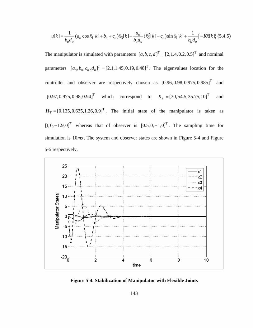
Figure 5-4. Stabilization of Manipulator with Flexible Joints........................................ 143
Page 12
xii
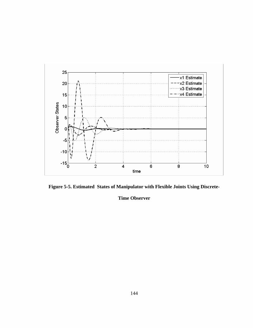
Figure 5-5. Estimated States of Manipulator with Flexible Joints Using Discrete-Time
Observer.................................................................................................................. 144
Page 13
xiii
LIST OF TABLES
Table 3-1. Escape Time Corresponding to Different Sampling Times ............................ 62
Page 14
1
CHAPTER 1
INTRODUCTION
1.1 Sampled-Data Control
Control of a continuous-time system by a digital controller is termed as sampled-
data control [13], [21], [32], [34], [38]. The digital controller (typically a microcontroller)
is fed with discretized states or output of the continuous-time system. The states or output
is discretized using a sample and hold circuit. The controller determines the input for the
continuous-time system using the states/output according to a discrete-time control law.
This discrete control input is then applied to the continuous-time system via a zero-order-
hold circuit [33]. The concept of sampled-data control is illustrated in Figure 1-1 ([60],
[61]).
Figure 1-1. Sampled-data Control
D/A Converter
Continuous-time System
A/D Converter
Discrete Reference
States /Output
Discrete-time control input
Digital Controller
Page 15
2
The use of microcontrollers has virtually eliminated analog electronics in the
control of continuous-time systems. The popularity of microcontrollers is attributed to
their computational power and convenience of use. More recently, faster sampling rates
and enhanced computational power of DSP microcontrollers has enabled the
implementation of sophisticated control schemes related to control systems.
The qualitative properties of sampled-data systems have been studied by many
researchers. A few noteworthy contributions include the study of quantization effects on
the stability of closed loop sampled-data system by L. Hou, A. N. Michel and H. Ye in
[41] and by R. K. Miller, A. N. Michel and coworkers in [65], [66] . Robustness of
sampled data systems to measurement noise, computational delays and fast actuator
dynamics is established by C. Kellet, M. Shim and A. R. Teel using Lyapunov analysis in
[48]. Some other important contributions are [42] and [78].
1.2 Control law Design
Control law for any system is designed on the basis of mathematical model of the
system that describes its dynamical behavior. The mathematical model for a continuous-
time system is typically a set of differential equations. A large class of physical systems
can be modeled using state space representation, which is a set of first order differential
equations. The emphasis of modern development in the area of control systems is on state
space representation.
The mathematical model of a continuous-time system written in state space is
( , )x f x u= , (1.2.1)
Page 16
3
where nx R∈ is the n dimensional state of the system, mu R∈ is the m dimensional
input and x represents the derivative of the state vector with respect to time. The
function f represents the map of states and input to the derivatives of the states.
Consider that (1.2.1) is to be controlled in sampled-data form with sampling time
T . In order to design a discrete-time control law for this purpose, a discrete-time model
of (1.2.1) with sampling time T is required. An exact discrete-time equivalent model will
be the solution of set of differential equations (1.2.1) over the interval [ , ( 1) ]t kT k T∈ + ,
where k is an arbitrary integer. Let the state of (1.2.1) at time t kT= be ( )x kT , then the
state at time ( 1)t k T= + using fundamental theorem of calculus [35] is
( 1)
( 1) ( ) ( ( ), ( ))k T
kT
x k T x kT f x u dτ τ τ+
+ = + ∫ . (1.2.2)
The input ( )u t is zero-order-held in case of sampled-data systems. Mathematically,
( ) ( ) [ , ( 1) ]u t u kT t kT k T= ∀ ∈ + . (1.2.3)
Using (1.2.3), equation (1.2.1) can be written as
( 1)
( 1) ( ) ( ( ), ( ))k T
kT
x k T x kT f x u kT dτ τ+
+ = + ∫ . (1.2.4)
The discrete-time model (1.2.4) is termed as exact discrete-time model ([3], [12]) for the
system (1.2.1) with zero-order-held input. The discrete-time control law for the sampled-
data control of continuous-time system (1.2.1) is designed on the basis of exact discrete-
time model (1.2.4).
Page 17
4
1.2.1 Linear Time Invariant Systems
The closed form exact discrete-time model with zero-order-held input can be
easily obtained for linear time invariant systems using integration. To illustrate this
concept consider the following LTI system
x Ax Bu= + , (1.2.5)
where A and B are time invariant matrices that represent the map of states and input
respectively to the derivative of states. The exact discrete-time model for (1.2.5) with
sampling time T is given by
( )
( )
( ) exp( ( )) ( ) exp ( ) ( )
exp( ) ( ) exp ( ) ( )
kT T
kTkT T
kT
x kT T A kT T kT x kT A kT T Bu kT d
AT x kT A kT T d Bu kT
σ σ
σ σ
+
+
+ = + − + + −
= + + −
∫
∫(1.2.6)
Using change of variables it can be shown that
( )0
( ) exp( ) ( ) exp ( ) ( )T
x kT T AT x kT A T d Bu kTσ σ+ = + −∫ . (1.2.7)
Hence the exact discrete-time model for (1.2.5) can be written as
( ) ( ) ( )d dx kT T A x kT B u kT+ = + , (1.2.8)
where ( )0
exp( )and exp ( )T
d dA AT B A T d Bσ σ= = −∫ .
The discrete-time control law that stabilizes (1.2.8) can be easily designed.
In this thesis a discrete-time control scheme is proposed for a class of
underactuated linear systems based on the corresponding exact discrete-time model.
Page 18
5
1.2.2 Nonlinear Systems
In the case of nonlinear systems, the closed form exact discrete-time model
(1.2.4) cannot be obtained in general. To overcome this problem the following two
logical approaches have been adopted by researchers to design discrete-time control law
for the stabilization of nonlinear systems in sampled-data form.
1. Continuous-time control law is designed that stabilizes the continuous-time nonlinear
system model. This control law is then discretized according to the sampling time and
implemented in sampled-data form.
2. The continuous-time system model is discretized according to the sampling time
using numerical techniques. The resulting discrete-time model is termed as
approximate discrete-time model. Discrete-time control law is then designed that
stabilizes the approximate discrete-time model.
The first approach for control law design is well established and is widely
practiced by control engineers [56], [79], [83]. Many researchers have investigated the
performance of closed loop sampled-data nonlinear systems with control law designed
using this approach. A few pertinent contributions are [19], [22], [25] and [82].
The second approach for control law design is relatively new and less recognized.
However this approach has certain advantages over the first one, for example, the
resulting closed loop system has a larger region of attraction with this design approach as
compared with the first one for equal sampling time. The superiority of this approach is
attributed to the fact that the approximate discrete-time model is better at approximating
the exact discrete-time model as compared to the continuous-time system [70].
Page 19
6
In this thesis, the performance of state and output feedback discrete-time control
law designed for a class of nonlinear systems using the second approach is analyzed.
1.3 Class of Underactuated Linear Systems
An area of contemporary research in control systems is the control of
underactuated systems. Underactuated systems have more degrees of freedom than the
number of control inputs. The significance of underactuated systems is attributed to the
fact that many sophisticated engineering systems ranging from robotic manipulators to
hovercrafts and spacecrafts are underactuated. The dynamics of underactuated system are
usually subject to nonholonomic constraints; wherein these constraints are time invariant
In the vast literature on underactuated systems, many contributions can be found
on the control law design and closed loop analysis of systems with nonholonomic
constraints. Stabilization of systems with first order nonholonomic constraints is
discussed in [15], [53] and that of systems with second order nonholonomic constraints is
presented in [75], while their tracking problem is addressed in [2]. On the other hand, the
performance of internally stabilizing feedback controllers for linear time invariant MIMO
underactuated systems is investigated in [84].
In this thesis a class of underactuated linear systems is considered. The
underactuation of this class of systems is different from the underactuation of systems
generally discussed in literature. Certain electromagnetically actuated mechanical
systems belong to this class. The system can be periodically actuated with a short
duration pulse during a fixed interval of time known as actuation cycle. The system is
unactuated for the remaining time during the cycle. The phase of pulse depends upon the
desired reference for stabilization and has to be determined online by the controller. In
Page 20
7
simple words the actuation characteristics are time varying, i.e the system is fully
actuated for a short duration and unactuated otherwise. The special underactuation of the
class of systems longs for the development of a novel control scheme.
1.4 Locally Lipschitz Nonlinear Systems
In this thesis, the performance of control law designed on the basis of
approximate discrete-time model of nonlinear systems is analyzed. The continuous-time
system is assumed to be locally Lipschitz over the domain of interest. Moreover
discretization of the nonlinear system is carried out using the famous Forward difference
or Euler method.
Consider that (1.2.1) is a nonlinear system. A nonlinear system is locally
Lipschitz in state x at ox x= if it satisfies the following condition [49]
( ) ( ) 1, , , xf x u f y u L x y x y B− ≤ − ∀ ∈ , (1.4.1)
where
{ }x o xB x x x r= − ≤ (1.4.2)
and 1L is the Lipschitz constant for ( , )f x u in x .
The discretization of the nonlinear system (1.2.1) is carried out using the forward
difference or Euler method, since it is a well suited discretization tool from the
perspective of control law design as it preserves the structure of the continuous-time
system [72]. The performance of various control techniques based on the Euler
discretized system model has been explored in the past in adaptive control [29], [64], [77]
and backstepping control [71].
Page 21
8
The performance of discrete-time control based on approximate discrete-time
models using the Euler method depends tremendously on the characteristics of the
discretization error. The discretization error is the difference between the states of exact
and approximate discrete-time models. Discretization using forward difference method
may result in large discretization error (which may even become unbounded in certain
cases [58]). This can be attributed to phenomena like finite escape time which are
specific to nonlinear systems. Therefore it is imperative to investigate the difference in
the dynamical behavior of the actual nonlinear system and its discrete-time
approximation.
An important concept that needs to be explained before proceeding to the
historical developments for the analysis of the discretization error is that the
discretization of a system is a two step procedure. In the first step, the input to the system
is considered to be held constant during the sampling interval (zero-order-held). In the
second step the continuous-time system model with zero-order-held input is discretized.
The errors associated with both of these steps are referred to in this thesis as input
discretization error and model discretization error respectively. In the case of sampled-
data control, the input is applied to the system via a zero order hold thus input
discretization error has no role and the net discretization error reduces to the model
discretization error alone. The input discretization error bound analysis is useful for
comparing the performance of nonlinear system with zero-order-held inputs and
continuous inputs.
Page 22
9
The conventional discretization error bound analyses can be classified into two
categories based on Lipschitz properties of nonlinear systems. For globally Lipschitz
nonlinear systems having bounded second order derivative over the interval of interest,
the discretization error bound is derived using the Taylor series expansion. These
analyses can be found in numerous numerical analysis text books such as [7], [11], [17],
[40], [54], [68] and references therein. However the global Lipschitz condition and
bounded second order derivative requirements restrict the application of these analyses.
Discretization error bounds for locally Lipschitz nonlinear systems can be found
in [37] (section 1.7). The same has also been discussed by Nesic, Teel and Kokotovic in
[70] as single and multi-step modeling consistency and included locally Lipschitz
systems as a special case. The analyses presented in these contributions are based on
certain system properties which results in loose discretization error bounds. For instance,
discretization error bound derived in [37] requires a bound on the nonlinear function in a
neighborhood of the solution.
The stability analysis of discrete-time nonlinear systems has been discussed in
[46], [85] and [86]. The performance of the control law designed on the basis of
approximate discrete-time model for nonlinear systems in general has been analyzed by
Nesic and Teel in their contributions [69], [70], [73] and [74]. In these papers, they have
established that if the discrete-time control law asymptotically stabilizes (states tend to
zero as time tends to infinity) the approximate discrete-time model, then under sufficient
conditions, the exact discrete-time model is practically asymptotically stabilized. The
concept of practical stability is that the states of exact discrete-time model remain
Page 23
10
bounded, where they decreases asymptotically but remains nonzero even as time tends to
infinity. The sufficient conditions are
• Modeling consistency (exact and approximate discrete-time model converge as
sampling time approaches zero).
• Uniformly bounded control law.
• Existence of a continuous Lyapunov function for the closed loop approximate
model.
The analyses of Nesic and Teel provide a broad framework for stabilization of
sampled-data nonlinear systems based on approximate discrete-time model. However, the
design and in-depth analysis of control laws for various classes of nonlinear systems
using this approach was left as an open area of significant research.
In this thesis the, performance of output feedback control law for the following
sub-class of locally Lipschitz single input, single output (SISO) nonlinear systems based
on approximate discrete-time model is also analyzed.
( , )c c
c
x A x B x uy C x
φ= +
= (1.4.3)
where nx R∈ is the state u R∈ is the input and y R∈ is the output. The function (.,.)φ
is nonlinear and locally Lipschitz in its arguments. The canonical matrices cA , cB and
cC are defined as follows
Page 24
11
0 1 0 0 00 0 0
,1
0 0 0 1[1 0 ... ... 0]
c c
c
A B
C
⎡ ⎤ ⎡ ⎤⎢ ⎥ ⎢ ⎥⎢ ⎥ ⎢ ⎥= =⎢ ⎥ ⎢ ⎥⎢ ⎥ ⎢ ⎥⎣ ⎦ ⎣ ⎦
=
(1.4.4)
A variety of mechanical/electromechanical system and feedback linearizable
nonlinear systems are modeled by (1.4.3) ([4], [31], [43], [51]). The control law and
observer both are designed on the basis of approximate discrete-time model.
In case of output feedback control, observers are used for state estimation [14],
[44], [57]. Design and performance analysis of observers for discrete-time nonlinear
systems in general, can be found in [18], [50], [88] and [90]. The design of a discrete-
time observer based on the approximate discrete-time model of a continuous-time
nonlinear system has been explored in [8], [9], and [72]. In [72], Nesic and Teel analyzed
the performance of dynamic feedback control law designed on the basis of the
approximate discrete-time model of a continuous-time nonlinear system. The dynamic
control law incorporates the observer as a special case. Here again the framework of
analysis is general for nonlinear systems and practical asymptotic stability is established.
In the recent past, Abbaszadeh and Marquez presented a robust observer design approach
for locally Lipschitz nonlinear systems discretized using numerical methods [1]. In their
work, the observer is designed using the LMI approach. Practical asymptotic stability of
the closed loop exact discrete-time model is established using the suggested observer for
output feedback control.
On the other hand Dabroom and Khalil in their work [25], following the first
approach discussed in section 1.2.2 presented discrete-time observer design for (1.4.3). A
Page 25
12
high gain observer is designed for the continuous-time model (1.4.3) to achieve
disturbance rejection caused by modeling uncertainty. This high gain observer is then
discretized using numerical techniques. The closed loop performance is analyzed using
discrete-time, two time scale analyses for singularity perturbed systems.
1.5 The Need for New Developments
In view of the discussion in preceding sections, new developments are considered
necessary as discussed below:
• A new discrete-time control scheme for the stabilization of a class of
underactuated linear systems. The said class has time varying actuation
characteristics which require a novel control scheme as opposed to conventional
controllers for underactuated systems with time invariant actuation characteristics.
The control law is designed on the basis of the exact discrete-time equivalent
model.
• Determination of tighter discretization error bounds for locally Lipschitz
nonlinear systems discretized using the Euler method. The error bounds play a
pivotal role in the analysis of control law designed using the Euler method. The
error bounds should depend upon the value of nonlinear function at the sampling
instant(s) as opposed to the bound on nonlinear function in the domain of
interest/neighborhood of solution which is the case for error bounds derived in
literature.
• Analyses of the performance of the state feedback control law designed on the
basis of the Euler discretized system model for locally Lipschitz nonlinear
Page 26
13
systems. The analyses should be based on derived discretization error bounds so
that superior closed loop performance as compared to practical asymptotic
stability could be established.
• The design and performance of output feedback control of a sub-class of
nonlinear systems based on discretized system model. The available analyses are
for nonlinear systems in general as in case of state feedback. Moreover the high
gain observer design using the conventional approach is quite complicated and the
closed loop system becomes singularity perturbed thus requiring two time scale
analyses.
1.6 Contribution of the Thesis
• Design of sampled-data stabilizing controller for a class of underactuated linear
systems, that has time varying actuation characteristics. The control signal is
designed to be active only for a fraction of time during a complete actuation
cycle. An elaborate example of automated drilling is provided to validate the
proposed control approach.
• Derivation of tighter bounds on the discretization error for locally Lipschitz
nonlinear systems discretized using the Euler method. The tighter bounds are
beneficial in the development of less conservative control approaches.
• Development of a discrete-time state feedback stabilization approach for locally
Lipschitz nonlinear systems. The design of the stabilizing control law is based on
a model of the plant discretized using the Euler method. Properties of the resulting
closed loop system are analyzed using Lyapunov analysis tools.
Page 27
14
• An extension of the result presented on state feedback stabilization to the case of
output feedback stabilization by introducing observers in the controller design.
The properties of the closed loop system are analyzed using Lyapunov analysis
tools.
1.7 Overview of the Thesis
The thesis is organized in six chapters including the Introduction. A discrete-time
control scheme for the stabilization of a class of underactuated linear systems is
developed in CHAPTER 2. Systems belonging to this class can be actuated with a single
fixed width pulse during a time period known as actuation cycle. The system is
unactuated otherwise in the actuation cycle. The phase of the pulse in the actuation cycle
depends upon the desired reference for stabilization and sampled state feedback. The
amplitude of the pulse is determined by the controller according to a state feedback
control law. The control law is designed on the basis of a fully actuated time invariant
discrete-time equivalent model of the system. In case of system with delayed input, a
transformation is presented that facilitates control law design. Example of an
underactuated drill machine is presented at the end of the chapter.
In CHAPTER 3, discrete-time equivalent of locally Lipschitz continuous-time
nonlinear systems is investigated. The discretization of the input is done using a zero-
order-hold, whereas the system model is discretized using the Euler method. The analyses
are carried out for single and multiple sampling intervals. It is shown that the
discretization error for locally Lipschitz systems is bounded if the sampling time is
sufficiently small. Results derived in the chapter are illustrated by examples.
Page 28
15
In CHAPTER 4, sampled-data state feedback control of locally Lipschitz
nonlinear systems is discussed. The control law design is based on approximate discrete-
time model of the continuous-time system obtained using the Euler method. The closed
loop analyses prove trajectory convergence which implies asymptotic/exponential
convergence for arbitrarily small sampling time. The more significant results of the
analyses are that asymptotic/exponential convergence of the exact discrete-time model is
proved for sufficiently small but nonzero sampling time under some additional conditions
on the Lyapunov function for the closed loop approximate model. Stabilization of the
typical control problem of Inverted pendulum and a Single-link robotic manipulator with
flexible joints are presented as examples
In CHAPTER 5, performance of output feedback control of the sub-class of
locally Lipschitz nonlinear systems that can be modeled by equation (1.4.3) is analyzed.
The control law and observer are designed on the basis of a discretized system model
obtained using the Euler method. It is shown that the observer design using a pole
placement procedure achieves disturbance rejection caused by modeling uncertainty for
arbitrarily small sampling time. The closed loop analyses of the exact discrete-time
model establish trajectory convergence for arbitrarily small sampling time and
exponential stability for sufficiently small sampling time and some additional conditions.
As in case of CHAPTER 4 stabilization of Inverted pendulum and Single-link robotic
manipulator is used for illustration.
The last chapter on conclusions and a few suggestions for future considerations
concludes the thesis.
Page 29
16
CHAPTER 2
SAMPLED-DATA STABILIZATION OF UNDERACTUATED
LINEAR SYSTEMS
In this chapter, a discrete-time control algorithm is presented for the stabilization
of a class of underactuated linear systems. The class of systems has time-varying
actuation characteristics. The continuous-time system can be actuated with a single, short
duration pulse during a fixed interval of time known as actuation cycle. The system
remains unactuated otherwise during the actuation cycle.
The discrete-time controller determines the phase and amplitude of the actuation
pulse during the actuation cycle using sampled state feedback. The amplitude of actuation
pulse is determined from a state feedback control law. The state feedback control law is
designed on the basis of a fully actuated, time invariant discrete-time equivalent model of
the continuous-time system. The equivalent model is developed by considering a
complete actuation cycle as a single discrete step.
Feedback control systems are adversely affected in case the system has delayed
input. In this chapter, the said class of underactuated systems with input delay is also
considered. A transformation presented in literature is modified for the class of
underactuated systems with delayed input that results in an equivalent model without
input delay.
A special purpose drill machine that belongs to this class of underactuated
systems is presented as an example. The control of drill machine additionally requires
Page 30
17
model based predicted states for the determination of phase of actuation pulse.
Stabilization of the machine is established by simulations.
2.1 Continuous-Time Underactuated Linear System
In this section, mathematical model of the class of continuous-time linear systems
with time varying actuation characteristics is described. Consider the following linear
system represented in state space form as
( )x Ax B t u
y Cx= +=
(2.1.1)
where nx R∈ is the state, pu R∈ is the input and qy R∈ is the output. (0) ox x= is the
initial state of the system.
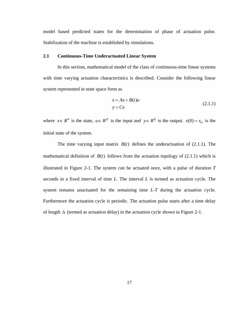
The time varying input matrix ( )B t defines the underactuation of (2.1.1). The
mathematical definition of ( )B t follows from the actuation topology of (2.1.1) which is
illustrated in Figure 2-1. The system can be actuated once, with a pulse of duration T
seconds in a fixed interval of time L. The interval L is termed as actuation cycle. The
system remains unactuated for the remaining time L-T during the actuation cycle.
Furthermore the actuation cycle is periodic. The actuation pulse starts after a time delay
of length Δ (termed as actuation delay) in the actuation cycle shown in Figure 2-1.
Page 31
18
Figure 2-1. Single Actuation Cycle of Period L
The phase (starting point) of the actuation pulse depends upon qr R∈ , which is
the desired reference for stabilization of the output ( )y t . The amplitude of actuation
pulse is fixed in a given actuation cycle, i.e it is zero-order-held. In light of the above
discussion, the input matrix ( )B t is defined as
( )0 otherwiseB kL t kL T
B t+ Δ ≤ ≤ + Δ +⎧
= ⎨⎩
(2.1.2)
where k is a positive integer and ( )n pB × is time invariant matrix. The ( , )A B pair is
assumed to be controllable [45], [76].
2.2 Discrete-Time Equivalent Model
The actuation characteristics of the system (2.1.1) discussed in section 2.1 provide
basis for the development of a discrete-time equivalent model for this system. The
resultant model facilitates discrete-time control law design.
The discrete-time equivalent model is developed for a complete actuation cycle
from t kL= + Δ to t kL L= + Δ + .The equivalent model is developed in two stages. In
Δ
kL ( 1)k L+ T time t
Input u(t)
Page 32
19
the first stage, the time interval [ , ]kL kL T+ Δ + Δ + is considered during which the
system (2.1.1) is actuated with zero-order-held input. In the second stage, the interval
[ , ]kL T kL L+ Δ + + Δ + is considered, for which system (2.1.1) is unactuated.
The state of (2.1.1) at t kL= + Δ is ( )x kL + Δ . The state of this system at
t kL T= + Δ + in terms of ( )x kL + Δ is given by
( )( ) exp( ) ( ) exp ( ) ( ).kL T
kL
x kL T AT x kL A kL T u kL Bdσ σ+Δ+
+Δ
+ Δ + = + Δ + + Δ + − + Δ∫ (2.2.1)
Using change of variables for the integrand, the equation (2.2.1) can be written as
( )
0
1 1
( ) exp( ) ( ) exp ( ) . . ( )
( ) ( )
T
d d
x kL T AT x kL A T d B u kL
A x kL B u kL
σ σ+ Δ + = + Δ + − + Δ
= + Δ + + Δ
∫ (2.2.2)
where 1 exp( )dA AT= and ( )10
exp ( ) .T
dB A T Bdσ σ= −∫ .
Now the interval [ , ]kL T kL L+ Δ + + Δ + is considered. The state of (2.1.1) at
t kL L= + Δ + in terms of ( )x kL T+ Δ + is given by
2
( ) exp( ( )) ( )( )d
x kL L A kL L kL T x kL TA x kL T
+ Δ + = + Δ + − −Δ − + Δ += + Δ +
(2.2.3)
where 2 exp( ( ))dA A L T= − . The complete model from kL + Δ to kL L+ Δ + is obtained
by substituting (2.2.2) in (2.2.3)
( ) ( ) ( )d dx kL L A x kL B u kL+ Δ + = + Δ + + Δ , (2.2.4)
where 2 1d d dA A A= and 2 1d d dB A B= . The equation (2.2.4) is transformed into discrete-
time domain by replacing kL + Δ by m, and kL L+ Δ + by 1m + ,
Page 33
20
[ 1] [ ] [ ]d dx m A x m B u m+ = + . (2.2.5)
The conventional bracket notation is adopted for discrete-time representation. The model
(2.2.5) is the discrete-time equivalent model of (2.1.1) for a single actuation cycle.
2.3 Discrete-time Controller
Stabilization of the system (2.1.1) using a discrete-time controller requires the
controller to determine the magnitude of the actuation pulse. The magnitude of actuation
pulse is determined from a state feedback control law designed on the basis of discrete-
time equivalent model (2.2.5).
The remarkable feature of the discrete-time equivalent model (2.2.5) is that it is
time invariant and fully actuated. Control law design for fully actuated linear time
invariant systems using pole placement is a well known procedure [20]. Consequently the
discrete-time state feedback control law for the stabilization of (2.2.5) is given by
[ ] [ ]u m Kx m Gr= − + . (2.3.1)
where the matrix K is chosen so that the eigenvalues of ( )d dA B K− are inside the unit
circle. The factor G is known as pre-scalar in control system literature and is given by
the following expression ([30], [76])
11
( )d d dG
C A B K I B−= −− −
. (2.3.2)
An important point that should be noted here is that the discrete-time controller
has to determine the phase of actuation pulse ( t kL= + Δ ) as well. The phase of actuation
pulse depends upon the reference for stabilization r and the system state. The discrete-
Page 34
21
time controller decides about the point of actuation during the actuation cycle on the basis
of sampled state [ ]x i , sampled after every T seconds.
Remark 2.1: The discrete-time equivalent model considers a complete actuation cycle of
duration L seconds as a single discrete step, represented by discrete index m, whereas the
sampling time for the discrete-time controller is T seconds represented by discrete index
‘ i ’. The controller sampling rate is usually a fraction of L . Alternately speaking, the
system is two time scale: one scale for the model and the other for the controller.
The controllability (reachability) of ( , )d dA B pair is guaranteed by the following
Lemma
Lemma 2.1
Controllability of ( , )A B pair guarantees controllability of ( , )d dA B pair
Proof
Controllability of ( , )A B pair guarantees that the following controllability
gramian M is of rank n , i.e
2 1[ , , ............ ]nrank B AB A B A B n− = (2.3.3)
The controllability gramian for ( , )d dA B pair is given by
( )
2 1
2 1
0
[ , , ............ ]
exp( ). exp ( ) . [ , , ............ ]
nd d d d d d d d
Tn
d d d
M B A B A B A B
AT A T Bd B A B A B A Bσ σ
−
−
=
= − ×∫ (2.3.4)
Page 35
22
Since exp( )dA AL= , all its powers are full rank because of exponential function being
nonsingular, Similar argument is valid for the term ( )0
exp( ). exp ( )T
AT A T dσ σ−∫ .
Consequently
( ) 2 1
0
( ) exp( ). exp ( ) . [ , , ............T
nd d d drank M rank AT A T Bd B A B A B A B nσ σ −⎛ ⎞= − × =⎜ ⎟⎜ ⎟
⎝ ⎠∫ (2.3.5)
Thus ( , )d dA B is controllable.
2.4 System with Delayed Input
In this section a control law design procedure is presented for the stabilization of
the underactuated system under discussion, with input delay. In the case of input delay,
the dynamics of the system respond to the applied input after certain interval of time. In
recent past, a transformation was presented in [89], termed as linear predictor, that
transforms a discrete-time system with input delay into an equivalent discrete-time
system without input delay. This process facilitates control law design.
The analyses in [89] are for a single time scale discrete-time system, however as
already mentioned, the underactuated systems discussed in this thesis become two time
scale when controlled by a discrete-time controller. Thus modifications have to be done
in the transformation presented in [89] to make it applicable for two time scale systems.
The transformation of [89] is briefly presented here for the convenience of readers.
Page 36
23
Consider the following discrete-time linear system with input delay of N
samples
[ 1] [ ] [ ]x k Ax k Bu k N+ = + − . (2.4.1)
To transform the system into an equivalent model with no input delay, the following
change of variables is performed
1 2
1( 1)
[ ] [ ] [ ] [ 1] .... [ 1]
[ ] [ ]
N
kj k N
j k N
z k x k A Bu k N A Bu k N A Bu k
x k A Bu j
− − −
−− − + +
= −
= + − + − + + + −
= + ∑ (2.4.2)
The dynamics of the transformed variable [ ]z k are represented by
1
( 1)[ 1] [ 1] [ 1]k
j k N
j k Nz k x k A Bu j
−− − + +
= −+ = + + +∑ . (2.4.3)
Upon algebraic manipulations, the following system is achieved
[ 1] [ ] [ ]Nz k Az k A Bu k−+ = + . (2.4.4)
The discrete-time model (2.4.4) has no input delay. Thus the transformation (2.4.2)
converts a discrete-time system with input delays into an equivalent system without any
input delay.
2.4.1 Transformation for Underactuated Linear Systems
Consider that the class of underactuated linear systems under discussion has input
delay of NT seconds. It is assumed that NT L< . The continuous-time model then
becomes
( ) ( ) ( ) ( )( ) ( )
x t Ax t B t u t NTy t Cx t
= + −=
(2.4.5)
Page 37
24
where ( )B t is as defined in (2.1.2). The overall actuation characteristics of the system
(2.4.5) are the same as discussed in section 2.1.
The discrete-time equivalent model for (2.4.5) is developed in two stages, as for
the system without input delay. In the first stage, dynamics of the system for time interval
[ , ]kL kL T+ Δ + Δ + are considered. Following a procedure similar to the one discussed in
section 2.2, it can be shown that the state of the system (2.4.5) at time t kL T= + Δ + in
terms of the state ( )x kL + Δ is given by the following expression
1 1( ) ( ) ( )d dx kL T A x kL B u kL NT+ Δ + = + Δ + + Δ − . (2.4.6)
Representing time kL + Δ by i , kL T+ Δ + by 1i + and switching to conventional
bracket notation for discrete-time representation, (2.4.6) can be written as
1 1[ 1] [ ] [ ]d dx i A x i B u i N+ = + − (2.4.7)
The discrete-time system (2.4.7) can be transformed into an equivalent system without
input delay by the following change of variables
1
( 1)11[ ] [ ] [ ]
ij i N
ddj i N
z i x i A B u j−
− − + +
= −= + ∑ . (2.4.8)
Dynamics of the transformed systems are represented by
1
( 1)1[ 1] [ 1] [ 1]
ij i N
dj i N
z i x i A Bu j−
− − + +
= −+ = + + +∑ . (2.4.9)
The transformed system without input delay is given by
1 1 1[ 1] [ ] [ ]Nd d dz i A z i A B u i−+ = + . (2.4.10)
Page 38
25
The discrete-time model for the transformed system in the interval
[ , ]t kL T kL L∈ +Δ + + Δ + is now developed. Let i M kL L+ = + Δ + , where M LΔ = ,
then,
11[ ] [ 1]M
dz i M A z i−+ = + . (2.4.11)
Since 1AT
dA e= , then 1 ( )1
M A L TdA e− −= .
The complete discrete-time equivalent model without input delay for the
continuous-time system (2.4.5) considering the interval [ , ]t kL kL L∈ +Δ + Δ + as a single
discrete step is
2 1 2 1 1' '
[ 1] [ ] [ ]
[ ] [ ]
Nd d d d d
d d
z m A A z m A A B u m
A z m B u m
−+ = +
= + (2.4.12)
where m i kL= = + Δ , 1m i M kL L+ = + = + Δ + , '2 1d d dA A A= and '
2 1 1N
d d d dB A A B−= .
2.4.2 Control law Design
The continuous-time underactuated system with delayed input (2.4.5) is stabilized
by a discrete-time control law designed on the basis of discrete-time fully actuated, time
invariant equivalent model without input delay (2.4.12). The matrix K is chosen so that
the eigenvalues of ' 'd dA B K− are inside the unit circle. The feedback control input is
calculated in terms of the original coordinates as
( )1 1
[ ] [ ]
[ ] [ ]Nd d
u m Kz m Gr
K x i A B u i N Gr−
= − +
= − − − + (2.4.13)
where the pre-scalar G is obtained using (2.3.2). Equation (2.4.13) implies
( )1 1[ ] [ ] [ 1]Nd du i N K x i N A B u i N Gr−− = − − − − − + . (2.4.14)
Page 39
26
Since [ 1] 0u i N− − = ,
[ ] [ ]u i N Kx i N Gr− = − − + . (2.4.15)
2.5 Example: The Underactuated Drill Machine
Multi-axis drilling is a well known industrial application. Drilling on curved
surfaces requires precise orientation control of the drill bit so that the axis of the bit is
preferably normal to the surface at the point of drilling. This orientation adjustment
requires two independent actuators for pitch and yaw that make the drill machine quite a
complex system. In a special application of drilling the soft materials, negligible lateral
resistance is experienced by the drill bit. Consequently, once the bit is oriented in the
desired direction, negligible change in control effort is experienced. Therefore, for
precise drilling, only orientation control instead of a complete compliance control of the
bit is required.
A special drill machine whose orientation control mechanism is specifically
designed for drilling soft materials only is considered here. The remarkable feature of the
actuation mechanism is that the orientation control of the drill bit is achieved using a
single pair of electromagnetic poles. The magnetic field of these poles interacts with the
field of the rotor which is a permanent magnet to produce a torque that changes the
orientation of the drill bit. The electromagnetic poles are excited for a short duration at
specific roll phase to orient the bit in the desired direction. The special actuation
mechanism reduces the number of actuators to one as opposed to the two actuators
generally required for the control of two degrees of freedom; hence a simpler system is
achieved.
Page 40
27
2.5.1 Construction and Operation
The underactuated drill machine used for multi-axis drilling of soft nonmagnetic
materials has customized construction. This special construction enables the use of a
single pair of electromagnetic poles to control two degrees of freedom, i.e pitch and yaw,
of the bit. For clarity of presentation, construction of the orientation control mechanism is
explained only.
The rotor of the machine is a ring shaped permanent magnet as shown in Figure
2-2. The rotor is connected to the base of the machine by a universal joint which provides
the roll, pitch and yaw freedoms. It may be noted here that the base of the machine may
be mounted on a manipulator for enhancement of the workspace as desired. The stator of
the machine has a single coil wound over it as shown in Figure 2-2. Excitation of this coil
produces the orientation control field which is always aligned with the z axis of the fixed
frame of reference (x,y,z). Interaction of the orientation control magnetic field with the
field of the rotor permanent magnet results in torque that changes the orientation of the
bit.
It is assumed that the drill bit is rotating about the 'z axis of the rotating frame of
reference ( ' ' ', ,x y z ) at constant rpm ω . In Figure 2-2, only 'z axis is shown for simplicity
which is aligned with the z axis. This is also the reference position for measurement of
the angular displacement of the bit about x and y axes. The roll actuation and speed
stabilization are handled separately. However the roll actuation mechanism can also be
integrated on the same stator.
Page 41
28
Figure 2-2. Construction of the Underactuated Drill Machine
2.5.2 Actuation Mechanism
Consider that the bit is spinning about 'z axis at constant rpm ω thus the
dynamical behavior of the bit is that of spinning gyroscope. To explain the actuation
mechanism suppose that the bit is at the reference position ( z and 'z axes aligned) and it
is to be rotated by 1θ and 2θ radians about x and y axes of the fixed reference frame
respectively. P̂ is the unit vector of the projection of the final position of the bit in the xy
plane as indicated in Figure 2-3. To achieve the desired orientation, the stator
electromagnet is energized when the field of the permanent rotor magnet is perpendicular
to the vector P̂ as shown in Figure 2-3. Similar poles experience repulsive force while
opposite poles experience attractive force in the z axis direction. This results in torque τ
aligned to the vector P̂ . Since the bit is spinning about 'z axis, it rotates about the axis
perpendicular to the axis of spin and applied torque according to law of conservation of
z
x
Stator Winding
Permanent Rotor Magnet
y
'z
N
S
Page 42
29
angular momentum, consequently it moves towards vector P̂ , a phenomena known as
precession in gyroscopes. The magnitude of τ depends upon the magnitude of applied
current in the stator coil. The torque vector can be resolved into two rectangular
components xτ and yτ .
The important aspects of the actuation mechanism are summarized in following
three points
1. A single actuation signal (current through the stator coil) controls two degrees of
freedom: the pitch and yaw of the bit, thus explaining the underactuation of the
drill machine.
2. The actuation pulse is applied for a short duration when the field of the permanent
rotor magnet and the unit vector of the projection of the desired position of the bit
are considered approximately perpendicular. This duration is usually a fraction of
the time period for a complete rotation of the drill bit.
3. The actuation pulse can be applied once in a complete revolution of the bit. The
system remains unactuated during the remaining time of a revolution.
Page 43
30
Figure 2-3. Position of Actuation
2.5.3 Continuous-time Model
As it has been mentioned in section 2.5.2 that the drill bit can be treated as a
spinning gyroscope, the dynamical model of a gyroscope is used here for representing the
bit. The simplified dynamical model of a spinning gyroscope is given by the following
equations
x x y i x
y y x i y
J b H K
J b H K
θ θ θ τ
θ θ θ τ
+ + =
+ − = (2.5.1)
where xθ and yθ represent the angular positions of the bit in radians about x and y
axes respectively, xτ and yτ are the torques applied about x and y axes respectively, J is
the moment of inertia, b is the coefficient of friction, iK is the torque constant. H is
y
x
P̂ N
S
Rotor Magnetic field spinning at ω rpm
Page 44
31
angular momentum defined by the expression ( )zH J J ω= − , (where ω is the spin
frequency of the bit about 'z axis) and zJ is the moment of inertia of the bit about 'z
axis.
The model (2.5.1) is represented in state space form by defining xθ and yθ as
states 1x and 3x respectively. The derivates of angular positions i.e xθ and yθ are
represented by states 2x and 4x respectively and the applied torques xτ and yτ are
considered as inputs 1u and 2u respectively. The state space representation of (2.5.1) is
given by
1 2
2 2 4 1
3 4
4 3 2 2
i
i
x xKb Hx x x u
J J Jx x
Kb Hx x x uJ J J
=
= − − +
=
= − + +
(2.5.2)
The states 1x and 3x are considered as output y of the system since these states have to
be stabilized at desired reference r . The model (2.5.2) can be written in the convenient
matrix form as
x Ax Buy Cx= +=
(2.5.3)
Page 45
32
where
0 00 1 0 0/ 00 / 0 /
,0 00 0 0 10 /0 / 0 /
1 0 0 00 0 1 0
i
i
K Jb J H JA B
K JH J b J
C
⎡ ⎤⎡ ⎤⎢ ⎥⎢ ⎥− − ⎢ ⎥⎢ ⎥= =⎢ ⎥⎢ ⎥⎢ ⎥⎢ ⎥−⎣ ⎦ ⎣ ⎦
⎡ ⎤= ⎢ ⎥⎣ ⎦
(2.5.4)
The drill bit can be actuated for a short duration when the desired projection
vector and permanent magnet are approximately perpendicular. The bit is unactuated
otherwise during the roll. The underactuation of the bit is introduced in the model (2.5.3)
as
( )x Ax B t u
y Cx= +=
(2.5.5)
where ( )B t is as defined in (2.1.2) with B given in (2.5.4), L is equal to the time period
of roll and T is the duration during which the desired projection vector and permanent
magnet are considered approximately perpendicular.
2.5.4 Discrete-time Controller
The control objective is the stabilization of the drill bit at the desired reference
using a discrete-time controller. For this purpose, it is assumed that feedback of all the
system states is available to the controller. Moreover, feedback of the position of the rotor
is also available. The discrete-time controller has the following two objectives
A: Determination of the magnitude of control input according to a state feedback
control law.
Page 46
33
B: Determination of the point of actuation during the roll of the bit. The point of
actuation depends upon the angular position of the permanent magnet.
The state feedback control law is designed on the basis of discrete-time equivalent
model of the drill bit developed according to the procedure presented in section 2.2 using
pole placement procedure. The matrix K is chosen so that the eigenvalues of
( )d dA B K− are inside the unit circle. The control input is given by
[ ] [ ]u m Kx m Gr= − + . (2.5.6)
The second task of the discrete-time controller is the determination of the point of
actuation t kL= + Δ during roll of the bit. To determine the phase of actuation pulse it is
assumed that state feedback [ ]x i and angular position feedback of the permanent rotor
magnet [ ]iα is available to the controller after every T seconds which is indicated by
discrete index i .
It should be noted here that the feedback control input (2.5.6) gives the required
torque vector whose phase will always by perpendicular to the desired projection unit
vector P̂ described in section 2.5.2. In order to determine the centre of actuation pulse,
the controller computes a feedback control input [ ]u i after every T seconds on the basis
of the sampled state feedback [ ]x i . The center of actuation pulse is at the discrete index i
at which the following condition is satisfied
1 2
1
[ ][ ] tan[ ] 2
u iiu i
πα − ⎛ ⎞= +⎜ ⎟
⎝ ⎠, (2.5.7)
where [ ]pu i is the thp component of the 2 1× vector [ ]Kx i Nr− + .
Page 47
34
The condition (2.5.7) marks the centre of actuation pulse for the system as shown
in Figure 2-1. The actuation of the system has to start / 2T seconds prior to the point in
time when this condition is satisfied. This makes the system actuation non-causal. To
overcome this non-causality, model prediction based determination of point of actuation
is suggested in which case the system states at the next discrete step are estimated. Based
on these estimates a decision is taken whether or not the next discrete index would be the
centre of actuation pulse. In case the next sample marks the centre of actuation pulse,
actuation starts / 2T seconds after the current sample.
The states of the system at the next discrete step can be estimated using the
following expression
1 1ˆ[ 1] [ ] [ ]d dx i A x i B u i+ = + . (2.5.8)
The estimated state ˆ[ 1]x i + is then used by the controller in deciding about actuation or
otherwise at 2Tt iT= + . Mathematically,
( )1 2
1
ˆ [ 1]ˆ[ 1] [ ] tan [ / 2, ( 1) / 2]ˆ [ 1] 2
0 otherwise
u iKx i Gr if i t iT T i T Tu t u i
πα −⎧ ⎛ ⎞+− + + = + ∀ ∈ + + +⎪ ⎜ ⎟= +⎨ ⎝ ⎠⎪⎩
(2.5.9)
where ˆ [ 1]pu i + is the thp component of the 2 1× vector ˆ[ 1]Kx i Gr− + + .
2.5.5 Simulations
Simulation of the drill machine controlled by discrete-time algorithm discussed in
section 2.2 is presented in this section. A case of drill machine having delayed input is
Page 48
35
also considered for simulation [62]. The input delay is assumed to be of a single sampling
interval. The control law is designed using the procedure presented in section 2.4.
The various parameters of the drill machine used for simulation are 24 Kg-m ,J =
25 Kg-m ,zJ = 400 rad/sec,ω π= 1iK = and =100b . The drill machine is assumed to be
at rest initially and the desired reference for stabilization is [0.4,0.3]Tr = . The time
duration of a single revolution about 'z -axis is 0.05L s= . The sampling time and
duration of actuation is / 16T L= . The matrices dA and dB of the discrete-time
equivalent model as described in section 2.2 are
4
1 0.0036 0 -0.0014 0.0028 -0.00100 0.4289 0 -0.4289 0.3486 -0.3318
, 100 0.0014 1 0.0036 0.0010 0.00280 0.4289 0 0.4289 0.3318 0.3486
d dA B −
⎡ ⎤ ⎡ ⎤⎢ ⎥ ⎢ ⎥⎢ ⎥ ⎢ ⎥= = ×⎢ ⎥ ⎢ ⎥⎢ ⎥ ⎢ ⎥⎣ ⎦ ⎣ ⎦
(2.5.10)
The matrix K is chosen for the control law (2.3.1) so that the eigenvalues of
d dA B K− are inside the unit circle. The results of simulation are presented in Figure 2-4,
which shows that the continuous-time system is stabilized at the desired reference.
Stabilization of the drill bit at the desired reference with delayed input of a single
sample is shown in Figure 2-5 . In case of delayed system 'd dA A= and
' 4
0.0026 -0.00090.3760 -0.3243
100.0009 0.00260.3243 0.3760
dB −
⎡ ⎤⎢ ⎥⎢ ⎥= ×⎢ ⎥⎢ ⎥⎣ ⎦
. (2.5.11)
The matrix K is chosen for the control law (2.4.13) so that the eigenvalues of ' 'd dA B K−
are inside the unit circle.
Page 49
36
Figure 2-4. Stabilization of the Drill Bit without Input Delay
Page 50
37
Figure 2-5. Stabilization of the Drill Bit with Input Delay of a Single Sample
Page 51
38
2.6 Summary
A discrete-time control algorithm is discussed for sampled-data control of a class
of underactuated linear systems. The said class of systems has time varying actuation
characteristics. The system can be actuated with a short duration pulse whose period is a
fraction of the complete actuation cycle. To design the control law, a time invariant, fully
actuated discrete-time equivalent model of the continuous-time system is developed.
Systems having actuation delays are also considered in the development of the control
algorithm. The application of the algorithm is illustrated by the orientation control of an
underactuated drill machine whose two degrees of freedom can be controlled by a single
actuator. Simulation of the closed loop system shows that the drill machine is stabilized
at the desired reference.
Page 52
39
CHAPTER 3
DISCRETIZATION ERROR BOUNDS FOR NONLINEAR SYSTEMS
In this chapter discretization error bounds are determined for locally Lipschitz
nonlinear systems discretized using the Euler method. Characteristics of the discretization
error effect the performance of the control law designed on the basis of the discretized
system model. The need for new development arises from the fact that the discretization
error bounds derived for locally Lipschitz nonlinear systems in literature are quite
abstract and loose.
The discussion starts with the revisit of the Lipschitz condition followed by the
review of local existence and uniqueness theorem for locally Lipschitz nonlinear systems.
This theorem guarantees that a unique solution exists for a specific time interval. It is
shown that the discretization error remains bounded for a single sampling interval with
sampling time less than the time interval of guaranteed existence of solution. Afterwards,
discretization error bounds are established for more than one sampling interval.
The analyses are illustrated by two examples. In the first example a locally
Lipschitz nonlinear system with finite escape time is considered. For a specified sampling
time, discretization error bound is calculated and it is shown that the actual error remains
within calculated bounds. The alternate application of the error bound analysis is the
determination of variable step-size for specified error bounds in numerical solvers. In the
second example a nonlinear system which is not continuously differentiable, is
considered. In this case also, the actual discretization error remains within bounds.
Page 53
40
3.1 Single-Step Input Discretization Error Bound
Consider the following nonlinear system
( , ), (0) ox f x u x x= = , (3.1.1)
where nx R∈ is the state and mu R∈ is the input, which is assumed to be bounded.
(0) ox x= is the initial condition of the system.
3.1.1 Assumption 1
The function ( , )f x u is assumed to be locally Lipschitz in x and u over balls xB
and uB respectively. Mathematically,
( ) ( ) 1, , , xf x u f y u L x y x y B− ≤ − ∀ ∈ , (3.1.2)
where
{ }x o xB x x x r= − ≤ , (3.1.3)
and
( ) ( ) 2, , , uf x u f x v L u v u v B− ≤ − ∀ ∈ , (3.1.4)
where
{ }u uB u u r= ≤ . (3.1.5)
Remark 3.1: Definition (3.1.5) also specifies the bound on input ( )u t . It should be noted
here that the ball defined in (3.1.5) is independent of ou which is the initial value of the
input. The reason is that the signal ( )u t is not evolving as a result of solution of a
differential equation as opposed to ( )x t . Thus ( )u t can be assumed independent of ou .
Page 54
41
Remark 3.2: The notation . indicates vector norm. The choice of norm in the analyses
is not important and the results hold for any p-norm.
Theorem 3.1 (Local Existence and Uniqueness) [49]
Under Assumption 1, there exists 0δ > such that the state equation (3.1.1) has a
unique solution over the time interval [ ]0,δ . The conditions satisfied by δ are as
follows [49].
1 1 1
min ,x
x
rL r h L
ρδ⎧ ⎫
≤ ⎨ ⎬+⎩ ⎭, (3.1.6)
where
1 max ( , )ou Bu
h f x u∈
= , (3.1.7)
and ρ is a positive number satisfying 1ρ < . It may also be noted that under the stated
conditions, the state ( )x t remains inside the ball of radius xr for all [0, ]t δ∈ ,[49].
3.1.2 System with Zero-Order-Held Input
Consider an approximation of the system (3.1.1) when the input is held constant
for time [ ]0,t T∈ , where T δ≤ . This new system can be expressed as follows
( , ), (0)(0)
o o
o
z f z u z xu u
= ==
, (3.1.8)
where z is the state and ou is the held input. Existence and uniqueness of (3.1.8) is
guaranteed by Theorem 2.1, where (3.1.7) simplifies into
Page 55
42
( , )o oh f x u= . (3.1.9)
The difference between the states of (3.1.1) and (3.1.8) is defined as input
discretization error. Mathematically,
( ) ( ) ( ), [0, ]ue t x t z t t T= − ∈ , (3.1.10)
which gives
( ) ( , ) ( , ), ( ) 0.
( )u o o
o o
e t f x u f z u e tu t u
= − ==
(3.1.11)
Theorem 3.2
Under the stated conditions of Theorem 3.1, the norm of the input discretization
error (3.1.10) at time *T δ≤ satisfies the following inequality
' '1 2( ) 2 2u ue T TL r TL r≤ + , (3.1.12)
where
' ' 'max( , )x zr r r= , (3.1.13)
'[0, ]
max ( )x oT
r x xτ
τ∈
= − , (3.1.14)
'[0, ]
max ( ) (0)zT
r z zτ
τ∈
= − , (3.1.15)
'[0, ]
max ( )uT
r uτ
τ∈
= , (3.1.16)
and
*1min( , )δ δ δ= , (3.1.17)
Page 56
43
with 11
1L
δ < .
Proof
Integrating (3.1.11) over [ ]0,T
( ) ( ) [ ]0
( ) ( ), ( ) ( ), 0,t
u oe t f x u f z u d t Tτ τ τ τ⎡ ⎤= − ∀ ∈⎣ ⎦∫ . (3.1.18)
Taking norm of both sides of (3.1.18), and using Gram-Schmidt inequality
( ) ( ) [ ]
( ) ( ) [ ]
0
0
( ) ( ), ( ) ( ), 0,
( ), ( ) ( ), 0,
t
u o
t
o
e t f x u f z u d t T
f x u f z u d t T
τ τ τ τ
τ τ τ τ
= − ∀ ∈
≤ − ∀ ∈
∫
∫ (3.1.19)
Adding and subtracting ( ( ), ( ))f z uτ τ inside the integrand and subsequently using the
triangle inequality of vector norms ( )a b a b+ ≤ + results in
( ) ( )
( ) ( )
0
0
( ) ( ), ( ) ( ( ), ( )) ( ( ), ( )) ( ),
( ), ( ) ( ( ), ( )) ( ( ), ( )) ( ),
t
u o
t
o
e t f x u f z u f z u f z u d
f x u f z u f z u f z u d
τ τ τ τ τ τ τ τ
τ τ τ τ τ τ τ τ
≤ − + −
≤ − + −
∫
∫ (3.1.20)
Applying Lipschitz conditions
1 20 0
( ) ( ) ( ) ( )t t
u oe t L x z d L u u dτ τ τ τ τ≤ − + −∫ ∫ . (3.1.21)
Adding and subtracting ox inside the vector norm of the first integrand of (3.1.21)
Page 57
44
1 2
0 0
1 20 0
( ) ( ) ( ) ( )
( ( ) ) ( ( ) ) ( )
t t
u o o o
t t
o o o
e t L x x z x d L u u d
L x x z x d L u u d
τ τ τ τ τ
τ τ τ τ τ
≤ ⎡ − − + ⎤ + ⎡ + ⎤⎣ ⎦ ⎣ ⎦
≤ ⎡ − − − ⎤ + ⎡ + ⎤⎣ ⎦ ⎣ ⎦
∫ ∫
∫ ∫ (3.1.22)
Using triangular inequality of vector norms again gives
1 20 0
( ) ( ) ( ) ( )t t
u o o oe t L x x z x d L u u dτ τ τ τ τ≤ ⎡ − + − ⎤ + ⎡ + ⎤⎣ ⎦ ⎣ ⎦∫ ∫ . (3.1.23)
Using definitions of ' ' ', and x z ur r r as given in (3.1.14)-(3.1.16), the inequality (3.1.19)
transforms into
1 1 2 20 0 0 0' ' '
1 1 2
( ) ( ) ( ) ( )
2
t t t t
u o o o
x z u
e t L x x d L z x d L u d L u d
L r t L r t L r t
τ τ τ τ τ τ τ≤ − + − + +
≤ + +
∫ ∫ ∫ ∫ (3.1.24)
Using definition of 'r given in (3.1.13)
' '1 2( ) 2 2u ue t L r t L r t≤ + . (3.1.25)
Thus the norm of a single-step input discretization error satisfies the following inequality
' '1 2( ) 2 2u ue T TL r TL r≤ + . (3.1.26)
Remark 3.3: The existence and uniqueness of solutions of (3.1.1) and (3.1.8) (as
guaranteed by Theorem 2.1), ensures validity of (3.1.14) and (3.1.15) which are bounds
for the trajectories of nonlinear systems (3.1.1) and (3.1.8) respectively for time interval
[0, ]T . Bounds for (3.1.14) and (3.1.15) are determined as follows
Page 58
45
3.1.3 Bound for 'xr
Integrating (3.1.1) over [0, ]T
( ) ( )0
( ), ( ) [0, ]t
ox t x f x u d t Tτ τ τ= + ∀ ∈∫ . (3.1.27)
Rearranging (3.1.27)
( ) ( )0
( ), ( ) [0, ]t
ox t x f x u d t Tτ τ τ− = ∀ ∈∫ . (3.1.28)
Taking norm of both sides and using Gram-Schmidt inequality
( ) ( )0
( ), (t
ox t x f x u dτ τ τ− ≤ ∫ . (3.1.29)
Adding and subtracting ( ), ( )of x u τ
( ) ( ) ( ) ( )
( ) ( ) ( )
0
0
( ), ( ) , ( ) , ( )
( ), ( ) , ( ) , ( )
t
o o o
t
o o
x t x f x u f x u f x u d
f x u f x u f x u d
τ τ τ τ τ
τ τ τ τ τ
⎡ ⎤− ≤ − +⎣ ⎦
⎡ ⎤≤ − +⎣ ⎦
∫
∫ (3.1.30)
Equations (3.1.2) and (3.1.7) transforms inequality (3.1.30) into
( ) 1 10
[ ( ) ] [0, ]t
o ox t x L x x h d t Tτ τ− ≤ − + ∀ ∈∫ . (3.1.31)
Since the inequality (3.1.31) holds for all [0, ]t T∈ , then it holds for the time instant
where the maximum value ( ) ox t x− occurs. Thus the following expression can be
written
( )' '1 1x xr L r h T≤ + . (3.1.32)
Page 59
46
Rearrangement of (3.1.32) results in
' 1
1( ) [0, ]
1o xh Tx t x r t T
L T− ≤ ≤ ∈
−. (3.1.33)
The condition that 11
1L
δ < ensures that (3.1.33) is positive semi definite.
3.1.4 Bound for 'zr
Bound for equation (3.1.15) can be obtained in a manner similar to which the
bound for 'xr is obtained. Integrating (3.1.8)
( ) ( )00
(0) ( ), [0, ]t
z t z f z u d t Tτ τ= + ∀ ∈∫ . (3.1.34)
Rearranging and taking norm of both sides leads to
( ) ( )0
( ), [0, ]t
o oz t x f z u d t Tτ τ− ≤ ∀ ∈∫ . (3.1.35)
Adding and subtracting ( ),o of x u inside the integrand of (3.1.35)
( ) ( ) ( ) ( )0
( ), , ,t
o o o o o oz t x f z u f x u f x u dτ τ⎡ ⎤− ≤ − +⎣ ⎦∫ . (3.1.36)
Using (3.1.2) and (3.1.9) in (3.1.36) gives
( ) 10
[ ( ) ] [0, ]t
o oz t x L z x h d t Tτ τ− ≤ − + ∀ ∈∫ . (3.1.37)
As in case of (3.1.31), the inequality (3.1.37) holds for all [0, ]t T∈ , therefore
( )' '1z zr L r h T≤ + . (3.1.38)
Page 60
47
Rearrangement of (3.1.38) gives the following expression
'
1( ) . [0, ]
1o zhTz t x r t TL T
− ≤ ≤ ∈−
. (3.1.39)
3.2 Single-Step Model Discretization Error Bound
3.2.1 Discretized System Model
Nonlinear systems are discretized by approximating the derivative by forward
difference [54] i.e.
[ 1] [ ]( ) x k x kx kTT
+ −≈ , (3.2.1)
where T is the sampling time and [ ] ( )x k x kT= is the sampled state at time t kT= . The
conventional bracket notation and discrete indexing is used for discrete entities
throughout the Thesis. Input to the system is discretized by holding it constant during the
sampling interval, (zero-order-hold [33]). Since the same has already been treated in
Section 3.1.2, only the Euler method needs to be applied here to get a discrete system as
follows
[ 1] [ ] ( [ ], [ ]) [0]a a a a ox k x k Tf x k u k x x+ = + = . (3.2.2)
Remark 3.4: Throughout this thesis, the subscript ‘a’ with state x indicates that [ ]ax k is
an approximation of the state of a system at time t kT= .
System (3.2.2) can be considered as an approximation of (3.1.8) which in turn is
itself an approximation of (3.1.1). Alternately speaking, discretization is a two-step
procedure.
Page 61
48
The error due to the forward difference approximation is defined as follows
[ ] ( ) [ ] [0] 0d a de k z kT x k e= − = . (3.2.3)
It may be noted that [ ]de k can only be defined in the discrete-time domain.
3.2.2 Single-Step Model Discretization Error
As a first step, the difference between the state of the nonlinear system (3.1.8) at
time t T= that is ( )z T , and the state [1]ax of the approximate system (3.2.2) is
considered, when (0) [0]a oz x x= = . The input ( ) ou t u= remains constant in the interval
[0, ]T . Mathematically the single-step model discretization error is defined as
[1] ( ) [1]d ae z T x= − . (3.2.4)
In this section, it shown that the single-step model discretization error (3.2.4) is
bounded. The following theorem summarizes the results.
Theorem.3.3
Under the stated conditions of Theorem 3.1, there exists a sampling time *T δ≤
such that the norm of the discretization error satisfies the following inequality
2
1
1[1]
1dT L he
L T≤
−, (3.2.5)
where 1L , h and *δ are defined in (3.1.2), (3.1.9) and (3.1.17) respectively.
Page 62
49
Proof
Taking *T δ≤ ensures that the system remains inside the ball of radius xr as
defined in (3.1.3). The state of the nonlinear system with zero-order-held input at time T
is obtained by integrating (3.1.8) over [ ]0,T
( ) ( )00
(0) ( ),T
z T z f z u dτ τ= + ∫ , (3.2.6)
The discrete-time approximation using the Euler method at time T is given by the
following equation
[1] ( , )a o o ox x Tf x u= + . (3.2.7)
From (3.2.4), (3.2.6) and (3.2.7), the following expression is obtained
( )0
[1] ( ), ( , )T
d o o oe f z u d Tf x uτ τ= −∫ . (3.2.8)
Taking norms of both sides and rearranging
( )0
[1] ( ), ( , )T
d o o oe f z u f x u dτ τ≤ −∫ . (3.2.9)
Expressions (3.1.2) and (3.1.3) result in
10
[1] ( )T
d oe L z x dτ τ≤ −∫ . (3.2.10)
Since
'( ) [0, ]o zz t x r t T− ≤ ∀ ∈ , (3.2.11)
the inequality (3.2.10) can be written as
Page 63
50
'1[1]d ze TL r≤ . (3.2.12)
Using the bound on 'zr determined in section 3.1.4 and given by inequality (3.1.39), the
inequality (3.2.12) can be alternatively written as
2
1
1[1]
1dT L he
L T≤
−. (3.2.13)
3.2.3 Total Single-Step Discretization Error
The total discretization error can be defined as
[ ] [ ][ ] ( ) [ ]
( ) ( ) ( ) [ ]( ) [ ]
u d
a
a
e k e kT e kx kT z kT z kT x k
x kT x k
= +
= − + −
= −
(3.2.14)
The norm of total single-step discretization error is defined as
[1] [ ] [1]u de e T e= + . (3.2.15)
The bound on (3.2.15) is obtained by replacing 'zr by r′ in (3.2.12) and using it along
with (3.1.26) in (3.2.15)
( )' '1 2[1] 3 2 ue L r L r T≤ + . (3.2.16)
3.3 Multi-Step Input Discretization Error Bound
In the previous two sections, bounds were determined on the norm of
discretization error for a single sampling interval T which is shown in (3.2.16). At this
point, the idea of discretization is extended beyond a single sampling interval, and
discretization process carried out for a number of time samples is considered. In this case,
Page 64
51
it is quite natural to imagine that as the number of steps increase, the corresponding
discretization error increases accordingly.
As for the case of a single-step discretization error, the multi-step input
discretization error is investigated first, which is the difference between the state of
nonlinear plant (3.1.1) and its approximation with zero-order-held input for sampling
interval T (3.1.8), after N sampling intervals. Mathematically the multi-step input
discretization error is defined as
( ) ( ) ( )ue NT x NT z NT= − . (3.3.1)
Bound on multi-step input discretization error is established by the following theorem.
Theorem 3.3
Under the stated conditions of Theorem 3.1, the norm of input discretization error
after N sampling intervals ( *NT δ≤ ) satisfies the following inequality
'' ''1 2 1( ) 2 2 (1 ) (( 1) )u u ue NT TL r TL r TL e N T≤ + + + − , (3.3.2)
where
'' '' ''max[ , ]x zr r r= ,
''[ ,( 1) ]
max ( ) ( ) [0, 1]xkT k T
r x x kT k Nτ
τ∈ +
= − ∀ ∈ − ,
''[ ,( 1) ]
max ( ) ( ) [0, 1]zkT k T
r z z kT k Nτ
τ∈ +
= − ∀ ∈ − ,
''[0, ]max ( ) .u
NTr u
ττ
∈=
Moreover, the inequality (3.3.2) can be written as
Page 65
52
( )1 '' ''1 2
1
1( ) 2 2NTL
u uee NT L r L r
L⎡ ⎤−
≤ +⎢ ⎥⎢ ⎥⎣ ⎦
. (3.3.3)
Proof
The discretization error at time ( 1)t k T= + with reference to state ( )x kT of the
nonlinear system (3.1.1) and ( )z kT of the approximate nonlinear system (with zero-
order-held input for the sampling interval) (3.1.8) is explored. The index k is any positive
integer and belongs to the interval [0, 1]N − . The state x of the nonlinear system (3.1.1)
in the interval [ , ( 1) ]t kT k T∈ + is given by
( ) ( )( ) ( ), ( ) [ , ( 1) ]t
kT
x t x kT f x u d t kT k Tτ τ τ= + ∀ ∈ +∫ . (3.3.4)
The state z of the approximate nonlinear system with zero-order-held input in the
interval [ , ( 1) ]t kT k T∈ + is given by
( ) ( )( ) ( ), ( ) [ , ( 1) ]t
kT
z t z kT f z u kT d t kT k Tτ τ= + ∀ ∈ +∫ . (3.3.5)
The input discretization error in the interval [ , ( 1) ]t kT k T∈ + can be written as
( ) ( )( ) ( ) ( ) ( ), ( ) ( ), ( ) [ , ( 1) ]t t
ukT kT
e t x kT z kT f x u d f z u kT d t kT k Tτ τ τ τ τ= − + − ∀ ∈ +∫ ∫ (3.3.6)
Using definition of ( )ue kT equation (3.3.6) becomes
( ) ( )( ) ( ) ( ), ( ) ( ), ( ) [ , ( 1) ]t
u ukT
e t e kT f x u f z u kT d t kT k Tτ τ τ τ= + − ∀ ∈ +⎡ ⎤⎣ ⎦∫ (3.3.7)
Adding and subtracting ( )( ), ( )f z uτ τ gives
Page 66
53
( ) ( ) ( ) ( )( ) ( ) ( ), ( ) ( ), ( ) ( ), ( ) ( ), ( )
[ , ( 1) ]
t
u ukT
e t e kT f x u f z u f z u f z u kT d
t kT k T
τ τ τ τ τ τ τ τ= + − + −⎡ ⎤⎣ ⎦
∀ ∈ +
∫
(3.3.8)
Taking norm of both sides and applying Lipschitz conditions results in
1 2( ) ( ) ( ) ( ) ( ) ( ) [ , ( 1) ]t t
u ukT kT
e t e kT L x z d L u u kT d t kT k Tτ τ τ τ τ≤ + − + − ∀ ∈ +∫ ∫ (3.3.9)
Now adding and subtracting ( )x kT and ( )z kT in the second term on the right hand side
of (3.3.9)
1
2 2
( ) ( ) ( ) ( ) ( ) ( ) ( ) ( )
( ) ( ) [ , ( 1) ]
t
u ukTt t
kT kT
e t e kT L x x kT x kT z z kT z kT d
L u d L u kT d t kT k T
τ τ τ
τ τ τ
≤ + + − − + −
+ + ∀ ∈ +
∫
∫ ∫(3.3.10)
Further algebraic manipulation and using definition of ''ur leads to
''1 2
''1 1 1 2
( ) ( ) ( ) ( ) ( ) ( ) ( ) ( ) 2
( ) ( ) ( ) ( ) ( ) ( ) ( ) 2
[ , 2 ]
t
u u ukTt t t
u uT T T
e t e kT L x x kT x kT z kT z z kT d TL r d
e kT L x x kT d L x kT z kT d L z z kT d TL r
t T T
τ τ τ τ
τ τ τ τ τ
≤ + − + − − + +
≤ + − + − + − +
∀ ∈
∫
∫ ∫ ∫
(3.3.11)
Using definition of ( )ue kT , '' '' '', , andx zr r r , transforms (3.3.11) into
Page 67
54
'' '' ''
1 1 1 2'' ''
1 2 1
(( 1) ) ( ) 2
2 2 (1 ) ( )u x z u u
u u
e k T TL r TL r TL e kT TL r
TL r TL r TL e kT
+ ≤ + + +
≤ + + + (3.3.12)
The inequality (3.3.12) for the thN sampling intervals is written as
'' ''1 2 1( ) 2 2 (1 ) (( 1) ) .u u ue NT TL r TL r TL e N T≤ + + + − (3.3.13)
The bound (3.3.13) shows that multi-step input discretization error is a function of
sampling time, Lipschitz constants 1L , 2L and input discretization error at the previous
stage.
Recursive application of (3.3.13) results in ([11])
{ }( )1 '' ''1 1 1 2( ) 1 (1 ) ...... (1 ) 2 2N
d ue NT TL TL TL r TL r−≤ + + + + + + . (3.3.14)
The sum of geometric series (3.3.14) can be written as
( )
( )
'' ''11 2
1
'' ''11 2
1
(1 ) 1( ) 2 21 1
(1 ) 1 2 2
N
u u
N
u
TLe NT TL r TL rTL
TL L r L rL
⎡ ⎤+ −≤ +⎢ ⎥
+ −⎢ ⎥⎣ ⎦⎡ ⎤+ −
≤ +⎢ ⎥⎢ ⎥⎣ ⎦
(3.3.15)
Inequality (3.3.15) can be further simplified using Lemma 1 presented in Chapter 6 of
[11] as
( )1 '' ''1 2
1
1( ) 2 2NTL
u uee NT L r L r
L⎡ ⎤−
≤ +⎢ ⎥⎢ ⎥⎣ ⎦
. (3.3.16)
Remark 3.5: The existence of '' ''andx zr r is guaranteed from the fact that a unique
solution of (3.1.1) and (3.1.8) exists for *NT δ≤ . The bounds for '' ''andx zr r can be
derived in a manner analogous to the one used for the derivation of bounds for ' 'andx zr r .
Page 68
55
3.3.1 Bound for ''xr
Using (3.3.4) for arbitrary k which belongs to the interval [0, 1]N −
( ) ( )( ) ( ), ( ) [ , ( 1) ]t
kT
x t x kT f x u d t kT k Tτ τ τ− = ∈ +∫ . (3.3.17)
Taking norm and applying Gram Schmidt inequality
( ) ( )( ) ( ), ( ) [ , ( 1) ]t
kT
x t x kT f x u d t kT k Tτ τ τ− ≤ ∈ +∫ . (3.3.18)
Adding and subtracting ( )( ), ( )f x kT u τ
( ) ( ) ( ) ( )
( ) ( ) ( )
0
0
( ) ( ), ( ) ( ), ( ) ( ), ( )
( ), ( ) ( ), ( ) ( ), ( )
t
t
x t x kT f x u f x kT u f x kT u d
f x u f x kT u f x kT u d
τ τ τ τ τ
τ τ τ τ τ
⎡ ⎤− ≤ − +⎣ ⎦
⎡ ⎤≤ − +⎣ ⎦
∫
∫(3.3.19)
Applying Lipschitz condition
( ) 10
( ) [ ( ) ( ) ( ( ), ( )) ]t
x t x kT L x x kT f x kT u dτ τ τ− ≤ − +∫ . (3.3.20)
Since the right hand side holds for all [ , ( 1) ]t kT k T∈ + , then it would also hold for the
time instant corresponding to the maximum of the difference ( ) ( )x t x kT− . The
inequality (3.3.20) can be written as
1,',
1( ) ( ) [ , ( 1) ]
1k
x kh T
x t x kT r t kT k TL T
− ≤ ≤ ∈ +−
, (3.3.21)
where ',
[ ,( 1) ]max ( ) ( )x k
t kT k Tr x t x kT
∈ += − and 1, max ( ( ), )
u
ku B
h f x kT u∈
= . The maximum value
of ',x kr for [0, 1]k N∈ − is defined as ''
xr and is bounded by
Page 69
56
'
'' 1
11xh Tr
L T≤
−, (3.3.22)
where '1 1,
[0, 1]max k
k Nh h
∈ −= .
3.3.2 Bound for ''zr
The bound for ''zr is derived by proceeding in a similar manner to the one in
section 3.3.1, Rearranging (3.3.5)
( ) ( )( ) ( ), ( ) [ , ( 1) ]t
kT
z t z kT f z u kT d t kT k Tτ τ− = ∀ ∈ +∫ . (3.3.23)
Taking norm of both sides, applying Gram Schmidt inequality and adding and
subtracting ( )( ), ( )f z kT u kT results in
( ) ( ) ( ) ( )
( ) ( ) ( )
0
0
( ) ( ), ( ) ( ), ( ) ( ), ( )
( ), ( ) ( ), ( ) ( ), ( )
t
t
z t z kT f z u kT f z kT u kT f z kT u kT d
f z u kT f z kT u kT f z kT u kT d
τ τ
τ τ
⎡ ⎤− ≤ − +⎣ ⎦
⎡ ⎤≤ − +⎣ ⎦
∫
∫(3.3.24)
Applying Lipschitz condition
( ) 10
( ) [ ( ) ( ) ( ( ), ( )) ]t
z t z kT L z z kT f z kT u kT dτ τ− ≤ − +∫ . (3.3.25)
Since the right hand side holds for all [ , ( 1) ]t kT k T∈ + , it would also hold for the time
instant corresponding to the maximum of the difference ( ) ( )z t z kT− . The inequality
(3.3.25) can be written as
',
1( ) ( ) [ , ( 1) ]
1k
z kh Tz t z kT r t kT k T
L T− ≤ ≤ ∈ +
−, (3.3.26)
Page 70
57
where ',
[ ,( 1) ]max ( ) ( )z k
t kT k Tr z t z kT
∈ += − and ( ( ), ( ))kh f z kT u kT= . The maximum value
of ',z kr for [0, 1]k N∈ − is defined as ''
zr and is bounded by
'
''
11zhTr
L T≤
−, (3.3.27)
where '[0, 1]max ( ( ), ( ))
k Nh f z kT u kT
∈ −= .
3.4 Multi-Step Model Discretization Error Bound
After determining the multi-step input discretization error bound, the second stage
of the multi-step discretization error is considered, that is, multi-step model discretization
error. The multi-step model discretization error is defined as the difference between the
state of continuous nonlinear system with zero-order-held input (3.1.8) and the state of
approximate system obtained using Euler method (3.2.2) after N sampling intervals
( *NT δ≤ ). Mathematically,
[ ] ( ) [ ]d ae N z NT x N= − . (3.4.1)
To establish bounded multi-step discretization error, it is required that the system
(3.2.2) remains inside the ball of radius xr for all [0, ]k N∈ , where *NT δ≤ . Sufficient
condition which ensures that (3.2.2) remains inside this ball has been derived in the
following Lemma.
Page 71
58
Lemma 3.1
If *NT δ≤ , then the system (3.2.2) remains inside the ball of radius xr provided
the following condition holds
maxxrf
NT≤ , (3.4.2)
where max[0,( 1)]max ( [ ], [ ])a
i Nf f x i u i
∈ −= .
Proof
The system (3.2.2) at k N= is given by
[ ] [ 1] ( [ 1], [ 1])a a ax N x N Tf x N u N= − + − − . (3.4.3)
Expanding the approximate discrete-time state [ 1]x N − , (3.4.3) becomes
[ ] [ 2] ( [ 2], [ 2]) ( [ 1], [ 1])a a a ax N x N Tf x N u N Tf x N u N= − + − − + − − . (3.4.4)
Equation (3.4.4) upon repeated expansion of subsequent approximate states becomes
[ ] [0] [ ( [0], [0]) ( [1], [1]) ...... ( [ 1], [ 1])]a a a a ax N x T f x u f x u f x N u N= + + + + − − .(3.4.5)
Rearranging and taking norm transforms (3.4.5) into
[ ] [0] [ ( [0], [0]) ( [1], [1]) ...... ( [ 1], [ 1])]a a a a ax N x T f x u f x u f x N u N− = + + + − − .(3.4.6)
The system (3.2.2) remains inside the ball of radius xr if
[ ] [0]x a ar x N x≥ − . (3.4.7)
Alternatively,
[ ( [0], [0]) ( [1], [1]) ...... ( [ 1], [ 1])]x a a ar T f x u f x u f x N u N≥ + + + − − . (3.4.8)
Page 72
59
The inequality (3.4.8) is satisfied provided the following condition holds
maxxr NTf≥ , (3.4.9)
which leads to (3.4.2).
Remark 3.6: A condition similar to (3.4.2) has been derived in the past in Lemma 7.1 of
[37]. In that case a bound on the nonlinear function over the entire domain (ball) is
required whereas in (3.4.2) the maximum value of the nonlinear function at the sampling
instants is required, thus Lemma 7.1 of [37] presents comparatively more abstract
analysis.
Theorem 3.5
Under the stated conditions of Theorem 3.1, and Lemma 3.1, the norm of the
discretization error after N sampling intervals is bounded as follows
''1 1[ ] (1 ) [ 1]d z de N TL r TL e N≤ + + − , (3.4.10)
which may be written as
1 ''[ ] 1NTLd ze N e r⎡ ⎤≤ −⎣ ⎦ , (3.4.11)
where T is the sampling time and ''zr is defined as
''[ ,( 1) ]
max (( 1) ) ( ) [0, 1]zkT k T
r z k T z kT k Nτ∈ +
= + − ∀ ∈ − . (3.4.12)
Page 73
60
Proof
As in case of section 3.3, the proof starts with the determination of the
discretization error at sampling index 1k + with reference to sampling index k , where
k is any arbitrary positive integer and belongs to the set [0, 1]N − .
At time ( 1)t k T= + , the state of the nonlinear system (3.1.8) (system with zero-
order-held input for sampling interval) using ( )z kT as the initial condition is;
( ) ( )( 1)
( 1 ) ( ) ( ), ( ) .k T
kT
z k T z kT f z u kT dτ τ+
+ = + ∫ (3.4.13)
The approximate state of this nonlinear system obtained using Euler method at sampling
instant 1k + is given by (3.2.2). Using (3.4.13) and (3.2.2), discretization error at 1k +
becomes
( )( 1)
[ 1] ( ) [ ] ( ), ( ) ( [ ], [ ])k T
d a akT
e k z kT x k f z u kT d Tf x k u kτ τ+
+ = − + −∫ . (3.4.14)
Adding and subtracting ( ( ), ( ))Tf z kT u kT and using definition of [ ]de k
[ 1] [ ] [ ( ( ), ( )) ( ( ), ( ))]
[ ( ( ), ( )) ( [ ], [ ])]
kT T
d dkT
a
e k e k f z u kT f z kT u kT d
T f z kT u kT f x k u k
τ τ+
+ = + −
+ −
∫ (3.4.15)
Taking norm of both sides and using Gram-Schmidt Inequality leads to
( 1)
[ 1] [ ] ( ( ), ( )) ( ( ), ( ))
( ( ), ( )) ( [ ], [ ])
k T
d dkT
a
e k e k f z u kT f z kT u kT d
T f z kT u kT f x k u k
τ τ+
+ ≤ + −
+ −
∫ (3.4.16)
Page 74
61
Under the conditions of Lemma 3.1, the system (3.2.2) remains inside the ball of radius
xr . Consequently the Lipschitz condition (3.1.2) holds for the third term on the right side
of inequality (3.4.16), thus (3.4.16) can be written as
( 1)
1
1
[ 1] [ ] ( ) ( )
( ) [ ] .
k T
d dkT
a
e k e k L z z kT d
TL z kT x k
τ τ+
+ ≤ + −
+ −
∫ (3.4.17)
The system (3.1.8) remains inside the ball of radius ''zr defined in (3.4.12) for sampling
interval. Using definition of ''zr and [ ]de k results in the following inequality
''1 1[ 1] (1 ) [ ]d z de k TL r TL e k+ ≤ + + . (3.4.18)
Discretization error bound at the thN sampling index thus becomes
''1 1[ ] (1 ) [ 1]d z de N TL r TL e N≤ + + − . (3.4.19)
Error bounds derived in (3.4.19) show that the error at the Nth step of
discretization is a function of sampling time T, Lipschitz constant 1L and the
discretization error at the previous stage.
Proceeding in a manner similar to section 3.3, (3.4.19) can be written as
''1
11
''1
(1 ) 1[ ]1 1
(1 ) 1
N
d z
Nz
TLe N TL rTL
TL r
⎡ ⎤+ −≤ ⎢ ⎥
+ −⎢ ⎥⎣ ⎦⎡ ⎤≤ + −⎣ ⎦
(3.4.20)
Alternatively
1 ''[ ] 1NTLd ze N e r⎡ ⎤≤ −⎣ ⎦ . (3.4.21)
Page 75
62
3.5 Examples
3.5.1 Example 1
Consider the nonlinear system
2 , (0) 1x x x= − = − . (3.5.1)
The time domain solution for the system is given by
1( )1
x tt
=−
. (3.5.2)
It is evident from (3.5.2) that the system has an escape time 1secespt = .The discrete
equivalent of the system obtained using the Euler method is
2[ 1] [ ] [ ] [0] 1a a ax k x k Tx k x+ = − = − . (3.5.3)
Using various sampling times, a series of simulations was performed and the following
estimates of escape times were obtained
Table 3-1. Escape Time Corresponding to Different Sampling Times
The results in Table 3.1 clearly show the discrepancy between the actual escape
time of the continuous system and that of its Euler discrete equivalent. As the sampling
Sampling Time (seconds) Escape Time (Samples) Escape Time (Seconds
0.1 22 2.2
0.025 53 1.325
0.01 114 1.14
0.001 1017 1.017
Page 76
63
time is reduced, the discretization error reduces, whereas it approaches infinity as t
approaches 1sec.
1
lim [ ]dte k
→→∞ .
It is also noted here that [ ]de k is bounded over [0, ]ft t∈ with 1ft < . Thus for any ft
sampling time can be selected that ensures [ ]de k is less than the bound given by (3.4.20)
3.5.1.1 Discretization error bound for fixed sampling time
The Lipschitz constant 1L for the system is bounded by fx∂∂
=2x. As 1L increases
with x , a ball of unit radius is specified. The maximum value of 1 4L = (corresponding to
2x = − which is the boundary of this ball) is selected. The Lipschitz condition (3.1.2) is
satisfied for any x inside this ball with 1 4L = . h′ (as mentioned in (3.3.27)) is obtained
at the boundary of this ball and becomes 4h′ = . The sampling time is specified as
0.03T = . For these values of 1L , h′ and T , the corresponding bound on ''zr calculated
from (3.3.27) is 0.136. Using the conditions of Lemma 5.1, the maximum value of N for
which the approximate discrete time system (3.2.2) remains inside the ball of unit radius
is obtained usingmax
xrNTf
≤ which turns out to be 8N = .
For the above mentioned specifications, simulation of the system was performed.
The discretization error and its calculated bound using (3.4.18) is plotted in Figure 3-1.
Page 77
64
Figure 3-1. Discretization Error and its Bounds for T=0.03s
It can be seen that for 0.03T = , the actual discretization error is less than its
bound derived in section 4 for the above mentioned specifications when 8N = , which
corresponds to 0.24t = sec. But as the number of samples increase, the actual
discretization error approaches the error bound and exceeds it after 32N = which
corresponds to 0.96t = sec. The reason for this phenomenon is that the system leaves the
ball of unit radius at 0.5t = and thus the Lipschitz constant 1L and h′ become invalid.
3.5.1.2 Application for numerical solvers
An alternative application of the error bounds derived in section 3.2 and section
3.4 is the calculation of the sampling time for a specified discretization error bound. This
Page 78
65
is a typical case of a numerical solver which adapts its step size (sampling time) to ensure
that the discretization error remains within specified bounds.
Consider the nonlinear system (3.5.1), discretization error bounds are specified by
[ ] (0.01)de k k≤ . (3.5.4)
The objective is to calculate sampling time at each step using (3.4.18) so that the
discretization error bound (3.5.4) is satisfied. Since the upper bound for ''zr is specified by
(3.3.27), using this upper bound in (3.4.18) and 1 4L h′= = , at each step the sampling time
is calculated by rearranging (3.4.18) which results in
'
1 11
(1 ) [ 1] [ ] 01 d d
hTTL TL e k e kL T
⎡ ⎤+ + − − ≥⎢ ⎥
−⎢ ⎥⎣ ⎦. (3.5.5)
Rearranging (3.5.5) gives
2 ' 2 21 1 1(1 ) [ 1] (1 ) [ ] 0d dT L h L T e k L T e k+ − − − − ≥ . (3.5.6)
Further rearrangement results in the following quadratic inequality. The solution of this
quadratic inequality gives the required sampling time
2 21 1 1[ 1] [ ] [ 1] [ ] 0d d d dL h L e k T L e k T e k e k⎡ ⎤′ ⎡ ⎤− − + + − − ≥⎣ ⎦⎣ ⎦ . (3.5.7)
Solution of (3.5.7) gives the sampling time which ensures that the discretization error
remains within its specified bounds. The actual discretization error for the calculated
variable sampling times is plotted in comparison with the specified bound in Figure 3-2.
Figure 3-2 shows that the actual discretization error is within its specified bounds
for variable sampling time calculated using (3.5.7) which represents the utility of the
analysis for numerical solvers of locally Lipschitz nonlinear differential equations.
Page 79
66
Figure 3-2. Discretization Error and its Specified Bound for Variable Sampling
Time
3.5.2 Example 2
Consider the following nonlinear system
( ) (0) 1.2,x sat x x= − = (3.5.8)
where
1 1
( ) 11 1
if xsat x x if x
if x
>⎧ ⎫⎪ ⎪= ≤⎨ ⎬⎪ ⎪− <⎩ ⎭
. (3.5.9)
The system is not differentiable at 1x = ± and thus Taylor series expansion cannot be
used to calculate error bounds. On the other hand the system is globally Lipschitz with
Page 80
67
1 1L = and since the system is asymptotically stable (approaches the origin), the value
of 1.2h′ = . The continuous-time solution of the system is
( ) ( ) 1
( ) ( ) 1t
x t t if x t
x t e if x t−
= − >
= ≤ (3.5.10)
For sampling time 0.1T = the actual discretization error and its bounds are shown in
Figure 3-3.
Figure 3-3. Discretization Error and its Bounds for Saturation Function
Page 81
68
3.6 Summary
Analysis of discretization error of nonlinear systems has been investigated. It has
been shown that for sufficiently small sampling time, nonlinear systems satisfying certain
Lipschitz conditions have bounded discretization error. Discretization is a two-step
process, in the first step, the continuous input is held constant for the sampling interval,
the bound on error due to discretization of the input is proportional to the sampling time
and depends on other factors like Lipschitz constants. In the second step, the continuous-
time nonlinear system model is discretized using forward difference method (Euler
method). The error bound for this step is similar to the one as obtained in the first step
except that it does not depend on the properties of the input. Subsequently, the analysis is
extended for multiple sampling intervals. The results obtained are tested for two
nonlinear systems. In the first example a system with finite escape time is considered, the
application of analysis in numerical solvers is also illustrated. In the second example a
nonlinear system which is not continuously differentiable, is considered. Simulations
illustrate the validity of the results.
Page 82
69
CHAPTER 4
SAMPLED-DATA STATE FEEDBACK STABILIZATION OF
NONLINEAR SYSTEMS
In this chapter, the performance of discrete-time control laws for locally Lipschitz
nonlinear systems is analyzed. The control laws are designed on the basis of discretized
system model. The discretization of the continuous-time nonlinear system is carried out
using the Euler method. The discrete-time state feedback control law is designed so that
the approximate discrete-time model is asymptotically (in certain cases exponentially)
stable. The performance of exact discrete-time model is analyzed on the basis of
discretization error bounds derived in CHAPTER 3 using Lyapunov function for the
closed loop approximate discrete-time model.
It is shown that the difference between the states of closed loop exact and
approximate discrete-time models can be reduced arbitrarily by reducing the sampling
time. It is further shown that if the Lyapunov function for the approximate model satisfies
certain conditions, the exact discrete-time model can be asymptotically (exponentially)
stabilized with nonzero sampling time. An elaborate analysis of feedback linearizable
systems is also carried.
The mathematical analyses are illustrated by the exponential stabilization of
Inverted pendulum and a Single link manipulator with flexible joints.
Page 83
70
4.1 Continuous-time Nonlinear System
4.1.1 Continuous-time Model
Consider the following continuous-time nonlinear system
( , ), (0) ox f x u x x= = , (4.1.1)
where ( ) nx t R∈ is the state and ( ) mu t R∈ is the input, which is assumed to be bounded.
(0) ox x= is the initial state of the system. .The input ( )u t is assumed to be applied to
(4.1.1) via zero-order-hold [33]. Mathematically,
[ )( ) ( ) , ( 1)u t u kT t kT k T= ∀ ∈ + . (4.1.2)
4.1.2 Assumption 2
The function : n m nf R R× → is locally Lipschitz in its arguments over the domain
of interest and (0,0) 0f = .
Remark 4.1: A function is locally Lipschitz on a domain (open and connected set) D , if
each point of D has a neighborhood oD such that the function satisfies the Lipschitz
condition (3.1.2) for all points in oD with some Lipschitz constant oL .
4.1.3 Discrete-time Equivalent Model
As it has already been stated in section 1.2.2, the exact discrete-time model of the
continuous-time nonlinear system (4.1.1) with zero-order-held input (4.1.2) is obtained
by integrating (4.1.1) as follows
Page 84
71
( 1)
[ 1] [ ] ( ( ), ( ))k T
kT
x k x k f x u kT dτ τ+
+ = + ∫ , (4.1.3)
where T is the sampling time, [ ] and [ 1]x k x k + are the states of nonlinear system (4.1.1)
at time and ( 1)kT k T+ respectively. The conventional bracket notation is adopted here
to show that (4.1.3) is discrete-time model.
The closed form exact discrete-time model (4.1.3) for nonlinear systems is
difficult to obtain in general [72]. Therefore the continuous-time system (4.1.1) is
discretized using the Euler method as follow
[ 1] [ ] ( [ ], [ ])a a ax k x k Tf x k u k+ = + . (4.1.4).
An alternate expression for the exact discrete-time model (4.1.3) in terms of
approximate discrete-time model (4.1.4) can be obtained by adding and subtracting
( ( ), ( ))Tf x kT u kT on the right hand side of (4.1.3) as
[ ]
( 1)
( 1)
[ 1] [ ] ( ( ), ( )) ( ( ), ( )) ( ( ), ( ))
[ ] ( ( ), ( )) ( ( ), ( )) ( ( ), ( ))
k T
kTk T
kT
x k x k f x u kT d Tf x kT u kT Tf x kT u kT
x k f x u kT f x kT u kT d Tf x kT u kT
τ τ
τ τ
+
+
+ = + + −
= + − +
∫
∫(4.1.5)
Defining the integrand as
[ ]( 1)
[ 1] ( ( ), ( )) ( ( ), ( ))k T
dkT
e k f x u kT f x kT u kT dτ τ+
+ = −∫ . (4.1.6)
The exact discrete-time model (4.1.5) can be alternately written as
[ 1] [ ] ( [ ], [ ]) [ 1]dx k x k Tf x k u k e k+ = + + + , (4.1.7)
Page 85
72
where [ 1]de k + is the single step model discretization error as discussed in section 3.2.2.
The performance of control law designed on the basis of approximate discrete-time
model (4.1.4) is analyzed using the alternate representation of exact discrete-time model
(4.1.7) on the basis of single step model discretization error bound analysis.
The local existence and uniqueness theorem [49] guarantees that the nonlinear
system (4.1.1) remains inside the ball xB (with the centre of ball at ( )x kT ) for time
[ , ]t kT kT δ∈ + , where
0
.( ( ), ( ))
x
x
rL r f x kT u kT
δ ≤+
(4.1.8)
Following the analysis in section 3.2, it can be shown that for sampling
time *T δ δ≤ ≤ and zero order held input; the norm of single-step discretization error is
bounded. The bound is expressed as
2
0
0
( [ ], [ ])[ 1]
1dT L f x k u k
e kL T
+ ≤−
. (4.1.9)
The equivalent model (4.1.7) shows that the exact discrete-time model of the
continuous-time nonlinear system is a perturbed version of the approximate discrete-time
model, with discretization error appearing as perturbation [39].
4.2 Discrete-time Control Law
Consider the following state feedback control law
[ ] ( [ ])T au k x kψ= . (4.2.1)
Page 86
73
The control law (4.2.1) is considered parametrically dependent on the sampling timeT .
However, the overall structure of the control law remains the same. The parametric
changes in control law (4.2.1) are represented by subscript ' 'T [72].
4.2.1 Assumption 3
(.)Tψ is locally Lipschitz in its arguments over the domain of interest and
(0) 0Tψ = .
The closed loop approximate discrete-time model with the control law (4.2.1) is
represented by
,[ 1] [ ] ( [ ], ( [ ])) ( [ ])a a a T a T a ax k x k Tf x k x k f x kψ+ = + . (4.2.2)
It is assumed that (4.2.2) is asymptotically stable with region of attraction RT. For some
of the results, exponential stability of (4.2.2) will be assumed.
The discrete-time control law (4.2.1) is applied to the continuous-time system
(4.1.1) via zero-order-hold. The closed loop exact DT model is represented by
( 1)
[ 1] [ ] ( ( ), ( ( )))k T
TkT
x k x k f x x kT dτ ψ τ+
+ = + ∫ . (4.2.3)
The expression (4.2.3) can be alternatively written as
[ 1] [ ] ( [ ], ( [ ])) [ 1]T dx k x k Tf x k x k e kψ+ = + + + . (4.2.4)
Page 87
74
4.3 Convergence Analyses
In this section the performance of the closed loop exact discrete-time equivalent
model (4.2.4) is analyzed. In the introduction of the thesis it was discussed that the
stability analysis of exact discrete-time model of nonlinear systems with control law
designed on the basis of approximate DT model was carried out by Nesic and Teel in the
series of their research papers [69]-[72]. In these results practical asymptotic stability of
the exact discrete-time model was established. The notion of practical asymptotic
stability establishes bounds on the states of exact discrete-time model.
The mathematical analyses carried out in this chapter are aimed at establishing
superior closed loop performance of the closed loop exact discrete-time model (4.2.4) as
compared to practical asymptotic stability. Superior closed loop performance is achieved
if trajectory convergence with arbitrarily small sampling time and asymptotic/exponential
stability with nonzero sampling time of the closed loop exact discrete-time model (4.2.4)
can be proved.
Asymptotic and exponential stability are quite well known concepts in control
system literature. However, trajectory convergence is a slightly unfamiliar concept and
needs to be elaborated. It is important to note here that trajectory convergence is closely
linked with ultimate boundedness therefore, prior to proceeding for the illustration of
trajectory convergence; time domain and set theoretic concept of ultimate boundedness
are explained.
Page 88
75
4.3.1 Concept of Ultimate Boundedness
The philosophy of ultimate boundedness is that the system states enter a nonzero
bound after certain time and remain inside thereafter. The time taken by the system
trajectories to enter the bound is generally inversely proportional to the size of the bound.
The time domain concept of ultimate boundedness is illustrated in Figure 4-1. The
ultimate bound of 0.1 for the system is indicated with the dashed line. It is shown that the
system enters this bound after 2.9 seconds and remains inside thereafter.
Figure 4-1. Illustration of Ultimate Boundedness
Ultimate boundedness of a system can be established using set theory. Consider a
compact set (closed and bounded) Λ . The initial state of the system is assumed to
belongs to Λ . Another set Λ can be defined which is a subset of Λ . The set Λ contains
Page 89
76
the origin and is much smaller in size as compared to Λ as shown in Figure 4-2. Another
set Λ is defined that is slightly larger than Λ and contains Λ .
The discrete-time system is ultimately bounded if system trajectories starting
inside the set Λ −Λ , enters Λ in finite time and remains inside the set Λ for all future
times. In other words, Λ is the ultimate bound for the system trajectories. The sets are
geometrically illustrated in Figure 4-2.
Figure 4-2. Geometrical Representation of Sets for Illustration of Ultimate
Boundedness
Λ Λ −Λ
Λ
Page 90
77
It is important to consider here the significance of the set Λ in the establishment
of ultimate boundedness of discrete-time systems. In case of continuous-time systems,
once the system trajectories enter the set Λ , the set Λ becomes the bound and the system
trajectories cannot leave it. To understand this phenomenon, consider that system
trajectories have reached inside Λ because of attraction towards the origin in the set
Λ −Λ provided by the control law. Inside the set Λ , behavior of systems varies from
case to case. Suppose the system trajectories are inside Λ and start approaching the
boundary of Λ . This approach will be a continuous process and the moment system
states reach the boundary, the attraction towards the origin becomes guaranteed and thus
trajectories become trapped inside Λ .
In case of analysis of discrete-time systems, the state of discrete-time system
inside Λ near its boundary might cross it in a single step since the states are not
continuous and there is no guaranteed attractive force inside Λ . After leavingΛ , the
attractive force becomes active and the system trajectories again start moving towards Λ .
To account for this possibility of the system leaving the set Λ in a discrete-step, the set
Λ is defined which ensures that the system trajectories might leave Λ in a single step but
they cannot leave Λ for all future times.
4.3.2 Concept of Trajectory Convergence
The idea of trajectory convergence is that the difference between the states of
closed loop approximate discrete-time model (4.2.2) and the states of closed loop exact
discrete-time model (4.2.4) can be reduced arbitrarily by reducing the sampling time. The
Page 91
78
control law (4.2.1) is designed so that the approximate discrete-time model is
asymptotically/exponentially stable. This control law is then applied to the nonlinear
system which is represented by the exact discrete-time model. If the difference between
the states of the closed loop exact and approximate models remains inside a bound for all
the times and this bound can be reduced by reducing sampling time, then trajectory
convergence is achieved. Trajectory convergence is illustrated in Figure 4-3. The
maximum difference between the states is at 2.5t = sec. For all times the difference
between the states is less than 0.05 which is considered as the bound for the difference.
If this bound is directly proportional to sampling time, then the trajectories are
convergent
Figure 4-3. Illustration of Trajectory Convergence
Trajectory convergence in steady state reduces to ultimate boundedness of exact
discrete-time model in case the closed loop approximate discrete-time model is
asymptotically stable. Asymptotic stability implies that the states of approximate model
Page 92
79
approach zero as time tends to infinity. As a consequence, if the bound for the difference
of states of the two models is considered the ultimate bound for the exact model, then the
states of approximate model would be inside this bound before the states of exact model
enter it, thus implying trajectory convergence.
This link between trajectory convergence and ultimate boundedness facilitates
mathematical analysis in the sense that once ultimate boundedness is established, then
trajectory convergence is required to be proved in a finite interval of time only up to the
instant the states of exact discrete-time model become ultimately bounded.
4.3.3 Ultimate Boundedness
The first part of closed loop analyses is aimed at proving ultimate boundedness of
the states of the exact discrete-time model as discussed in section 4.3.1. It is shown that if
the initial state of the exact discrete-time model [0]x belongs to a compact set Λ which
is a subset of the region of attraction RT, then its trajectories are ultimately bounded for
sufficiently small sampling time. Mathematically stating,
Theorem 4.1
Under the stated Assumptions 2 and 3, if the origin of closed loop approximate
discrete-time model (4.2.2) is asymptotically stable, then for any given 0τ > there exists
*1 0T > such that for sampling time *
10 T T< ≤
[ ]x k k kτ≤ ∀ ≥ , (4.3.1)
where k is dependent on τ .
Page 93
80
Proof
The ultimate boundedness of (4.2.4) is established using Lyapunov function for
the asymptotically stable approximate discrete-time model (4.2.2). Under Assumptions 2
and 3, the converse Lyapunov theorem [23], [24], [39], [47], [55], [63], [87] guarantees
the existence of a smooth positive definite function (.)TV and a continuous positive
definite function (.)TU (both defined on RT) so that the following inequality holds
( [ 1]) ( [ ]) ( [ ])T a T a T aV x k V x k U x k+ − ≤ − . (4.3.2)
The necessary conditions for ultimate boundedness of (4.2.4) are described by
defining a compact set Λ ⊂ RT as
{ ( ) }TV x mΛ = ≤ , (4.3.3)
where m is a positive constant. The ultimate boundedness of the states of (4.2.4) is
guaranteed if
A: trajectories starting inside 1{ ( ) }TV x mεΛ = ≤ ≤ , reach
1{ ( [ ]) }TV x k εΛ = ≤ ,
in finite number of steps *k k= , where 1ε is an arbitrarily small positive constant.
B: there exists a positive constant 2 1( )Tε ε> (where 2 10lim ( )T
Tε ε→
= ), such that
trajectories lying inΛ at time *k k= must belong to the set
2{ ( [ ]) ( )}TV x k TεΛ = ≤ ,
for all * 1k k≥ + .
The difference of map of Lyapunov function for the states of (4.2.4) at indices k and
1k + is defined as
Page 94
81
( [ 1]) ( [ ]) ( [ ])T T TV x k V x k V x k+ − Δ . (4.3.4)
Consider that [ ]x k ∈Λ , then the following inequality holds for all [ ]x k ∈Λ since (4.3.2)
holds for arbitrary [ ]ax k in the region of attraction RT.
( [ ] ( [ ], ( [ ]))) ( [ ]) ( [ ])T T T TV x k Tf x k x k V x k U x kψ+ − ≤ − . (4.3.5)
Adding and subtracting ( [ 1])TV x k + gives
( [ ] ( [ ], ( [ ]))) ( [ ]) ( [ ]) ( [ 1]) ( [ 1])T T T T T TV x k Tf x k x k V x k U x k V x k V x kψ+ − ≤ − + + − + (4.3.6)
By definition (4.3.4), the inequality (4.3.6) can be written as
( [ ]) ( [ ]) ( [ 1])
( [ ] ( [ ], ( [ ])))T T T
T T
V x k U x k V x kV x k Tf x k x kψ
Δ ≤ − + +− +
(4.3.7)
Using (4.2.4) in (4.3.7) results in
( [ ]) ( [ ])
( [ ] ( ( [ ], ( [ ])) [ 1])( [ ] ( ( [ ], ( [ ])))
T T
T T d
T T
V x k U x kV x k T f x k x k e kV x k T f x k x k
ψψ
Δ ≤ −+ + + +
− +
(4.3.8)
Since ( )TV x is smooth, i.e all of its higher order derivatives exist, it would satisfy the
following Lipschitz condition
( ) ( )T T TV a V b L a b− ≤ − , (4.3.9)
where TL is the local Lipschitz constant for (.)V .
Considering the Lipschitz condition (4.3.9), the inequality (4.3.8) can be written as
,
( [ ]) ( [ ])[ ] ( ( [ ], ( [ ])) [ 1] [ ] ( ( [ ], ( [ ]))
T T
T V T d T
V x k U x kL x k T f x k x k e k x k T f x k x kψ ψ
Δ ≤ −
+ + + + − −(4.3.10)
where ,T VL is the Lipschitz constant for ( )TV x in Λ . From (4.3.10) the following result
is obtained
Page 95
82
,( [ ]) ( [ ]) [ 1]T T T V dV x k U x k L e kΔ ≤ − + + . (4.3.11)
The discretization error bound given in (4.1.9) when used in inequality (4.3.11) gives
2
1 ,
1
( [ ], ( [ ]))( [ ]) ( [ ])
1T V T
T TT L L f x k x k
V x k U x kL T
ψΔ ≤ − +
−, (4.3.12)
where 1L is the Lipschitz constant for ( , )f x u in x for Λ .
Remark 4.2: A locally Lipschitz function on a domain is Lipschitz on every compact
subset of that domain. Thus a constant 1L can be defined for ( , )f x u in x for Λ .
Since the nonlinear system (.,.)f and the control law (.)Tψ are locally Lipschitz
in their arguments under Assumptions 2 and 3, there exists a constant TK exists such that
( , ( ))T Tf x x K xψ ≤ ∀ ∈Λ , (4.3.13)
Remark 4.3: The constant TK can be defined using Lipschitz condition with respect to
the origin.
Defining ,2 1 ,T T V TK L L K= and 1
,1 ( )min ( )
TT TV x m
U xε
ρ≤ ≤
= , transform the inequality (4.3.12)
into
2
,1 ,21
( [ 1]) ( [ ])1T T T T
TV x k V x k KL T
ρ+ ≤ − +−
. (4.3.14)
Remark 4.4: The minimum 1
,1 ( )min ( )
TT TV x m
U xε
ρ≤ ≤
= can be defined since (.)TU is
continuous and Λ is compact.
The inequality (4.3.14) can be further written as
2
' '1 2
1( [ 1]) ( [ ])
1T TTV x k V x k K
L Tρ+ ≤ − +
−, (4.3.15)
Page 96
83
where *
'1 ,10
min TT Tρ ρ
< <= ,
*
'2 ,2
0max T
T TK K
< <= and *
1
1TL
< . Thus for sampling time
*10 T T< ≤ such that *
1T is a valid solution of * 2 '
1 1* '
1 1 2
( )1
TL T K
ρ<
−, the inequality (4.3.15) can
be written as
3( [ 1]) ( [ ]) ( )T TV x k V x k K T+ ≤ − , (4.3.16)
where 2
' '3 1 2
1( )
1TK T K
L Tρ= −
−. and 3( ) 0K T > for *
10 T T< ≤ .
Remark 4.5: The inequality (4.3.16) ensures that any trajectory starting in Λ̂ remains
inside Λ̂ for sampling time *10 T T< ≤ .
Recursive application of (4.3.16) up to ( [0])V x gives
30
3
3
( [ 1]) ( [0]) ( )
( [0]) ( )(1 )( )(1 )
k
T Tl
T
V x k V x K T
V x K T km K T k
=+ ≤ −
≤ − +
< − +
∑ (4.3.17)
The right hand side of inequality (4.3.17) is decreasing linearly, thus there exists a finite
discrete index *k so that *1( [ 1])TV x k ε− > and * *
3 1( [ ]) ( [ 1]) ( )T TV x k V x k K T ε≤ − − ≤ .
Remark 4.6: The bound that *( [ ]) 0TV x k ≥ follows from the fact that
( [ ]) ( [ ]) 0T a T aV x k U x k− ≥ , (4.3.18)
inside Λ since Λ ⊂ RT, and (.)TV is positive definite in Λ . The attractive force '1ρ is
minimum in the set Λ̂ hence the bound on *( [ ])TV x k cannot become negative.
Page 97
84
It can be concluded from (4.3.17) that trajectories of exact discrete-time model
(4.2.4) enter the set Λ in a finite number of steps.
Now *k is used as the starting point and the following scenarios are considered:
If 2
* '2
1( [ ])
1TTW x k K
L T<
−
2
* '1 2 2
1( [ 1]) ( )
1TTV x k K T
L Tε ε+ ≤ +
−, (4.3.19)
Else if 2
* '2
1( [ ])
1TTW x k K
L T≥
−
*1( [ 1])TV x k ε+ ≤ . (4.3.20)
Remark 4.7: The expression (4.3.19) shows that *[ 1]x k + belongs to Λ , as a result
inequality (4.3.16) becomes valid and the trajectories re-enter the set Λ after finite
discrete steps, hence it is concluded that trajectories remain in the set Λ for all *k k≥ .
The ultimate boundedness of (4.2.4) with ultimate bound 2( )Tε (where
2 10lim ( )T
Tε ε→
= for arbitrarily small 1ε ) is guaranteed for sampling time 10 T T< ≤ from
the above discussion. Consequently, for arbitrarily smallτ , there exists *1T so that
condition (4.3.22) is satisfied for sampling time *10 T T< ≤ .
Page 98
85
4.3.4 Trajectory Convergence
The analysis for ultimate boundedness is followed by the analysis for trajectory
convergence of the closed loop exact discrete-time model. The proof of ultimate
boundedness facilitates the trajectory convergence analysis as discussed in section 4.3.1.
The results are mathematically formulated in the following Theorem,
Theorem 4.2
Under the stated Assumptions 2 and 3, if the closed loop approximate discrete-
time model (4.2.2) is asymptotically stable, then for any given 0τ > there exists *2 0T >
such that for sampling time *20 T T< ≤ the following inequality holds
[ ] [ ] 0ax k x k kτ− ≤ ∀ ≥ . (4.3.21)
Proof
The asymptotic stability of the closed loop approximate discrete-time model and
the ultimate boundedness of the trajectories of the exact discrete-time system guarantees
trajectory convergence defined in section 4.3.2 for all k k≥ , where k is dependent on τ .
Mathematically stating,
[ ] [ ]ax k x k k kτ− ≤ ∀ ≥ . (4.3.22)
After establishing ultimate boundedness of exact discrete-time equivalent model,
trajectory convergence needs to be proved in the interval 1[0, / ]k K T∈ only (where 1K is
independent of T ), since 1 /K T k≥ for sufficiently small sampling time.
Page 99
86
Defining the difference between the states of the approximate and the exact
discrete-time model as
[ ] [ ] [ ]ax k x k kζ− = . (4.3.23)
Using (4.2.2) and (4.2.4) the following expression is obtained
[ ][ 1] [ ] ( [ ], ( [ ])) ( [ ], ( [ ])) [ 1]T a T a dk k T f x k x k f x k x k e kζ ζ ψ ψ+ = + − + + . (4.3.24)
Taking norm of both sides leads
[ ][ 1] [ ] ( [ ], ( [ ])) ( [ ], ( [ ])) [ 1]T a T a dk k T f x k x k f x k x k e kζ ζ ψ ψ+ ≤ + − + + .(4.3.25)
Since 2
'2
1[ 1]
1dTe k K
L T+ ≤
−, the discretization error bound can be written in compact
form for sampling time *
1
1T TL
≤ < as
24[ 1]de k K T+ < , (4.3.26)
where '2
4 *11
KKL T
=−
.
Using (4.3.25) in (4.3.26) results in
2,2 4[ 1] (1 ) [ ]Tk TL k K Tζ ζ+ ≤ + + , (4.3.27)
where ,2TL is the Lipschitz constant for (., (.))Tf ψ in Λ . Recursive application of
inequality (4.3.27) gives
( )1 1' 2
2 40
[ ] 1k k l
lk TL K Tζ
− − −
=≤ +∑ . (4.3.28)
Extending the limits of summation from 0 to ∞ and introducing *
'2 ,2max T
o T TL L
< <= results
in
Page 100
87
( )
( )
( ) 1
' 22 41'0 2
/' 42 '
2
1[ ] 11
1
k
rr
K T
k TL K TTL
K TTLL
ζ∞
+=
⎡ ⎤⎢ ⎥≤ + ⎢ ⎥
+⎢ ⎥⎣ ⎦⎡ ⎤
≤ + ⎢ ⎥⎢ ⎥⎣ ⎦
∑ (4.3.29)
Since ( ) '11 ,2
/ /'20
lim 1 TK T K L
TTL e
→+ = , the trajectory error [ ] 0kζ → as 0T → . Thus
for any given τ there exists 2T so that
1[ ] [ ] [0, / ]ax k x k k K Tτ− ≤ ∀ ∈ , (4.3.30)
for sampling time 20 T T< ≤ . Based on (4.3.19) and (4.3.30), it is concluded that for any
given τ , there exists * *2 1 2min( , )T T T= such that (4.3.1) is valid for sampling time
*20 T T< ≤ .
4.3.5 Asymptotic Stability
The analyses of the closed loop exact discrete-time model are extended to show
that the exact discrete-time model can be asymptotically stabilized with non-zero
sampling time if the closed loop approximate discrete-time model (4.2.2) is
asymptotically stable and admits a Lyapunov function that satisfies certain conditions.
Mathematically,
Page 101
88
Theorem 4.3
Under the stated Assumptions 2 and 3, if the origin of (4.2.2) is asymptotically
stable and there exists a smooth positive definite function ( )TV x and a continuous
positive definite function ( )TU x so that the inequality (4.3.2) holds. Moreover,
,2 {0}
( )min 0TT x
U xx
ρ∈Λ−
= > , (4.3.31)
then there exists *3T , such that for sampling time *
30 T T< ≤ , the origin of closed loop
exact discrete-time model (4.2.4) is asymptotically stable if [0]x ∈Λ .
Proof
Since the origin (0,0) 0f = , the discretization error [ 1]de k + appears as a
vanishing perturbation ([39], [49]) and can be expressed as follows
22
1 ,21
1 1
[ ]( ( ), ( ))[ 1]
1 1T
dT L L x kT L f x kT u kT
e k xL T L T
+ ≤ ≤ ∀ ∈Λ− −
, (4.3.32)
Using (4.3.32), inequality (4.3.12) can be written as
( [ ]) ( [ ]) [ ]T T TV x k U x k x kγΔ ≤ − + , (4.3.33)
where 2
1 ,2 ,
11T T V
TT L L L
L Tγ =
−. The closed loop exact DT model is asymptotically stable, if
the perturbation term satisfies the following inequality
,2T Tγ ρ≤ , (4.3.34)
Page 102
89
Remark 4.8: The relation (4.3.34) can be interpreted as the magnitude of perturbation
term which is positive definite should be less than the magnitude of the minimum
attractive force ,2Tρ which is negative definite. In that case the Lyapunov function will
become decreasing for all {0}x∈Λ − .
Hence it is inferred that for sampling time * *30 T T T< ≤ ≤ such that *
3T is a valid
solution of *2 '3 2
* '1 3 31
TL T K
ρ≤
−, where
*
'3 1 ,2 ,
0max T T V
T TK L L L
< ≤= and
*
'2 ,20
min 0TT Tρ ρ
< ≤= > the
origin of exact DT model (4.2.4) is asymptotically stable.
4.3.6 Exponential Stability
The final part of closed loop analyses deals with exponential stability of the exact
discrete-time model with nonzero sampling time. For this section, exponentially stability
of the closed loop approximate discrete-time model (4.2.2) is assumed. The analysis also
requires the existence of a quadratic Lyapunov function for the closed loop approximate
model that satisfies certain conditions [49]. The results are summarized in the following
Theorem.
Theorem 4.4
Under the stated Assumptions 2 and 3, if the origin of closed loop approximate
discrete-time model (4.2.2) is exponentially stable and there exist a quadratic Lyapunov
function ( ) TT TV x x P x= (where TP is a positive definite matrix) that satisfies the
following condition
Page 103
90
2( [ 1]) ( [ ]) [ ]T a T a T aV x k V x k x kα+ − ≤ − , (4.3.35)
where Tα is a positive constant, then there exists *4T , such that for sampling time
*40 T T< ≤ the origin of (4.2.4) is exponentially if [0]x ∈Λ .
Proof
Following the procedure of previous theorems, the closed loop exact discrete-time
model is analyzed using the Lyapunov function for the approximate model ( )TV x .
Rearranging inequality (4.3.35) as in case of (4.3.7) leads to
2( [ 1]) ( [ ]) [ ] ( [ 1])
( [ ] ( [ ], ( [ ])))T T T T
T
V x k V x k x k V x kV x k Tf x k x kα
ψ+ − ≤ − + +
− + (4.3.36)
Using equation (4.2.4), the inequality (4.3.36) can be written as
2( [ 1]) ( [ ]) [ ] ( [ ] ( [ ], ( [ ])) [ 1])
( [ ] ( [ ], ( [ ])))T T T T d
T
V x k V x k x k V x k Tf x k x k e kV x k Tf x k x kα ψ
ψ+ − ≤ − + + + +
− +(4.3.37)
Since ( ) TT TV x x P x= , inequality (4.3.37) can be written as
( ) ( )2 ' '
' '
( [ 1]) ( [ ]) [ ] [ 1] [ 1] [ 1] [ 1]
[ 1] [ 1]
TT T T d T d
T
V x k V x k x k x k e k P x k e k
x k P x k
α+ − ≤ − + + + + + + +
− + +(4.3.38).
where [ ] ( [ ], ( [ ]))Tx k Tf x k x kψ+ is replaced by '[ 1]x k + for clarity of presentation. Matrix
and vector multiplications inside (4.3.38) gives
2 ' ' '
'
' '
( [ 1]) ( [ ]) [ ] ( [ 1]) [ 1] ( [ 1]) [ 1]
[ 1] [ 1] [ 1] [ 1]
( [ 1]) [ 1]
T TT T T T T d
T Td T d T d
TT
V x k V x k x k x k P x k x k P e k
e k P x k e k P e k
x k P x k
α+ − ≤ − + + + + + +
+ + + + + +
− + +
(4.3.39)
Page 104
91
which can be written as
2 ' '( [ 1]) ( [ ]) [ ] ( [ 1]) [ 1] [ 1] [ 1]
[ 1] [ 1]
T TT T T T d d T
Td T d
V x k V x k x k x k P e k e k P x k
e k P e k
α+ − ≤ − + + + + + +
+ + +(4.3.40)
Using Cauchy Schwarz inequality Tx y x y≤ , (4.3.40) becomes
22 '( [ 1]) ( [ ]) [ ] 2 [ 1] [ 1] [ 1]T T T T d T dV x k V x k x k x k P e k P e kα+ − ≤ − + + + + + (4.3.41)
The bound on discretization error as given by (4.3.32) is introduced in (4.3.41) resulting
in
2 2'( [ 1]) ( [ ]) [ ] ( ) [ ]T TV x k V x k x k T x kα μ+ − ≤ − + , (4.3.42)
where *
'0min TT T
α α< ≤
= ,*
'0max T
T TP P
< ≤= and ( )Tμ is defined as
22 ' 3 ' 2 2 '
' 1 2 1 2 1 2
1 1 1
( )( ) 2 21 1 1T L L T L L T L LT P
L T L T L Tμ
⎧ ⎫⎡ ⎤⎪ ⎪= + + ⎢ ⎥⎨ ⎬− − −⎢ ⎥⎪ ⎪⎣ ⎦⎩ ⎭.
Thus for sampling time *40 T T< ≤ where *
4T is the solution of ' *4( ) 0c Tμ− > , the exact
discrete-time model is exponentially stabilized.
4.3.6.1 Existence of Quadratic Lyapunov Function
A pre-condition for the exponential stability of the closed loop exact discrete-time
model is that the closed loop approximate discrete-time model admits a quadratic
Lyapunov function as discussed in Theorem 4.3. The existence of a quadratic Lyapunov
function for the exponentially stable approximate discrete-time model is guaranteed
under certain conditions. These conditions are presented in the following theorem which
Page 105
92
is a generic converse result that guarantees the existence of a quadratic Lyapunov
function ( ) TV x x Px= for an exponentially stable nonlinear discrete-time system in
general.
Theorem 4.5 (Existence of Quadratic Lyapunov Function)
Let the origin be an exponentially stable equilibrium point for the following
discrete-time nonlinear system
[ 1] ( [ ])dx k f x k+ = , (4.3.43)
where : n ndf R R→ is continuously differentiable and the Jacobian matrix df
x∂⎡ ⎤⎢ ⎥∂⎣ ⎦
is
bounded and Lipschitz over the region of attraction R, then there exists a quadratic
Lyapunov function ( ) TV x x Px= which satisfies
2 21 2[ ] ( [ ]) [ ]x k V x k x kα α≤ ≤ (4.3.44)
and
23( ( [ ]) ( [ ]) [ ]dV f x k V x k x kα− ≤ − , (4.3.45)
*[ ]x k∀ ∈Λ , where *Λ is a compact subset of R.
Proof
The exponential stability of the discrete-time nonlinear system (4.3.43) guarantees
that the linearized discrete-time system
[ 1] [ ]x k Ax k+ = , (4.3.46)
with 0
d
x
fAx =
∂=∂
will also be exponentially stable via converse Lyapunov theorem [87].
Page 106
93
Exponential stability of (4.3.46) implies that all the eigenvalues of matrix A will
be inside the unit circle. Moreover, the matrix A will satisfy the following discrete
algebraic Lyapunov equation [76]
TA PA P Q− = − , (4.3.47)
where P and Q are positive definite matrices. The linearized system (4.3.46) admits the
quadratic Lyapunov function ( ) TV x x Px= that satisfies inequalities (4.3.44) and (4.3.45)
with 1 min ( )Pα λ= , 2 max ( )Pα λ= and 3 min ( )Qα λ= .
Since the region of attraction R contains the origin, a set 'Λ can be defined as
follows
' {xΛ = ∈R *}x m≤ , (4.3.48)
where * 0m > .
The discrete-time nonlinear system (4.3.43) can be written as (Theorem 4.13 of
[49])
( ) ( )df x Ax g x= + , (4.3.49)
where the thi component of vector ( )g x obtained using Mean Value Theorem is
, ,( ) ( ) (0)d i d ii i
f fg x z x
x x∂ ∂⎡ ⎤
= −⎢ ⎥∂ ∂⎣ ⎦, and iz is a point on the line connecting x to the origin.
Since the Jacobian dfx
∂⎡ ⎤⎢ ⎥∂⎣ ⎦
is Lipschitz, the norm of ( )g x satisfies the following
inequality
2( ) gg x L x≤ . (4.3.50)
Page 107
94
Now it will be shown that the Lyapunov function ( ) TV x x Px= satisfies the
criteria of exponential stability for the discrete-time nonlinear system (4.3.43) for region
of attraction *Λ .
( [ 1]) ( [ ]) [ 1] [ 1] [ ] [ ].T TV x k V x k x k Px k x k Px k+ − = + + − (4.3.51)
Using (4.3.43), (4.3.47) and (4.3.49) results in
[ ]
2 3 43 1 2
( [ 1]) ( [ ]) ( [ ]) ( [ ]) [ ] [ ]
[ ] ( [ ]) [ ] ( [ ]) [ ] [ ]
[ ] [ ] 2 [ ] ( [ ]) ( [ ]) ( [ ])
T Td d
T T T T
T T T T
V x k V x k f x k Pf x k x k Px k
x k A g x k P Ax k g x k x k Px k
x k A PA P x k x k Pg x k g x k g x k
x x xα δ δ
+ − = −
⎡ ⎤= + + −⎣ ⎦⎡ ⎤= − + +⎣ ⎦
≤ − + +
(4.3.52)
where 1 22 gc Lδ = and 22 gLδ = .
The expression (4.3.52) can be written as
223 1 2( [ 1]) ( [ ])V x k V x k xα δ χ δ χ⎡ ⎤+ − ≤ − − −⎣ ⎦ , (4.3.53)
where x χ= . It can be inferred from (4.3.53) that the Lyapunov function ( ) TV x x Px=
guarantees exponential stability for the discrete-time nonlinear system (4.3.43) *x∀ ∈Λ
where ( ){ }* * *min ,x m nΛ = = , where 2
1 1 2 3*
2
42
cn
δ δ δδ
− + +< .
Theorem 4.4 and Theorem 4.5 are combined to formulate the following Corollary
that establishes exponential stability of the exact discrete-time model (4.2.4) with
nonzero sampling time. The following assumption explicitly states the conditions of
Theorem 4.5.
Page 108
95
4.3.7 Assumption 4
The closed loop approximate discrete-time model (4.2.2) is continuously
differentiable and has bounded and Lipschitz Jacobian matrix afx
∂⎡ ⎤⎢ ⎥∂⎣ ⎦
over the domain of
interest.
Corollary 4.1 (of Theorem 4.4)
Under the stated Assumption 4, if the origin of the closed loop approximate
discrete-time model (4.2.2) is exponentially stable, then there exists *5 0T > , such that for
a sampling time *50 T T< ≤ the origin of (4.2.4) is exponentially stable if *[0]x ∈Λ .
Proof
The stated conditions for the discrete-time nonlinear function , ( [ ])T a af x k
guarantees the existence of a quadratic Lyapunov function ( ) TV x x Px= that satisfies
(4.3.44) and (4.3.45) inside the set *Λ via Theorem 4.4. Consequently, the condition
(4.3.35) holds for arbitrary *[ ]ax k ∈Λ , Based on this argument, the following inequality
holds for every *[ ]x k ∈Λ
23( [ ] ( [ ], ( [ ]))) ( [ ]) [ ]T T TV x k Tf x k x k V x k x kψ α+ − ≤ − . (4.3.54)
The inequality (4.3.54) after algebraic manipulation becomes
2
3( [ 1]) ( [ ]) [ ] ( [ 1])( [ ] ( [ ], ( [ ])))
T T T T
T
V x k V x k x k V x kV x k Tf x k x kα
ψ+ − ≤ − + +
− + (4.3.55)
Page 109
96
Proceeding in a similar manner to the proof of Theorem 4.3, the following result can be
obtained
22 '3( [ 1]) ( [ ]) [ ] 2 [ 1] [ 1] [ 1]T T T T d T dV x k V x k x k x k P e k P e kα+ − ≤ − + + + + + (4.3.56)
Analogous to expression (4.3.32), the norm of discretization error for *[ ]x k ∈Λ can be
expressed as
' ''
' '
221 , 2 *1
1 1
[ ]( [ ], [ ][ 1] [ ]
1 1T
dT L L x kT L f x k u k
e k x kL T L T
Λ ΛΛ
Λ Λ+ ≤ ≤ ∀ ∈Λ
− −, (4.3.57)
where '1LΛ is the Lipschitz constant for ( , )f x u in x for all 'x∈Λ and ', 2TL Λ is the
Lipschitz constant for ( , ( ))Tf x xψ in x for all 'x∈Λ ( 'Λ is defined in (4.3.48) and is a
subset of RT).
Remark 4.8: Continuous differentiability of the closed loop approximate DT model
(4.2.2) implies that Assumptions 2 and 3 hold [49].
Using (4.3.57), the inequality (4.3.41) can be written as
2 2'3( [ 1]) ( [ ]) [ ] ( ) [ ]T TV x k V x k x k T x kα μ+ − ≤ − + , (4.3.58)
where *'
'3 ,30
min TT Tα α
Λ< ≤
= ,*'
'0max T
T TP P
Λ< ≤
= and ( )Tμ is defined as
' ' ' ' ' '
' ' '
22 ' 3 ' 2 2 '1, 2, 1, 2, 1, 2,'
1, 1, 1,
( )( ) 2 2
1 1 1T L L T L L T L L
T PL T L T L T
μ Λ Λ Λ Λ Λ Λ
Λ Λ Λ
⎧ ⎫⎡ ⎤⎪ ⎪⎢ ⎥= + +⎨ ⎬− − −⎢ ⎥⎪ ⎪⎣ ⎦⎩ ⎭
.
Thus for sampling time *50 T T< ≤ where '
* ' *5 5min( , )T T TΛ= , '
'
*
1
1TLΛΛ
< and '5T is the
solution of ' '5 5( ) 0Tα μ− > , the exact discrete-time model is exponentially stabilized.
Page 110
97
Remark 4.9: The ultimate boundedness of the closed loop exact discrete-time model
guarantees that any trajectory starting insideΛ , enters *Λ for sufficiently small sampling
time. Thus the region of attraction for the exponentially stable exact discrete-time model
is Λ for sufficiently small sampling time.
4.4 Feedback Linearizable Systems
In this section, the closed loop performance of the exact discrete-time model with
control law design based on the approximate discrete-time model for a class of
continuous-time nonlinear systems is studied. The class of continuous-time systems can
be linearized using state feedback.
Consider the following thn order, single input, single output, full state feedback
linearizable system expressed in normal form [49]
[ ]1 ( )( )c cx A x B u xx
αβ
⎧ ⎫= + −⎨ ⎬
⎩ ⎭, (4.4.1)
where cA and cB are canonical matrices [49] ( )xα and ( )xβ are scalar functions of x
such that ( ) 0xβ ≠ in the domain of interest. It is assumed that ( )xα and ( )xβ are
locally Lipschitz in their arguments over the domain of interest.
The approximate discrete-time model for (4.4.1) using forward difference method
is given by
[ ], ,1[ 1] [ ] [ ] ( [ ])
( [ ])a T d a T d aa
x k A x k B u k x kx k
αβ
⎧ ⎫+ = + −⎨ ⎬
⎩ ⎭, (4.4.2)
where ,T d cA I TA= + and ,T d cB TB= . The exact discrete-time model for (4.4.1) is
Page 111
98
[ ], ,1[ 1] [ ] [ ] ( [ ]) [ 1]
( [ ])T d T d dx k A x k B u k x k e kx k
αβ
⎧ ⎫+ = + − + +⎨ ⎬
⎩ ⎭. (4.4.3)
Consider the following discrete-time control law [16]
[ ] ( [ ]) ( [ ]){ [ ]}a a T au k x k x k K x kα β= + − , (4.4.4)
where vector TK is chosen so that the eigenvalues of , ,T d T d TA B K− are inside the unit
circle. The control law (4.4.4) exponentially stabilizes (4.4.2).
Corollary 4.2 (of Theorem 4.4)
If the origin of approximate discrete-time model (4.4.2) is exponentially stabilized
with control law (4.4.4), then there exists *6T such that for sampling time *
60 T T< ≤ , the
exact discrete-time model (4.4.3) is exponentially stable.
Proof
The approximate discrete-time model (4.4.2) is exponentially stable with the
Lyapunov function
( ) TT TV x x P x= , (4.4.5)
where TP is the solution of the following discrete algebraic Lyapunov equation
, , , ,( ) ( )TT d T d T T T d T d T T TA B K P A B K P Q− − − = − . (4.4.6)
Moreover, ( )TV x satisfies the following inequality
2( [ 1]) ( [ ]) [ ]T a T a T aV x k V x k x kα+ − ≤ − , (4.4.7)
for positive constant Tα .
Page 112
99
Since all the conditions of Theorem 3 are satisfied, it is concluded that there exists
*6 0T > such that for sampling time *
60 T T< ≤ the exact discrete-time model of feedback
linearizable is exponentially stabilized by discrete-time linearizing control law that
exponentially stabilizes the approximate discrete-time model.
4.5 Examples
The performance of control law designed on the basis of the approximate discrete
time model is illustrated by the sampled-data control of two nonlinear systems. In the
first example stabilization of Inverted pendulum is presented and in the second example,
a Single-link manipulator with flexible joints is stabilized.
4.5.1 Stabilization of Inverted Pendulum
The dynamical model of an inverted pendulum is given by [49]
sina b cuθ θ θ+ + = , (4.5.1)
where θ is the angle of the pendulum with the vertical axis in radians, , g ja bl m
= = and
2
1cml
= , g being the acceleration due to gravity, l and m are the length and mass of the
pendulum respectively and j is the coefficient of friction.
The objective is to design a state feedback control law so that the pendulum
stabilizes at θ π= .Transforming (4.5.1) into state space representation with 1x θ π= −
and 2x θ= results in
Page 113
100
1 2
2 1 2sin( )x xx a x bx cuπ== − + − +
(4.5.2)
Rearranging (4.5.2)
1 2
2 1 2sin( )
x xa bx c u x xc c
π
=
⎧ ⎫= − + −⎨ ⎬⎩ ⎭
(4.5.3)
The approximate discrete-time model of (4.5.3) is
, , 1 2[ 1] [ ] { [ ] sin( [ ] ) [ ]}a T d a T d a aa bx k A x k B c u k x k x kc c
π+ = + − + − , (4.5.4)
where ,T d cA I TA= + and ,T d cB TB= . The discrete-time linearizing control law designed
on the basis of (4.5.4) is
1 21[ ] { sin( [ ] ) [ ]} { [ ]}T
a bu k x k x k K x kc c c
π= + + + − , (4.5.5)
where TK is designed such that the eigenvalues of , ,T d T d TA B K− are inside the unit
circle. The control law (4.5.5) exponentially stabilizes the origin of the approximate
discrete-time model (4.5.4).
Simulation of the inverted pendulum is performed by choosing parameters
10a c= = , and 2b = . The sampling time for the controller is 10T ms= . The initial
conditions for the pendulum are [1,0]T . The vector TK is [90;19]T which corresponds to
eigenvalues location [0.91,0.9]T for , ,T d T d TA B K− . The results of simulation are shown
in Figure 4-4, which show that the inverted pendulum is exponentially stabilized with
nonzero sampling time.
Page 114
101
Figure 4-4. Exponential Stabilization of Inverted Pendulum
4.5.2 Stabilization of Single-link Robotic Manipulator with Flexible Joints
Sampled-data stabilization of manipulator with flexible joints with control law
design based on approximate discrete-time model is presented as the second example.
The dynamical equations of a Single-link robotic manipulator with flexible joints is given
by [49]
1 1 1 2
2 1 2
sin ( ) 0( )
Iq MgL q k q qJq k q q τ
+ + − =− − =
(4.5.6)
where 1q and 2q are angular positions, I and J are momenta of inertia, k is the spring
constant, M is the total mass, L is a distance and τ is the applied torque. The state space
model of (4.5.1) represented in normal form [49] is given by
Page 115
102
1 2
2 3
3 42
4 1 3 2 1( cos ) ( )sin
x xx xx x
x a x b c x a x c x bdu
==
=
= − + + + − +
(4.5.7)
where MgLaI
= , kbI
= , kcJ
= , 1dJ
= and u τ= .
The control objective is the stabilization of the origin of (4.5.7) with discrete-time
state feedback linearizing control law designed on the basis of discretized system model.
The discrete-time approximate model of the continuous-time system (4.5.7) obtained
using Euler method is
2, , 1 3 2 1
1[ 1] [ ] [ ] ( cos [ ] ) [ ] ( [ ] )sin [ ]a T d a T d a a a aax k A x k B bd u k a x k b c x k x k c x k
bd bd⎡ ⎤+ = + − + + + −⎢ ⎥⎣ ⎦
(4.5.8)
where the matrices ,T dA and ,T dB are
, ,
1 0 0 00 1 0 0
,0 0 1 00 0 0 1
T d T d
TT
A BT
T
⎡ ⎤ ⎡ ⎤⎢ ⎥ ⎢ ⎥⎢ ⎥ ⎢ ⎥= =⎢ ⎥ ⎢ ⎥⎢ ⎥ ⎢ ⎥⎣ ⎦ ⎣ ⎦
. (4.5.9)
The discrete-time model (4.5.8) is exponentially stabilized by the following discrete-time
linearizing control law
{ }21 3 2 1
1 1[ ] ( cos [ ] ) ( [ ] )sin [ ] [ ]a a aau k a x k b c x x k c x k Kx k
bd bd bd= + + − − + − (4.5.10)
the vector TK is chosen so that the eigenvalues of , ,T d T d TA B K− are inside the unit
circle.
Page 116
103
The simulation of manipulator with flexible joints was performed with system
parameters T[ , , , ] [2,1.4,0.2,0.5]Ta b c d = . The sampling time is taken as 10T ms= . The
initial state of the system is assumed to be [1,0, 1.9,0]T− .The location for eigenvalues of
, ,T d T d TA B K− is chosen as T[0.96, 0.94, 0.975, 0.965] which results in
T[30,54.5,35.75,10]TK = . The system response is presented in Figure 4-5 which shows
exponential stability of the system.
Figure 4-5. Exponential Stabilization of Manipulator with Flexible Joints
Page 117
104
4.6 Summary
The performance of closed loop sampled-data nonlinear systems with controller
design based on approximate discrete-time model is analyzed. The continuous-time
system is assumed to be locally Lipschitz and discretization of system model is carried
out using Euler method. Based on discretization error bounds analyses, it is shown that
discretization error appears as vanishing perturbation for the exact discrete-time model.
Consequently, analyses of closed loop exact discrete-time model show that arbitrarily
small difference between the states of the exact and the approximate discrete-time models
is guaranteed for sufficiently small sampling time. Moreover, if Lyapunov function for
the closed loop approximate discrete-time model satisfies certain conditions, the
controller asymptotically stabilizes the exact discrete-time model as well with nonzero
sampling time. Furthermore, the exact discrete-time model can be exponentially
stabilized as well under certain conditions. The performance of the discrete-time
linearizing controller for feedback linearizable systems is also analyzed and it is shown
that the closed loop exact discrete-time model is exponentially stabilized with nonzero
sampling time. Simulation of stabilization of an inverted pendulum and a single-link
robotic manipulator with flexible joints verifies the analyses.
Page 118
105
CHAPTER 5
SAMPLED-DATA OUTPUT FEEDBACK STABILIZATION OF
NONLINEAR SYSTEMS
This chapter presents the output feedback control of a sub-class of locally
Lipschitz nonlinear systems. The control law and state observer are designed on the basis
of a discretized system model obtained using the Euler method. The observer is designed
using pole placement. It is shown that this observer is robust to disturbances caused by
modeling uncertainty for small sampling time.
The closed loop analysis of the system is carried out using the discretization error
bounds derived in CHAPTER 3. It is shown that the performance of state feedback
control law designed for the approximate model is recovered using the discrete-time
observer for arbitrarily small sampling time. Moreover exponential stability of the exact
discrete-time model is established for nonzero sampling time under some additional
conditions.
The results are demonstrated by the sampled-data control of Inverted pendulum
and Single-link robotic manipulator with flexible joints.
5.1 The Class of Continuous-Time Nonlinear Systems
5.1.1 Continuous-time model
In this chapter, the sub-class of continuous-time single input, single output locally
Lipschitz nonlinear systems discussed in section 1.4 is considered. Systems belonging to
Page 119
106
the said class are modeled by equation (1.4.3). The modeling equation is presented here
again for convenience of readers
( , ) ( , )c c
c
x A x B x u f x uy C x
φ= +
= (5.1.1)
where nx R∈ is the state u R∈ is the input and y R∈ is the output, The canonical
matrices cA , cB and cC are defined as follows
0 1 0 0 00 0 0
,1
0 0 0 1[1 0 ... ... 0]
c c
c
A B
C
⎡ ⎤ ⎡ ⎤⎢ ⎥ ⎢ ⎥⎢ ⎥ ⎢ ⎥= =⎢ ⎥ ⎢ ⎥⎢ ⎥ ⎢ ⎥⎣ ⎦ ⎣ ⎦
=
(5.1.2)
The input u is applied to the continuous-time system (5.1.1) via zero-order-hold (4.1.2).
5.1.2 Assumption 5
The function 1: nR Rφ × → is locally Lipschitz in its arguments over the domain of
interest and (0,0) 0φ = .
5.1.3 Approximate Discrete-time Model
The approximate discrete-time model for nonlinear system (5.1.1) obtained using
Euler method is given by
[ 1] [ ] [ ] ( [ ], [ ]) [ ] ( [ ], [ ]))a a c a c a a ax k x k TA x k TB x k u k x k Tf x k u kφ+ = + + + . (5.1.3)
The approximate discrete-time model (5.1.3) can be written compactly as
, ,[ 1] [ ] ( [ ], [ ])a T d a T d ax k A x k B x k u kφ+ = + , (5.1.4)
Page 120
107
where ,T d cA I TA= + and ,T d cB TB= The subscript ‘T’ denotes that the matrices are
parametrically dependent upon sampling time.
5.1.4 Exact Discrete-time Model
Following the discussion in CHAPTER 4, the exact discrete-time equivalent
model for the continuous-time system (5.1.2) is given by
, ,
[ 1] [ ] ( [ ], [ ]) [ 1][ ] ( [ ], [ ]) [ 1]
d
T d T d d
x k x k Tf x k u k e kA x k B x k u k e kφ
+ = + + +
= + + + (5.1.5)
As already discussed in section 4.1.3, the discretization error satisfies the following
bound under Assumption 4 for the nonlinear system (5.1.1) with zero order held input
2
0
0
( [ ], [ ])[ 1]
1dT L f x k u k
e kL T
+ ≤−
, (5.1.6)
where 0L is the local Lipschitz constant for ( , )f x u in x .
5.2 Discrete-time Output Feedback Control Law
The discrete-time output feedback control law design for sampled-data
stabilization of the continuous-time nonlinear system (5.1.1) is carried out on the basis of
approximate discrete-time model (5.1.4). A two step approach is adopted for this purpose
1 State feedback control law is designed that asymptotically stabilizes the
approximate discrete-time model (5.1.4).
2 Discrete-time observer is designed on the basis of approximate model (5.1.4)
for state estimation. The discrete-time observer estimates the states of the
model. The estimated states are used in the control law to compute the
desired control input.
Page 121
108
The first step of the two stage design procedure is presented as follows
5.2.1 State Feedback Control Law
Consider the following state feedback control law
[ ] ( [ ])T au k x kψ= . (5.2.1)
The state feedback control law (5.2.1) is considered to satisfy Assumption 3 presented in
section 4.2.1, that is (.)Tψ is locally Lipschitz in its arguments over the domain of
interest and (0) 0Tψ = . The closed loop approximate discrete-time model (5.2.3) is
assumed to be asymptotically stable with region of attraction RT. For certain results, the
condition of asymptotic stability is strengthened to exponential stability.
The subscript ‘T ’ here again indicates that the control law and the region of
attraction depend parametrically on the sampling time however the overall structure of
the control law remains unchanged [72].
The closed loop approximate DT model can be written as
[ 1] [ ] ( [ ], ( [ ]))a a a T ax k x k Tf x k x kψ+ = + . (5.2.2)
Alternately,
, , ,[ 1] [ ] ( [ ], ( [ ])) ( [ ])a T d a T d a T a T a ax k A x k B x k x k f x kφ ψ+ = + . (5.2.3)
5.2.2 Discrete-time Observer
In the second stage, the following discrete-time observer is designed. The design
is based on the approximate discrete-time model for state estimation.
, ,ˆ ˆ ˆ ˆ[ 1] [ ] ( [ ], [ ]) ( [ ] [ ])T d T d o T c a cx k A x k B x k u k H C x k C x kφ+ = + + − , (5.2.4)
Page 122
109
where (.,.)oφ is the nominal model for (.,.)φ . The vector TH is chosen so that the
eigenvalues of ,T d T cA H C− are inside the unit circle.
5.2.3 Assumption 6
The function 1: no R Rφ × → is locally Lipschitz in its arguments over the domain
of interest and (0,0) 0oφ = .
5.2.4 Robustness of Observer to Modeling Uncertainty
The difference between the approximate states of (5.1.4) and the estimated states
of (5.2.4) is termed as approximate state estimation error. The approximate state
estimation error is mathematically defined as
ˆ[ ] [ ] [ ]a ae k x k x k= − . (5.2.5)
The dynamics of approximate state estimation error (5.2.5) are obtained by subtracting
(5.2.4) from (5.1.4)
{ }, ,ˆ ˆ[ 1] ( [ ] [ ]) ( [ ], ( [ ])) ( [ ], [ ])
ˆ( [ ] [ ])a T d a T d a T a o
T c a
e k A x k x k B x k x k x k u k
H C x k x x
φ ψ φ+ = − + −
− − (5.2.6)
Using definition (5.2.5) the equation (5.2.6) is written as
{ }, ,
, ,
ˆ[ 1] ( ) [ ] ( [ ], [ ]) ( [ ], [ ])
[ ] ( [ ]. [ ])a T d T c a T d a o
T f a T d
e k A H C e k B x k u k x k u k
A e k B e k u k
φ φ
δ
+ = − + −
= + (5.2.7)
where , ,T f T d T cA A H C= − and the modeling error ˆ( [ ], [ ]) ( [ ], [ ])a ox k u k x k u kφ φ− is
defined as ( [ ]. [ ])e k u kδ .
Page 123
110
The effect of modeling error on the accuracy of state estimation can be
investigated by considering (.,.)δ as a perturbation and determining the transfer function
from (.,.)δ to the approximate state estimation error. The transfer function is determined
by considering each of the n components of estimation error vector ae as output and the
perturbation (.,.)δ as input. The transfer function from (.,.)δ to ae is obtained by the
following expression
' ' 1 '( ) ( )H z C zI A B−= − , (5.2.8)
where ' ' ', ,, and T f T d n nA A B B C I ×= = = . Equation (5.2.8) can be written as
1,
,
,
( ) ( ( ))
adj( ( )).
det( ( ))
T d T C d
T d T CC
T d T C
H z zI A H C B
zI A H CTB
zI A H C
−= − −
− −=
− −
(5.2.9)
The remarkable feature of (5.2.9) is that the perturbation term (.,.)δ is mapped to
approximate state estimation error [ ]ae k via sampling time T . Consequently,
( ) 0 as 0H z T→ → . (5.2.10)
In other words, the effect of perturbation caused by modeling uncertainty in the
estimation of approximate state can be reduced arbitrarily by reducing sampling time.
5.2.5 Estimation Error Dynamics
As mentioned in the start of section 5.2 the purpose of discrete-time observer
designed in section 5.2.2 is to estimate the exact discrete-time state [ ]x k of the nonlinear
system (5.1.1) using the sampled output [ ] [ ]cy k C x k= . The closed loop performance of
the output feedback controller depends upon the difference between the exact state [ ]x k
Page 124
111
and the estimated state ˆ[ ]x k . The dynamics of this difference are thus of paramount
importance. This difference is defined as exact state estimation error. For convenience of
presentation the exact state estimation error will be shortly termed as estimation error for
the rest of the thesis. Before expressing the dynamics of the estimation error it should be
noted here that there is a slight difference between the dynamics of observer (5.2.4) and
the observer that is used for state estimation using actual output feedback. The dynamics
of observer using sampled output are modeled by the following equation
, ,
, ,
ˆ ˆ ˆ ˆ[ 1] [ ] ( [ ], [ ]) ( [ ] [ ])ˆ ˆ ˆ[ ] ( [ ], [ ]) ( [ ] [ ])
T d T d o T c
T d T d o T c c
x k A x k B x k u k H y k C x x
A x k B x k u k H C x k C x x
φ
φ
+ = + + −
= + + − (5.2.11)
The closed loop exact discrete-time model using control law (5.2.1) with
estimated states can be written as
ˆ[ 1] [ ] ( [ ], ( [ ])) [ 1]dx k x k Tf x k x k e kψ+ = + + + . (5.2.12)
The model (5.2.12) will be shortly referred to as closed loop exact discrete-time model
for convenience of presentation. This model can also be written as
, , ˆ[ 1] [ ] ( [ ], ( [ ])) [ 1]T d T d T dx k A x k B x k x k e kφ ψ+ = + + + , (5.2.13)
considering equation (5.2.3). The estimation error dynamics are given by
, , ˆ[ 1] ( ) [ ] ( ( [ ], [ ]) ( [ ], [ ])) [ 1]T d T c T d o de k A H C e k B x k u k x k u k e kφ φ+ = − + − + + (5.2.14)
The complete discrete-time closed loop system with output feedback control is modeled
by the set of equations (5.2.13) and (5.2.14).
Page 125
112
5.3 Convergence Analyses
The convergence analysis of output feedback control designed on the basis of
approximate discrete-time model differs slightly from the analysis of state feedback
control presented in section 4.3. The difference is due to the presence of estimation error
and its dynamics. In case of output feedback control, the initial estimation error is
generally considered quite large. This large initial estimation error decays very rapidly.
During the decay of estimation error, it is natural to imagine that the exact discrete-time
model show divergent behavior, but as the estimation error decays, the states of exact
discrete-time model start converging slowly after an initial divergent behavior. The initial
divergent behavior in certain cases might result in the escape of states form the region of
attraction of the control law and become unbounded, a phenomena known as peaking.
Considering this general behavior of the nonlinear systems controlled using
output feedback, H. K. Khalil and co-workers in their contributions [4], [5], [6], [25],
[26], [27], [49] and [52], prescribed a procedure for analyses of nonlinear dynamical
systems controlled using high gain observers. In this thesis, the same line of analyses is
adopted to show convergence of system and observer dynamics. In addition to ultimate
boundedness and trajectory convergence, it is important to first establish the boundedness
of system states and estimation error for sufficiently small sampling time to prove
performance recovery.
Page 126
113
5.3.1 Concept of Boundedness
The Boundedness of system states and estimation error (implicitly observer
dynamics) has different connotation. The system trajectories are considered bounded, if
the initial state of the system belongs to a compact (closed and bounded) set S then
system trajectories remain inside the set SΩ for all discrete steps 0k ≥ . The set SΩ is
larger in size as compared to the set S because the system trajectories initially diverge in
case of large initial estimation error. Thus generally SS ⊂ Ω .
The estimation error dynamics are said to be bounded, if the initial state of the
observer belongs to a compact set Q , then estimation error enters the set OΩ in finite
number of discrete steps and remain inside thereafter. The set OΩ is arbitrarily small.
The choice of OΩ is based on the fact that observer dynamics are very fast and
estimation error decreases very rapidly to an arbitrarily small value. The concept of
boundedness is pictorially represented in Figure 5-1.
Page 127
114
Figure 5-1. Geometrical Representation of Sets for Illustration of Boundedness
As discussed above, the convergence analysis of the output feedback control
system starts with the establishment of boundedness. The analysis of boundedness is
followed by the analysis for ultimate boundedness, trajectory convergence and
exponential stability for sufficiently small sampling time.
5.3.2 Boundedness
In this section, boundedness of the trajectories of closed loop exact discrete-time
model and observer is established. It is shown that if the initial state of the closed loop
exact discrete-time model (5.2.13) belong to a compact set S in the interior of RT and the
System Dynamics Estimation Error Dynamics
S
SΩ
OΩ
Q
Page 128
115
initial state of the discrete-time observer belongs to nQ R⊆ , then the states of exact
discrete-time model and the observer remain bounded for sufficiently small sampling
time. Mathematically stating,
Theorem 5.1
Under the stated Assumptions 3, 5 and 6, if the origin of closed loop approximate
discrete-time model (5.2.3) is asymptotically stable, then there exists a *1 0T > , such that
for sampling time *10 T T< ≤ the trajectories of closed loop exact discrete-time model
(5.2.13) and the estimation error (5.2.14), with ˆ( [0], [0])x x starting inside S Q× , remain
bounded for all 0k ≥ .
Proof
Considering that the closed loop approximate discrete-time model (5.2.3) is
asymptotically stable, then under Assumptions 3 and 5, the converse Lyapunov theorem
[39], [87] guarantees the existence of a smooth positive definite function (.)TV and a
continuous positive definite function (.)TU both defined on RT, such that the following
condition holds
( [ 1]) ( [ ]) ( [ ])T a T a T aV x k V x k U x k+ − ≤ − . (5.3.1)
Analysis of the closed loop exact discrete-time model (5.2.13) is carried out using (.)TV
and (.)TU .
The convergence of the estimation error [ ]e k , is established using the following
Lyapunov function
Page 129
116
( ) TT TW e e P e= , (5.3.2)
where TP is a positive definite matrix and is obtained as a solution of the algebraic
Lyapunov equation
, ,( ) ( )TT d T c T T d T c TA H C P A H C P I− − − = − . (5.3.3)
Rearranging (5.3.3) gives
, ,( ) ( )TT d T c T T d T c TA H C P A H C I P− − + = . (5.3.4)
Since TP is a positive definite matrix, the term , ,( ) ( )TT d T c T T d T cA H C P A H C− − will
also be positive definite. Moreover, all the eigenvalues of ,T d T cA H C− have been placed
inside the unit circle, thus the following condition is guaranteed,
max ,1 ( )T T d T cP A H Cλ> > − . (5.3.5)
To establish boundedness of the trajectories of (5.2.4) and (5.2.13), a compact set
Λ is defined which is arbitrarily small in the direction of estimation error,
mathematically
{ } { }21 1( ) ( )S O T TV x m W e c TΛ = Ω ×Ω = ≤ × ≤ , (5.3.6)
where 1m and 1c are positive constants, furthermore, { }1( )TS V x m⊂ ≤ ⊂RT. . The reason
for choosing SΩ larger than S has been explained in section 5.3.1. Boundedness of the
states of exact discrete-time model and estimation error is guaranteed if it is shown that
any trajectory starting in S Q× enters Λ in finite discrete steps for sufficiently small
sampling time and remains inside Λ thereafter. Mathematically speaking Λ is positively
invariant. The first step is thus the establishment of positive invariance of Λ .
Page 130
117
Consider the state of closed loop exact discrete-time model (5.2.13). Define
( [ 1]) ( [ ]) ( [ ])T T TV x k V x k V x k+ − Δ . (5.3.7)
Adding and subtracting ( [ 1])T aV x k + to the right side of (5.3.7) results in
( [ ]) ( [ 1]) ( [ ]) ( [ 1]) ( [ 1])T T T T a T aV x k V x k V x k V x k V x kΔ + − + + − + . (5.3.8)
Expanding [ 1]x k + and [ 1]ax k + using (5.2.2) and (5.2.12) gives
ˆ( [ ]) ( [ ] ( [ ], ( [ ])) [ 1]) ( [ ])
( [ ] ( [ ], ( [ ]))) ( [ ] ( [ ], ( [ ])))T T T d T
T T T T
V x k V x k Tf x k x k e k V x kV x k Tf x k x k V x k Tf x k x k
ψψ ψ
Δ = + + + −
+ + − + (5.3.9)
Using (5.3.1) that describes the difference of Lyapunov function for the dynamics of
approximate discrete-time model, the inequality (5.3.9) can be written as
ˆ( [ ]) ( [ ]) ( [ ] ( [ ], ( [ ])) [ 1])
( [ ] ( [ ], ( [ ])))T T T T d
T T
V x k U x k V x k Tf x k x k e kV x k Tf x k x k
ψψ
Δ ≤ − + + + +
− + (5.3.10)
Since (.)TV is smooth, i.e all of its higher order derivatives exist, it satisfies the following
Lipschitz condition,
( ) ( )T T TV a V b L a b− ≤ − , (5.3.11)
where TL is the Lipschitz constant. The inequality (5.3.10) consequently becomes
,
,
( [ ]) ( [ ])ˆ[ ] ( [ ], ( [ ])) [ 1] [ ] ( [ ], ( [ ]))
ˆ( [ ]) ( [ ], ( [ ])) ( [ ], ( [ ])) [ 1]
T T
T V T d T
T T V T T d
V x k U x kL x k Tf x k x k e k x k Tf x k x k
U x k L Tf x k x k Tf x k x k e k
ψ ψ
ψ ψ
Δ ≤ − +
+ + + − −
≤ − + − + +
(5.3.12)
where ,T VL is the Lipschitz constant for ( )TV x in Λ .
Using triangular inequality a b a b+ ≤ + for vector norms, the inequality (5.3.12) can
be written as
, ,ˆ( [ ]) ( [ ]) ( [ ], ( [ ])) ( [ ], ( [ ])) [ 1]T T T V T T T V dV x k U x k TL f x k x k f x k x k L e kψ ψΔ ≤ − + − + + (5.3.13)
Page 131
118
By Assumptions 5 the nonlinear function (.,.)f is locally Lipschitz in its argument. Thus
the following condition holds
2ˆ ˆ( [ ], ( [ ])) ( [ ], ( [ ])) ( [ ])) ( [ ]))T T T Tf x k x k f x k x k L x k x kψ ψ ψ ψ− ≤ − , (5.3.14)
where 2L is the local Lipschitz constant for ( , )f x u is u. Since the control law is also
locally Lipschitz by Assumption 3, (5.3.14) can be written as
2 ,
,
ˆ ˆ( [ ], ( [ ])) ( [ ], ( [ ])) [ ] [ ]
[ ]T T T
T e
f x k x k f x k x k L L x k x k
L e kψψ ψ− ≤ −
≤ (5.3.15)
where ,T eL is the Lipschitz constant for (., (.))Tf ψ in (.)Tψ for Λ .
The inequality (5.3.13) in the light of (5.3.15) and (5.1.6) can be written as
2
, 1, ,
1ˆ( [ ]) ( [ ]) [ ] ( [ ], ( [ ])
1T V
T T T V T e TT L L
V x k U x k TL L e k f x k x kL T
ψΔ ≤ − + +−
. (5.3.16)
where 1L is the Lipschitz constant for ( , )f x u in x for Λ .
Before proceeding further, a bound on the norm of [ ]e k in the set Λ is derived.
Since 2min( ) ( )T
T T TW e e P e P eλ= ≥ , Inside Λ the following inequality holds
2 2min 1( ) ( )T TP e W e c Tλ ≤ ≤ , (5.3.17)
thus
1
min[ ]
( )T
ce k TPλ
≤ . (5.3.18)
Using the relation (5.3.18) in (5.3.16) gives
Page 132
119
2 1, ,
min2
, 1
1
( [ 1]) ( [ ]) ( [ ])( )
ˆ( [ ], ( [ ])1
T T T T V T eT
T VT
cV x k V x k U x k T L LP
T L Lf x k x k
L T
λ
ψ
+ ≤ − +
+−
(5.3.19)
Based on Assumptions 3, 5 and 6, a bound ,1TK can be defined so that
,1( [ ], ( [ ] [ ])T Tf x k x k e k Kψ + ≤ , (5.3.20)
for all ( , )x e ∈Λ .
The inequality (5.3.19) can be transformed into
2
2,2 ,3
1( [ 1]) ( [ ]) ( [ ])
1T T T T TTV x k V x k U x k T K K
L T+ ≤ − + +
−, (5.3.21)
where 1,2 , ,
min ( )T T V T eT
cK L LPλ
= and ,3 1 , ,1T T V TK L L K= . Furthermore (5.3.21) can be
written as
2
2 ' '2 3
1( [ 1]) ( [ ]) ( [ ])
1T T TTV x k V x k U x k T K K
L T+ ≤ − + +
−, (5.3.22)
where * *
' ' *2 ,2 3 ,3
1
1max , max andT To T T o T T
K K K K TL< ≤ < ≤
= = < .
Consider the set { }( ) oV x m≤ , so that 1om m< . Trajectories starting inside
{ }( ) oV x m≤ , cannot leave the set { }1( )V x m≤ if
2
2 ' '2 3 1
1( [ 1])
1T oTV x k m T K K m
L T+ ≤ + + ≤
−. (5.3.23)
Page 133
120
Thus for sampling time 10 T T< < where 1T is a valid solution of 11 ' '
,2 ,3
o
T T
m mTK Kα
−=
+
and *1
1 LTα =
−, any trajectory inside { }( )T oV x m≤ remains inside the set
{ }1( )TV x m≤ .
Next consider a trajectory starting outside the set { }( ) oV x m≤ but inside
{ }1( )V x m≤ . The inequality (5.3.22) can be written as
2
2 ' '1 ,1 2 3
1( [ 1])
1T TTV x k m T K K
L Tρ+ ≤ − + +
−, (5.3.24)
where 1
,1 ( )min ( )
o TT Tm V x m
U xρ≤ ≤
= . Thus trajectories starting outside { }( )T oV x m≤ but inside
{ }1( )TV x m≤ remain inside { }1( )TV x m≤ for sampling time 20 T T< < where 2T is a
valid solution of '1
2 ' ',2 ,3T T
TK K
ρα
=+
, where *
'1 ,10
min TT Tρ ρ
< <= .
Remark 5.1: The reason for carrying out positive invariance analyses of the exact DT
model in two stages is because if the set { }1( )V x m≤ is considered, then the minimum
attractive force *
'1 ,10
min TT Tρ ρ
< <= will be zero since origin is contained in the set. In that
case it becomes impossible to show that any trajectory starting inside remains inside. As
an alternative, the set { }( )T oV x m≤ is introduced. Any trajectory inside { }( )T oV x m≤
will have to cover the distance of 1 om m− and inside this distance it can be trapped even
when there is no attractive force since { }( )T oV x m≤ contains the origin. On the other
Page 134
121
hand any trajectory outside { }( )T oV x m≤ will have a nonzero minimum attractive force
that will be used to contain the trajectories inside { }1( )TV x m≤ .
Now the positive invariance of Λ is established for estimation error dynamics. For
simplicity of presentation, the estimation error dynamics (5.2.14) is written as
,[ 1] [ ] ( [ ], [ ]) [ 1]T f c T de k A e k TB x k e k e kδ+ = + + + , (5.3.25)
where , ,( )T f T d T cA A H C= − and
( [ ], [ ]) ( [ ], ( [ ] [ ]) ( [ ] [ ], ( [ ] [ ]))T T o Tx k e k x k x k e k x k e k x k e kδ φ ψ φ ψ= + − + + . (5.3.26)
The subscript ‘T’ is introduced in δ because of (.)Tψ . Equation (5.3.25) can be further
simplified as
,[ 1] [ ] ( [ ], [ ], )T f Te k A e k x k e k T+ = +Γ , (5.3.27)
where ( [ ], [ ], ) ( [ ], [ ]) [ 1]T c T dx k e k T TB x k e k e kδΓ = + + .
Since
( [ ]) [ 1] [ 1] [ ] [ ]T TT T TW e k e k P e k e k P e kΔ = + + − , (5.3.28)
using (5.3.27) in (5.3.28) gives
( ) ( )
( ) ( )( )
( )
, ,
, , ,
,
( [ ]) [ ] ( [ ], [ ], ) [ ] ( [ ], [ ], )
[ ] [ ]
[ ] [ ] [ ] ( [ ], [ ], )
( [ ], [ ], ) [ ]
( [ ], [ ], ) ( [ ], [ ], ) [ ] [ ]
TT T f T T T f T
TT
T TT f T T f T f T T
TT T T f
T TT T T T
W e k A e k x k e k T P A e k x k e k T
e k P e k
A e k P A e k A e k P x k e k T
x k e k T P A e k
x k e k T P x k e k T e k P e k
Δ = +Γ +Γ
−
= + Γ
+ Γ
+ Γ Γ −
(5.3.29)
Using the inequality ( Tx y x y≤ ) for the second and third term of the second part of
equation (5.3.29) results in the following inequality
Page 135
122
, , ,
2
( [ ]) [ ][ ] [ ] 2 [ ] ( [ ], [ ], )
( [ ], [ ], )
T TT T f T T f T T f T T
T T
W e k e k A P A P e k e k A P x k e k T
P x k e k T
Δ ≤ − + Γ
+ Γ(5.3.30)
The bound on the norm of ( [ ], [ ], )T x k e k TΓ is defined as
, 1
1( [ ], [ ], ) ( [ ], [ ]) ( [ ], ( [ ] [ ])
1T V
T c T TTL L
x k e k T T B x k e k f x k x k e kL T
δ ψ⎧ ⎫
Γ ≤ + +⎨ ⎬−⎩ ⎭.
Considering that both ( , ) and ( , ( )T Tx e f x x eδ ψ + are locally Lipschitz in their arguments,
a constant '4K can be defined so that
, 1 '4
1( , ) ( , ( )
1T V
c T TTL L
B x e f x x e KL T
δ ψ+ + ≤−
, (5.3.31)
for all ( , )x e ∈ Λ and *0 T T< < .
Since , ,T
T f T T f TA P A P I− = − , using (5.3.31), the inequality (5.3.29) can be written as
2 ' ' 2, 4 4( [ ]) [ ] 2 [ ]T T f TW e k e k T e k A P K T P K⎡ ⎤Δ ≤ − + +⎣ ⎦ . (5.3.32)
As ( [ ]) ( [ 1]) ( [ ])T T TW e k W e k W e kΔ = + − and 2max( [ ]) ( ) [ ]T TW e k P e kλ≤ which implies
2
max
( [ ]) ( [ ])[ ] ( [ ])( )
T TT
T T
W e k W e ke k W e kP Pλ
≥ > > , (5.3.33)
the inequality (5.3.32) can be written as
' ' 2, 4 4
( [ ])( [ 1]) ( [ ]) 2 [ ]TT T T f T T
T
W e kW e k W e k T e k A P K T P KP
⎡ ⎤+ ≤ − + +⎣ ⎦ (5.3.34)
Inside the set Λ , 21( [ ])TW e k c T≤
2
2 ' ' ' ' ' 211 4 4'
( [ 1]) 2 [ ]T fc TW e k c T T e k A P K T P K
P⎡ ⎤+ ≤ − + +⎣ ⎦ , (5.3.35)
Page 136
123
where *
'0max T
T TP P
< ≤= and
*
',
0maxf T f
T TA A
< ≤= . Choosing 1c large enough ensures
that negative definite second term would dominate the positive definite third term and
then 21( [ 1])TW e k c T+ ≤ . This completes the positive invariance of the set Λ for both the
system trajectories and estimation error trajectories.
After establishing positive invariance of Λ , it is shown that every trajectory
starting in the set S Q× enters Λ in finite time. Since { }1( )TS V x m⊂ ≤ , it has to be
shown for estimation error dynamics only that any trajectory inside Q enters Λ .
As the initial states{ }ˆ[0], [0]x x S Q∈ × , a bound l can be established for the initial
estimation error so that [0]e l≤ , where l depends upon S Q× . Before proceeding further,
the expression for closed loop exact discrete-time model (5.2.12) is simplified for clarity
of presentation .The equation (5.2.12) is written as
[ 1] [ ] ( [ ], [ ], )Tx k x k T x k e k T+ = + Θ , (5.3.36)
where
1( [ ], [ ], ) ( [ ], ( [ ] [ ]) [ 1]T T dx k e k T f x k x k e k e kT
ψΘ = + + + . (5.3.37)
The bound on the norm of ( [ ], [ ], )T x k e k TΘ is expressed as
1
1
1( [ ], [ ], ) ( [ ], ( [ ] [ ]) [ 1]
( [ ], ( [ ] [ ]) ( [ ], ( [ ] [ ])1
T T d
T T
x k e k T f x k x k e k e kT
TLf x k x k e k f x k x k e kL T
ψ
ψ ψ
Θ = + + +
≤ + + +−
(5.3.38)
Under Assumption 3, 5 and 6, (5.3.38) can be bounded by a positive constant '5K so that
the following inequality holds
Page 137
124
'5( [ ], [ ], )T x k e k T KΘ ≤ , (5.3.39)
for all ( , )x e ∈Λ and *0 T T< ≤ .
Recursive application of (5.3.36) and using (5.3.39) results in
'5[ ] [0]x k x TkK− ≤ , (5.3.40)
as long as [ ]x k ∈Λ . Therefore there exists a positive constant 6K independent of T such
that 6[ ] Kx k kT
∈Λ ∀ ≤ .
Remark 5.2: Starting inside S, there is some distance for the system trajectories to cover
before they leave Λ . This distance is obviously independent of sampling time.
Let ok be the first time [ ]e k enters the set { }21( )W e c T≤ . Defining
6min[ , / ]o ok k K T≤ , during the interval [0, ]ok the following condition holds
21[ ] { ( [ ]) }, [ ]e k W e k c T x k∉ ≤ ∈Λ . (5.3.41)
Revisiting inequality (5.3.34) and splitting the negative definite term into two part results
in the following expression
' ' ' 2 ' ' 24 4'
'
1( [ 1]) ( [ ]) 2 [ ]2
11 ( [ ])2
fW e k W e k T e k A P K T P KP
W e kP
⎡ ⎤⎛ ⎞⎢ ⎥⎜ ⎟+ ≤ − + +⎢ ⎥⎜ ⎟⎢ ⎥⎝ ⎠⎣ ⎦⎛ ⎞⎜ ⎟+ −⎜ ⎟⎝ ⎠
(5.3.42)
During the interval [0, ]ok the estimation error trajectories satisfy the condition
21( [ ])TW e k c T> . The least possible value of the negative definite term in this interval
Page 138
125
would be 21'
12 T
c TP
⎛ ⎞⎜ ⎟−⎜ ⎟⎝ ⎠
. Choosing 1c large enough ensures that it dominate the positive
definite term and consequently the remaining inequality can be written as
'
1( [ 1]) 1 ( [ ])2
T TW e k W e kP
⎛ ⎞⎜ ⎟+ ≤ −⎜ ⎟⎝ ⎠
. (5.3.43)
Let '
112 P
λ⎛ ⎞⎜ ⎟= −⎜ ⎟⎝ ⎠
. λ is always less than 1 since ' 1P > . Recursive application of
(5.3.43) results in ( [ 1]) ( [0])kW e k W eλ+ ≤ . Since 2'( [ ]) [ ]W e k P e k< , the inequality
(5.3.43) can be written as
' 2( [ 1]) kTW e k P lλ+ ≤ . (5.3.44)
From (5.3.44), lim ( [ ]) 0k W e k→∞ = , consequently [ ]e k must enter the set
{ }21( )W e c T≤ in finite number of steps, in which case
' 2 21
kTP l c Tλ ≤ .
The estimation error trajectories [ ]e k will be inside { }21( )TW e c T≤ for k satisfying
2 21
k P l c Tλ ≤ . (5.3.45)
Manipulating (5.3.45)
21' 2
2
7
k c TP l
TK
λ ≤
≤
(5.3.46)
Page 139
126
where 17 ' 2
cKP l
= . Further algebraic manipulation results in
72
72
1
1
k
k
KTKT
λ
λ
≤
⎛ ⎞≤ ⎜ ⎟⎝ ⎠
(5.3.47)
Taking natural log of both sides of (5.3.47) gives
72
72
1ln ln
ln
1ln
K kT
KTk
λ
λ
⎛ ⎞ ⎛ ⎞≤ ⎜ ⎟⎜ ⎟⎝ ⎠⎝ ⎠
⎛ ⎞⎜ ⎟⎝ ⎠≥⎛ ⎞⎜ ⎟⎝ ⎠
(5.3.48)
The estimation error [ ]e k enters Λ before [ ]x k leaves Λ provided the following
condition is satisfied
2
7 6ln( / ) 1ln(1/ )
k T KTλ
< − . (5.3.49)
Rearranging (5.3.49) gives
2
7 6ln( / ) ln(1/ )ln(1/ )
k T KT
λλ+
< . (5.3.50)
Alternatively
27 6ln( / ) ln(1/ ) ln(1/ )T k T T Kλ λ+ < . (5.3.51)
The term 27ln( / ) ln(1/ )T k T T λ+ can be reduced arbitrarily by reducing sampling time.
Remark 5.3: The term 27ln( / )k T will increase logarithmically and not linearly with
reducing sampling time.
Page 140
127
It can thus be concluded that there exists 3T such that for sampling time
30 T T< ≤ , estimation error [ ]e k enters Λ before the states of exact discrete-time model
[ ]x k leave Λ .
Choosing * *1 1 2 3min( , , , )T T T T T= ensures that for sampling time *
10 T T< ≤ ,
trajectories staring inside S Q× enter Λ in a finite number of steps
27 6
2ln( / )( ) 1
ln(1/ )k T KT
TλΔ ≤ + < and remain inside Λ for all 2 ( )k T> Δ .
5.3.3 Ultimate Boundedness
The analysis of boundedness is followed by the proof of ultimate boundedness.
The output feedback closed loop system (5.2.13) and (5.2.14) is ultimately bounded if the
trajectories of closed loop exact DT model and estimation error enter an arbitrarily small,
nonzero ultimate bound in finite discrete steps for sufficiently small sampling time. The
result is mathematically formulated in the following Theorem.
Page 141
128
Theorem 5.2
Under the stated Assumptions 3, 5 and 6, if the origin of closed loop approximate
discrete-time model (5.2.3) is asymptotically stable and ˆ( [0], [0])x x start inside S Q× ,
then there exists a *2 0T > such that for any given 0τ > and sampling time *
20 T T< ≤ the
following inequality holds
1
2
[ ]
[ ]
x k k k
e k k k
τ
τ
≤ ∀ ≥
≤ ∀ ≥ (5.3.52)
where *1 2 2, and k k T are dependent on τ .
Proof
The proof of Theorem 5.1 shows that the trajectories of closed loop exact
discrete-time model and estimation error are bounded in Λ for sufficiently small
sampling time. The set Λ is arbitrarily small in the direction of estimation error therefore
ultimate boundedness of states of exact discrete-time model for sufficiently small
sampling time needs to be established only.
Ultimate boundedness of the discrete-time output feedback closed loop system is
guaranteed if:
A: trajectories starting inside 21 1 1
ˆ { ( [ ]) } { ( [ ]) }T TV x k m W e k c TεΛ = ≤ ≤ ∩ ≤ reach
21 1{ ( [ ]) } { ( [ ]) }T TV x k W e k c TεΛ = ≤ ∩ ≤ ,
in finite number of steps *k k= , where 1ε is an arbitrarily small number.
Page 142
129
B: there exists a positive constant 2 1( )Tε ε> (where 2 10lim ( )T
Tε ε→
= ), such that
trajectories lying inΛ at time *k k= must belong to the set
22 1{ ( [ ]) ( )} { ( [ ]) }T TV x k T W e k c TεΛ = ≤ ∩ ≤ ,
for all * 1k k≥ + .
Considering the inequality (5.3.21) and the facts that the function (.)TU is
continuous and the set Λ̂ is compact, there exist a positive constant
1,2 ( )
min ( )T
T TV x mU x
ερ
≤ ≤= such that
2
2,2 ,2 ,3
1( [ 1]) ( [ ])
1T T T T TTV x k V x k T K K
L Tρ+ ≤ − + +
−. (5.3.53)
The relation (5.3.53) can be written as
2
' 2 ' '2 2 3
1( [ 1]) ( [ ])
1TV x k V x k T K K
L Tρ
⎡ ⎤+ ≤ − + +⎢ ⎥
−⎢ ⎥⎣ ⎦, (5.3.54)
where *
'2 ,20
min TT Tρ ρ
< <= . It is implied from (5.3.54) that for sampling time *
20 T T< < ,
where *2T is a valid solution of
'* 22 ' '
2 3T
K Kρα
<+
, the inequality (5.3.54) can be written as
8( [ 1]) ( [ ]) ( )T TV x k V x k K T+ ≤ − . (5.3.55)
where 2
' 2 ' '8 2 2 3
1( )
1TK T T K K
L Tρ= − −
−. It should be noted that 8( ) 0K T > for *
20 T T< ≤ .
Recursively solving inequality (5.3.55) gives
Page 143
130
80
8
( [ 1]) ( [ ]) ( )
( [0]) ( )(1 )
k
T Tl
T
V x k V x k K T
V x K T k=
+ ≤ −
≤ − +
∑ (5.3.56)
Since [0]x belongs to Λ̂ ,
1 8( [ 1]) ( )(1 )TV x k m K T k+ ≤ − + . (5.3.57)
The right hand side of inequality (5.3.56) is decreasing linearly, thus there exists a finite
discrete index *k so that *1( [ 1])TV x k ε− > and * *
8 1( [ ]) ( [ 1]) ( )T TV x k V x k K T ε≤ − − ≤ .
Thus trajectories of closed loop exact discrete-time model (5.2.12) enter the set Λ in a
finite number of steps
Remark 5.4: The bound that *( [ ]) 0TV x k ≥ here again follows from the fact that
( [ ]) ( [ ]) 0T a T aV x k U x k− ≥ , (5.3.58)
inside Λ , since Λ ⊂ RT, and (.)TV is positive definite in Λ . The attractive force '2ρ is
minimum in the set Λ̂ hence the bound on *( [ ])TV x k cannot become negative.
Now the discrete index *k is used as the starting point. Consider the following
possible scenarios
If 2
* 2 ' '2 3
1( [ ])
1TTU x k T K K
L T⎡ ⎤
< +⎢ ⎥−⎢ ⎥⎣ ⎦
2
* 2 ' '1 2 3 2
1( [ 1])
1TV x k T K K
L Tε ε
⎡ ⎤+ ≤ + +⎢ ⎥
−⎢ ⎥⎣ ⎦. (5.3.59)
Else if 2
* 2 ' '2 3
1( [ ])
1TTU x k T K K
L T⎡ ⎤
≥ +⎢ ⎥−⎢ ⎥⎣ ⎦
Page 144
131
*1( [ 1])V x k ε+ ≤ . (5.3.60)
Remark 5.5; The expression (5.3.59) shows that *[ 1]x k + belongs to Λ , as a result
inequality (5.3.55) becomes valid and the trajectories re-enter the set Λ after finite
discrete steps, thus trajectories remain in the set Λ for all *k k≥ . Consequently, ultimate
boundedness of (5.2.12) with ultimate bound 2( )Tε (where 2 10lim ( )T
Tε ε→
= for arbitrarily
small 1ε ) is guaranteed for sampling time *20 T T< < . It can be concluded that for
arbitrarily small τ , there exists *2T so that condition (5.3.52) is satisfied for sampling
time *20 T T< ≤ .
5.3.4 Trajectory Convergence
As in case of section 4.3, after the proof of ultimate boundedness, it is shown that
the difference between the trajectories of closed loop exact discrete-time model (5.2.13)
and the closed loop approximate discrete-time model (5.2.3) can be reduced arbitrarily by
reducing sampling time arbitrarily. Mathematically stating,
Page 145
132
Theorem 5.3
Under the stated Assumptions 3, 5 and 6, if the origin of closed loop approximate
discrete-time model (5.2.3) is asymptotically stable and ˆ( [0], [0])x x start inside S Q× ,
then there exists a *3 0T > such that for any given 0τ > and sampling time *
30 T T< ≤ the
following inequality holds
[ ] [ ] 0ax k x k kτ− ≤ ∀ ≥ , (5.3.61)
where [ ]ax k represents the state of closed loop approximate discrete-time model (5.2.3).
Proof
Following the discussion in section 4.3.2, the ultimate boundedness of the states
of the exact discrete-time model and the asymptotic convergence of states of the
approximate discrete-time model guarantees the existence of ( )t tk k τ= so that
[ ] [ ]a tx k x k k kτ− < ∀ ≥ . (5.3.62)
As a result, trajectory convergence needs to be established in the interval [ ]0, /k K Tδ∈
only, where Kδ is a positive constant independent of T and /K Tδ can be made larger
than tk for sufficiently small sampling time.
For convenience of analysis the interval [0, / ]K Tδ is split into two subintervals,
2[0, ( )]TΔ and 2[ ( ), / ]T K TδΔ , (where2
7 62
ln( / )( ) 1ln(1/ )
k T KTTλ
Δ ≤ + < ). The reason for this
split is attributed to the fact that ˆ[ ]x k can be replaced by [ ]x k after 2( )TΔ since [ ]e k can
be considered arbitrarily small after 2( )TΔ . Over the interval 2[0, ( )]TΔ
Page 146
133
'5[ ] [0]x k x TkK− ≤ , (5.3.63)
from (5.3.40). Since the nonlinear function (., (.))Tf ψ is bounded by ,1TK for all x∈Λ .
Recursive application of (5.2.2) results in
'1[ ] [0]ax k x TkK− ≤ . (5.3.64)
where *
'1 ,1
0max T
T TK K
< <= . From (5.3.63) and (5.3.64), the norm of difference between the
exact and approximate states can be expressed as
' '1 5
2
[ ] [ ] [ ] [ ] [0] [ ] [0]
( [ ] [0]) ( [ ] [0])
[ ] [0] [ ] [0]
( )( ) ( ( ))
a a
a
a
x k x k k x k x x k x
x k x x k x
x k x x k x
Tk K Kk O T T
ζ
ζ
− = − − +
= − − −
≤ − + −
≤ +
= Δ
(5.3.65)
The next step is the determination of trajectory error in the interval
2[ ( ), / ]T K TδΔ , when the estimation error has reduced arbitrarily. The trajectory error
dynamics are defined using (5.2.2) and (5.2.12) as,
[ 1] [ 1] [ ] ( [ ], ( [ ])) [ 1] [ ] ( [ ], ( [ ]))a d a a ax k x k x k Tf x k x k e k x k Tf x k x kψ ψ+ − + = + + + − − (5.3.66)
[ ][ 1] [ ] ( [ ], ( [ ])) ( [ ], ( [ ])) [ 1]a a dk k T f x k x k f x k x k e kζ ζ ψ ψ+ = + − + + (5.3.67)
Taking norm of both sides
[ ]
,2
[ 1] [ ] ( [ ], ( [ ])) ( [ ], ( [ ])) [ 1]
[ ] [ ] [ ] [ 1]T a T a d
T a d
k k T f x k x k f x k x k e k
k TL x k x k e k
ζ ζ ψ ψ
ζ
+ ≤ + − + +
≤ + − + +(5.3.68)
2,2[ 1] [ ] [ ] ( )Tk k TL k O Tζ ζ ζ+ ≤ + + , (5.3.69)
Page 147
134
where ,2TL is the Lipschitz constant for (., (.))Tf ψ in Λ . The inequality (5.3.69) can be
written as
( )' 22[ 1] 1 [ ] ( )k TL k O Tζ ζ+ ≤ + + , (5.3.70)
where *
'2 ,2
0max T
T TL L
< <= .
Remark 5.5: The term [ 1]de k + can be written as 2( )O T since
2'3
2'3*
'23
*
[ 1]1
1
( )1
dTe k K
LTT KLT
K TLT
+ ≤−
≤−
≤−
(5.3.71)
Solving the inequality (5.3.70) in the interval 2[ ( ), / ]T K TδΔ gives
( ) ( )2
2
( ) 1' ' 22 2 2
( )[ ] 1 ( ( )) 1 ( )
kk T k l
l Tk TL O T T TL O Tζ
−Δ − −
=Δ≤ + Δ + +∑ . (5.3.72)
Extending the limits of summation from zero to infinity results in
( )( )
2 ( )' 22 2 1'0 2
1[ ] 1 ( ( ) ( )1
k T
rr
k TL O T T O TTL
ζ∞−Δ
+=
⎡ ⎤⎢ ⎥≤ + Δ +⎢ ⎥
+⎢ ⎥⎣ ⎦
∑ . (5.3.73)
Further solving the inequality (5.3.73) leads to
Page 148
135
( )
( )
( ) [ ]
2
2
( )' 22 2 ' '
02 2
'( )' 222 2 ' '
2 2/'
2 2
1 1[ ] 1 ( ( ) ( )1 1
111 ( ( ) ( )1
1 ( ( ) ( )
rk T
r
k T
K T
k TL O T T O TTL TL
TLTL O T T O TTL TL
TL O T T O Tδ
ζ∞−Δ
=
−Δ
⎡ ⎤⎡ ⎤⎢ ⎥≤ + Δ + ⎢ ⎥⎢ ⎥+ +⎢ ⎥⎣ ⎦⎣ ⎦⎡ ⎤⎡ ⎤+
≤ + Δ +⎢ ⎥⎢ ⎥+ ⎢ ⎥⎢ ⎥⎣ ⎦⎣ ⎦
≤ + Δ +
∑
. (5.3.74)
Since
'2/'
2 20 0lim ( ) 0 lim (1 )K T L KT T
T T TL eδ δ
→ →Δ = + = , (5.3.75)
for any given τ , there exists a *3T , such that for sampling time *
30 T T< ≤ trajectory
convergence is guaranteed.
5.3.5 Exponential Stability
The following part of the closed loop analyses shows the closed loop exact
discrete-time model (5.2.12) can be exponentially stabilized with nonzero sampling time
if the state feedback closed loop exact discrete-time model is exponentially stabilized by
control law (5.2.1).
Page 149
136
Theorem 5.4 (Exponential Stability)
Under the stated Assumptions 3, 4 and 6, if the origin of closed loop approximate
discrete-time model (5.2.3) is exponentially stable and there exist a quadratic Lyapunov
function ( ) TT TV x x P x= (where TP is a positive definite matrix) that satisfies the
following condition
2,3( [ 1]) ( [ ]) [ ]T a T a T aV x k V x k x kα+ − ≤ − , (5.3.76)
where ,3Tα is a positive constant, then there exists a *4 0T > such that for sampling time
*40 T T< ≤ , the closed loop output feedback system (5.2.13), (5.2.14) is exponentially
stable with ˆ( [0], [0])x x starting inside S Q× .
Proof
Modifying inequality (5.3.1) gives
2,3( [ 1]) ( [ ]) [ ] ( [ 1]) ( [ 1])T T T T T aV x k V x k x k V x k V x kα+ − ≤ − + + − + . (5.3.77)
where for any [ ]x k ∈Λ , ˆ[ 1] [ ] ( [ ], ( [ ]))a Tx k x k Tf x k x kψ+ = + . Using ( ) TTV x x Px=
2,3( [ 1]) ( [ ]) [ ] [ 1] [ 1] [ 1] [ 1]T T
T T T T a T aV x k V x k x k x k P x k x k P x kα+ − ≤ − + + + − + + (5.3.78)
Using (5.3.36)
2,3
2 2
2 2
( [ 1]) ( [ ]) [ ] 2 [ ] ( [ ], [ ], )
( [ ], [ ], ) 2 [ ] ( [ ], ( [ ] [ ]))
( [ ], ( [ ] [ ]))
T T T T
T T T
T T
V x k V x k x k P Tx k x k e k T
T P x k e k T TP x k f x k x k e k
T P f x k x k e k
α
ψ
ψ
+ − ≤ − + Θ
+ Θ − +
− +
(5.3.79)
Ignoring negative definite terms
Page 150
137
2
,322
( [ 1]) ( [ ]) [ ] 2 [ ] ( [ ], [ ], )
( [ ], [ ], )
T T T T
T
V x k V x k x k T P x k x k e k T
T P x k e k T
α+ − ≤ − + Θ
+ Θ (5.3.80)
Since (.,.,.)Θ is locally Lipschitz in its arguments, 3L and 4L can be defined so that
3 4( [ ], [ ], ) [ ] [ ]x k e k T L x k L e kΘ ≤ + , (5.3.81)
for a neighborhood of the origin
{ } { }' * *x m e rΛ = ≤ × ≤ , (5.3.82)
where *m and *r are positive constants.. 'Λ is a subset of region of attraction Using
(5.3.81), the inequality (5.3.80) can be written as
{ }{ }
2,3
' ' '3 3
22 ' ' '3 3
( [ 1]) ( [ ]) ( [ ]) [ ]
2 [ ] [ ] [ ]
[ ] [ ]
T T T TV x k V x k V x k x k
T P x k L x k L e k
T P L x k L e k
α+ − Δ ≤ −
+ +
+ +
(5.3.83)
where *
'3 3
0max
T TL L
< ≤= and
*
'4 4
0max
T TL L
< ≤= . The inequality (5.3.83) can be written as
2' 2
3 1 2 322
4
( [ ]) ( ) [ ] [ ] [ ][ ]
TV x k T T x k T x k e kT e kα β β ββ
Δ ≤ − + + ++
(5.3.84)
where iβ ’s are positive constants and *
'3 ,30
min TT Tα α
< ≤= .
The estimation error dynamics (5.3.30) can be modified as
2 22 25 6 7 8( [ ]) ( 1 ) [ ] [ ] [ ] [ ]TW e k T T e k T x k e k T x kβ β β βΔ ≤ − + + + + . (5.3.85)
The result (5.3.85) has been obtained by using the following relation
{ }' '5 6( [ ], [ ], ) [ ] [ ]T x k e k T T L x k L e kΓ ≤ + , (5.3.86)
Page 151
138
under Assumptions 3, 5 and 6. Inequalities (5.3.83) and (5.3.85) can be written in
composite form as
TTν κ κΔ ≤ ϒ , (5.3.87)
where ' 2 23 1 2 8 3
2 27 5 6 41
T T T T
T T T T
α β β β β
β β β β
⎡ ⎤− + + +ϒ = ⎢ ⎥
⎢ ⎥− + + +⎣ ⎦ and
[ ][ ]
[ ]x k
ke k
κ⎡ ⎤
= ⎢ ⎥⎣ ⎦
.
The matrix ϒ becomes negative definite for sufficiently small sampling time. Thus the
discrete-time output feedback closed loop system is exponentially stable for sufficiently
small nonzero sampling time in the neighborhood of the origin 'Λ . Ultimate boundedness
of the closed loop exact discrete-time model guarantees that any trajectory starting inside
S Q× shall enter 'Λ for sufficiently small sampling time. Thus S Q× becomes the region
of attraction.
5.3.5.1 Existence of Quadratic Lyapunov Function
In section 4.3.6, sufficient conditions for the existence of quadratic Lyapunov
function were derived if the closed loop approximate discrete-time model is continuously
differentiable and has a bounded and Lipschitz Jacobian matrix. This quadratic Lyapunov
function guarantees exponential stability of the closed loop exact discrete-time model
(5.2.12) with sufficiently small but nonzero sampling time. The results are formulated in
the following Corollary.
Page 152
139
Corollary 5.1 (of Theorem 5.4)
Under the stated Assumptions 4 and 5, if the origin of closed loop approximate
discrete-time model (5.2.3) is exponentially stable, then there exists a *5T such that for
sampling time *50 T T< ≤ , the output feedback closed loop system (5.2.13), (5.2.14) is
exponentially stable if trajectories start inside S Q× .
Proof
The Assumption 4 and exponential stability of the approximate DT model (5.2.3)
guarantees the existence of a quadratic Lyapunov function ( ) TTV x x Px= for the closed
loop approximate DT model that satisfies (5.3.76). The Lyapunov function is guaranteed
by Theorem 4.4.for all *x∈Λ . Proceeding in a similar manner to the proof of Theorem
5.4, the following expression can be obtained
{ }
{ }
' '
' '
23
'3 4
22 '3 4
( [ 1]) ( [ ]) ( [ ]) [ ]
2 [ ] [ ] [ ]
[ ] [ ]
T T T TV x k V x k V x k x k
T P x k L x k L e k
T P L x k L e k
α
Λ Λ
Λ Λ
+ − Δ ≤ −
+ +
+ +
(5.3.88)
where '3L Λ and '4L Λ are the Lipschitz constants for (.,.,.)Θ in ( , )x e for the compact set
'Λ which defines a neighborhood of origin. The set 'Λ is defined as
{ } { }' * *x m e rΛ = ≤ × ≤ , (5.3.89)
where *m and *r are positive constants. The set *Λ is given by
( ){ } { }* * * *min ,x m n e rΛ = = × ≤ . (5.3.90)
Page 153
140
where *n is a positive constant. Following from the proof of Theorem 5.4, it is concluded
that there exist *5T such that for sampling time *
50 T T< ≤ , the discrete-time output
feedback closed loop system is exponentially stable for all ( , )x e starting inside 'Λ . The
ultimate boundedness of the closed loop system guarantees that any trajectory inside
S Q× shall enter *Λ for sufficiently small sampling time.
5.4 Examples
5.4.1 Stabilization of Inverted Pendulum
Consider the pendulum model (4.5.1). This model is written in state space form as
(4.5.3) where 1x θ π= − and 2x θ= since the control objective is the stabilization of the
pendulum at θ π= . The approximate discrete-time model of the pendulum is given by
(4.5.4) which is rewritten here for the convenience of readers
, , 1 2[ 1] [ ] { [ ] sin( [ ] ) [ ]}a T d a T d a aa bx k A x k B c u k x k x kc c
π+ = + − + − . (5.4.1)
The discrete-time observer designed on the basis of approximate discrete-time model is
, , 1 2ˆ ˆ ˆ ˆ ˆ[ 1] [ ] { [ ] sin( [ ] ) [ ]} ( [ ] [ ])o oT d T d T c c
o o
a bx k A x k B c u k x k x k H C x k C x kc c
π+ = + − + − − − (5.4.2)
where , and o o oa b c are the nominal values for system parameters. The vector TH is
chosen so that the eigenvalues of ,T d T cA H C− are inside the unit circle. The discrete-time
linearizing control law with estimated states is
1 21ˆ ˆ ˆ[ ] { sin( [ ] ) [ ]} { [ ]}o o
To o o
a bu k x k x k K x kc c c
π= + + + − , (5.4.3)
Page 154
141
where TK so that the eigenvalues of , ,T d T d TA B K− are inside the unit circle.
Simulation of pendulum model is carried out by choosing system parameters as
10a c= = , 2b = and nominal parameters as 8oa = , 2.5ob = and 10.4oc = . The
sampling time for simulation is 10T ms= . The initial states of the pendulum are
[1,0]T whereas the observer is initially at rest. The vector T[90,19]TK = places the
eigenvalues of , ,T d T d TA B K− at T[0.91,0.9] and the vector [0.13,0.4]TH = places the
eigenvalues of ,T d T cA H C− at [0.95, 0.92] Pendulum states are shown in Figure 5-2
whereas the estimated states are shown in Figure 5-3. These results show exponential
stabilization of the pendulum with nonzero sampling time.
Figure 5-2. Stabilization of Inverted Pendulum
Page 155
142
Figure 5-3. Estimated States of Pendulum Using Discrete-Time Observer
5.4.2 Stabilization of Manipulator with Flexible Joints
Consider the approximate discrete-time model of manipulator with flexible joints
(4.5.8). The discrete-time observer for the system designed on the basis of approximate
discrete-time model is given by
2, , 1 3 2 1
1ˆ ˆ ˆ ˆ ˆ ˆ[ 1] [ ] [ ] ( cos [ ] ) [ ] ( [ ] )sin [ ]
ˆ( [ ] [ ])
T d T d
T c c a
ax k A x k B bd u k a x k b c x k x k c x kbd bd
H C x k C x k
⎡ ⎤+ = + − + + + −⎢ ⎥⎣ ⎦− −
(5.4.4)
where [ , , , ]To o o oa b c d are the nominal system parameters and the vector TH is chosen so
that the eigenvalues of ,T d T cA H C− are inside the unit circle. The discrete-time
linearizing control law using estimated states is
Page 156
143
{ }21 3 2 1
1 1ˆ ˆ ˆ ˆ ˆ[ ] ( cos [ ] ) [ ] ( [ ] )sin [ ] [ ]oo o o o
o o o o o o
au k a x k b c x k x k c x k Kx kb d b d b d
= + + − − + − (5.4.5)
The manipulator is simulated with parameters T[ , , , ] [2,1.4,0.2,0.5]Ta b c d = and nominal
parameters T[ , , , ] [2.1,1.45,0.19,0.48]To o o oa b c d = . The eigenvalues location for the
controller and observer are respectively chosen as T[0.96,0.98,0.975,0.985] and
T [0.97,0.975,0.98,0.94] which correspond to T[30,54.5,35.75,10]TK = and
T[0.135,0.635,1.26,0.9]TH = . The initial state of the manipulator is taken as
[1,0, 1.9,0]T− whereas that of observer is [0.5,0, 1,0]T− . The sampling time for
simulation is 10ms . The system and observer states are shown in Figure 5-4 and Figure
5-5 respectively.
Figure 5-4. Stabilization of Manipulator with Flexible Joints
Page 157
144
Figure 5-5. Estimated States of Manipulator with Flexible Joints Using Discrete-
Time Observer
Page 158
145
5.5 Summary
The performance of sampled-data output feedback control designed on the basis
of discretized system model for a class of nonlinear systems is analyzed. Discretization of
the system model is carried out using the Euler method. The observer is designed for the
discretized model using pole placement. The observer exhibits robustness of estimation
error to modeling uncertainty for small sampling time. The closed loop analysis of the
exact discrete-time model is carried out on the basis of discretization error analyses in
CHAPTER 3. The closed loop analyses guarantee trajectory convergence for sufficiently
small sampling time. It is also shown that if a quadratic Lyapunov function is admitted by
exponentially stable closed loop approximate discrete-time model, then the exact
discrete-time model with output feedback control can also be exponentially stabilized for
sufficiently small but nonzero sampling time. Exponential stabilization of inverted
pendulum and a single-link robotic manipulator with flexible joints are presented as
examples.
Page 159
146
CHAPTER 6
CONCLUSIONS AND FUTURE SUGGESTIONS
6.1 Conclusions
The thesis presents sampled-data control of a class of underactuated linear
systems and locally Lipschitz nonlinear systems. The control laws for theses systems are
designed on the basis of their discrete-time equivalent models.
The class of underactuated linear systems considered in the thesis has time
varying actuation characteristics. The continuous-time system can be actuated with short
duration fixed width actuation pulse during an actuation cycle. A discrete-time equivalent
model of the continuous-time system is developed for the actuation cycle. The equivalent
model is time invariant and fully actuated. This facilitates standard control law design for
sampled-data control. The class of underactuated systems with input delays is also
considered. A transformation of the two-time scale system is presented that results in a
fully actuated discrete-time equivalent model without input delay. The control algorithm
is applied to a special purpose underactuated drill machine.
Sampled-data control of underactuated linear systems is followed by the analyses
of sampled-data locally Lipschitz nonlinear systems. The control law is designed on the
basis of discretized system model obtained using the Euler method. The first part of the
analyses deals with discretization error bounds. It has been shown locally Lipschitz
nonlinear systems have bounded discretization error whenever the sampling time is less
than the maximal interval of existence of solution. The error bound depends upon the
Page 160
147
sampling time, Lipschitz constant and the value of nonlinear function at the sampling
instants. The standard analyses establish error bound that depend upon the maximum
value of nonlinear function over the entire domain of interest. Thus the analyses in the
thesis result in less conservative. The analyses are illustrated by two examples. In the first
example a system with finite escape time is considered. In the second example a
nonlinear system which is not continuously differentiable, is considered. The validity of
error bounds is illustrated through simulations.
Based on the discretization error bounds analyses, the performance of sampled-
data nonlinear systems with control law design based on discretized system model is
analyzed. It is shown that the discretization error appears as vanishing perturbation for
the exact discrete-time model. Consequently, analyses of the closed loop exact discrete-
time model show that arbitrarily small difference between the states of the exact and the
approximate discrete-time models is guaranteed for sufficiently small sampling time.
Moreover, if Lyapunov function for the closed loop approximate discrete-time model
satisfies certain conditions, the control law asymptotically/exponentially stabilizes the
exact discrete-time model as well with nonzero sampling time. The performance of
discrete-time linearizing controller for feedback linearizable systems is also investigated.
Analyses show that the closed loop exact discrete-time model is exponentially stabilized
with nonzero sampling time. Simulation of Inverted pendulum and Single-link robotic
manipulator with flexible joints verifies the analyses.
Following the analyses of state feedback control law, output feedback control for
a sub-class of locally Lipschitz nonlinear systems is analyzed. The control law and
observer are designed on the basis of discretized system model. Discretization of the
Page 161
148
system model is again carried out using the Euler method. The observer is designed for
the discretized model by pole placement procedure. The observer exhibits robustness of
estimation error to modeling uncertainty for small sampling time. The closed loop
analysis of the exact discrete-time model is carried out on the basis of discretization error
analyses. The discretization error appears as a vanishing perturbation for the exact
discrete-time model. The analyses show that by reducing the sampling time, the
difference between the states of the approximate and the exact discrete-time model can be
made arbitrarily small. Exponentially stability of the closed loop exact discrete-time
model with output feedback control and a sufficiently small nonzero sampling time is
also established. Exponential stabilization of an Inverted pendulum and a Single-link
robotic manipulator with flexible joints using output feedback control is presented as
examples.
6.2 Future Suggestions
The developments in this thesis give rise to a number of new ideas, thus setting
future directions. The sampled-data output feedback and tracking control of the class of
underactuated linear systems discussed in CHAPTER 2 is a very important area of future
research. The investigation of the performance of the control law suggested in
CHAPTER 2 with states replaced by their estimates is an interesting proposition. The
sampled-data tracking problem for these systems appears to be very challenging. In case
of tracking the phase of actuation pulse would become time varying according to the
reference trajectory. In this case the control law becomes nontrivial thus making it an
interesting research problem.
Page 162
149
There are many important aspects of sampled-data control of locally Lipschitz
nonlinear systems based on approximate discrete-time model that come to light because
of this thesis. The most primary headway provided by this thesis, is the discretization
error bounds for nonlinear systems that depend upon the nonlinear function map at the
sampling instant. This error can be treated as perturbation appearing in the discrete-time
dynamical model. On the basis of these error bounds, discrete-time robust nonlinear
control techniques like Lyapunov redesign can be used to improve the closed loop
performance of the exact discrete-time model.
The design and analyses of tracking control based on discretized system model for
feedback linearizable system is an important topic of research. Moreover sampled-data
control of underactuated locally Lipschitz nonlinear systems with control law designed
on the basis of approximate discrete-time model is another open ended topic.
Page 163
150
REFERENCES
[1] M. Abbaszadeh, H. J. Marquez, “Robust State Observation for Sampled-data Nonlinear Systems with Exact and Euler Approximate Models” in Proc. Amerc. Control Conf, New York City, NY, 2007.
[2] N. P. I. Aneke “Control of Underactuated Mechanical Systems”, PhD Dissertation, Eindhoven, The Netherlands”, 2003.
[3] D. Angeli and E. Mosca, “Command Governors for Constrained Nonlinear Systems”, IEEE Trans. Automat. Contr, vol. 44, pp. 816-818, 1999.
[4] A. N. Atassi, H. K. Khalil, “A Separation Principle for Stabilization of a Class of Nonlinear Systems”, IEEE Trans. Automat. Contr, vol. 44, pp. 1672-1681, 1999.
[5] A. N. Atassi and H. K. Khalil, “A separation principle for the control of a class of nonlinear systems”. IEEE Trans. Automat. Contr, vol. 46, pp. 742-746, 1999.
[6] A. N. Atassi, H. K. Khalil, “Separation Results for Stabilization of Nonlinear Systems using Different High-gain Observer Designs”, Syst. Contr. Letters, vol. 39, pp. 183-191 1999.
[7] U. M. Ascher and L. R. Petzold, “Computer Methods for Ordinary Differential Equations and Differential-Algebraic Equations”, SIAM, 1998.
[8] A. E. Assoudi, E. H. E, Yaagoubi, and H. Hammouri, “Nonlinear Observer Based on the Euler Discretization”, Int. J. Contr, vol.75, no.11, pp. 784-791, 2002.
[9] M. Arcak, and D. Nesic, “A Framework for Nonlinear Sampled-data Observer Design via Approximate Discrete-time Models and Emulation”, Automatica, vol. 40, no. 11, pp 1931-1938, 2004.
[10] Z. Artstien, “Linear Systems with Delayed Controls: A Reduction”, IEEE Trans. Automat. Contr, vol. 27, no. 4, August. 1982.
[11] K. E. Atkinson, “An Introduction to Numerical Analysis”, John Wiley and Sons, 1988.
[12] J. S. Baras and N. S. Patel, “Robust Control of Set-valued Discrete-time Dynamical Systems”, IEEE Trans. Automat. Contr, vol. 43, pp. 61-75, Jan. 1998.
[13] J. E. Bertram, “The Effect of Quantization in Sampled Feedback Systems”, Trans. AIEE. Appl. Ind, pt. 2, vol. 77, pp.177-181, Sept. 1958.
[14] S. P. Bhattacharyya, “The structure of robust observers”, IEEE Trans. Automat Contr., vol. 21, no. 4, pp. 581-588, 1976.
Page 164
151
[15] A. M. Bloch, M. Reyhanoglu and N. H. McClamroch, “Control and Stabilization of Nonholonomic Dynamic Systems”, IEEE Trans. Automat. Contr, vol. 37, No 11, 1992.
[16] K. Busawon, M. Saif and J. De Leon-Morales “Estimation and Control of a Class of Euler discretized Nonlinear Systems,” in Proc. Amerc. Control Conf, San Diego, CA, 1999.
[17] J. C. Butcher, “Numerical Methods for Ordinary Differential Equations”, John Wiley and Sons, 2008.
[18] C. Califano, S. Monaco and D. Normand-Cyrot, “On the Observer Design in Discrete-time”, Syst. Contr. Letters, vol. 49, no.4, pp. 255-265, 2003.
[19] B. Castillo, S. Di Gennaro, S. Monacco and D. Normand-Cyrot, “On Regulation under Sampling”, IEEE Trans. Automat. Contr, vol. 42, pp. 864-868, June 1997.
[20] C. T. Chen, Linear Systems: Theory and Design. Saunders College Publishing, second edition, 1984.
[21] C. T. Chen and B. A. Francis, “Input Output Stability of Sampled-data Systems”, IEEE Trans. Automat. Contr, vol. 33, Sept.1988.
[22] F. H. Clarke, Y. S. Ledyaev, E. D. Sontag and A. I. Subbotin, “Asymptotic Controllability Implies Feedback Stabilization”, IEEE Trans. Automat. Contr, vol. 42, pp. 1394-1407, Oct. 1997.
[23] F. H. Clarke, Y. S. Ledyaev, L. Rifford and R. J. Stern, “Feedback Stabilization and Lyapunov Functions”, SIAM. J. Contr. Optim, vol. 39, no. 1, pp. 25-48, 2000.
[24] F. H. Clarke, Y. S. Ledyaev and R. J. Stern, “Asymptotic Stability and Smooth Lyapunov Functions”, J. Diif. Equat, vol. 149, pp. 69-114, 1998.
[25] A. M. Dabroom and H. K. Khalil, “Output Feedback Sampled Data Control of Nonlinear Systems Using High-Gain Observers”, IEEE Trans. Automat. Contr, vol. 46, No 11, Nov. 2001.
[26] A. M. Dabroom, “Output feedback sampled-data control of nonlinear systems using high-gain observers”, PhD Dissertation – Department of Electrical and Computer Engineering, Michigan State University, 2000.
[27] A. M. Dabroom and H. K. Khalil, “Discrete-time Implementation of High-gain Observers for Numerical Differentiation”, Int. J. Contr, vol. 72, pp. 1523-1537, 1998.
Page 165
152
[28] G. De Nicolao, L. Magni and R. Scattolini, “Stabilizing Receding Horizon Control of Time-varying Nonlinear Systems”, IEEE Trans. Automat. Contr, vol. 43, pp. 1080-1083, 1998.
[29] D. Dochain and G. Bastin “Adaptive Identification and Control Algorithm for Nonlinear Bacterial Growth System”, Automatica, vol. 20, pp 621-634, 1984.
[30] J. J. D’Azzo and C. H. Houpis, Feedback Control System: Analysis and Synthesis, 2nd Edition, (McGraw Hill), 1966.
[31] F. Esfandiari and H. K. Khalil, “Output Feedback Stabilization of Fully Linearizable Systems”, Int. J. Contr, vol. 56, pp. 1007-1037, 1992.
[32] J. A. Farell and A, N. Mitchel, “Estimate of Asymptotic Trajectory Bounds in Digital Implementation of Linear Feedback Systems”, IEEE Trans. Automat. Contr, vol. 34, pp. 1319-1324, Dec.1989.
[33] G. F. Franklin, D. Powell, and M. L. Workman, “Digital Control of Dynamical Systems”, Addison-Wesley, 1996.
[34] B. A. Francis and T. T. Georgiou, “Stability Theory for Linear Time Invariant Plant with Periodic Digital Controllers”, IEEE Trans. Automat. Contr, vol. 33, pp. 820-832, Sept.1988.
[35] C. Goffman, “Introduction to Real Analysis”, Harper and Row Publishers, 1966.
[36] L. Grune, “Asymptotical Behavior of Dynamical and Control Systems under Perturbation and Discretization”, PhD Dissertation-J. W. Goethe University Germany, 2001.
[37] E. Hairer, S. P. Norsett, G. Warner, “Solving Ordinary Differential Equations 1: Nonstiff Problems”, Springer, 1993.
[38] T. Hagiwara and M. Araki, “Design of a Stable Feedback Controller based on the Nonlinear Sampling of the Plant Output”, IEEE Trans. Automat. Contr, vol. 33, pp. 812-819, Sept.1988.
[39] C. C. Hernandez, J. A. Gallegos and R. C. Linares, “Stability of Discrete Nonlinear Systems under Nonvanishing Perturbations: Application to a Nonlinear Model Matching Problem”, IMA Journal of Mathematical Control and Information, 1999.
[40] M. H. Holmes, “Introduction to Numerical Methods in Differential Equations”, Springer, 2007.
Page 166
153
[41] L. Hou, A. N. Michel and H. Ye, “Some Qualitative Properties of Sampled-Data Control Systems”, IEEE Trans. Automat. Contr, vol. 42, no. 12, pp. 1721-1725, Dec.1997.
[42] P. A. Iglesias, “On the Stability of Sampled-data Linear Time Varying Feedback Systems”, in Proc. 33rd Conf. Decision. Contr, pp.219-224. Lake Buena Vista, FL. Dec 1994.
[43] A. Isidori, Nonlinear Control Systems. New-York: Springer-Verlag, 1999.
[44] A. Isidori, “A remark on the problem of semiglobal nonlinear output regulation”, IEEE Trans. Automat. Contr., vol. 42, pp. 1734–1738, Dec. 1997.
[45] T. Kailath, Linear Systems, (Prentice Hall), 1980.
[46] R. E. Kalman andJ. E. Bertram, “Control Systems Analysis and Design via the Second Method of Lyapunov: Discrete-time Systems”, ASME. Trans, vol. 82, pp. 394-400, 1960.
[47] C. M. Kellet, “Advances in Converse and Control Lyapunov Functions”, PhD Dissertation – University of California at Santa Barbara, 2002.
[48] C. M. Kellet, M. Shim and A. R. Teel, “Further Results on Robustness of Sample and Hold Feedback”, IEEE Trans. Automat. Contr, vol. 49, no. 7, pp. 1081-1088, July. 2004.
[49] H. K. Khalil, Nonlinear Systems, 3rd Edition (Prentice Hall), 2002.
[50] N. Kazantzis, C. Kravaris, “Design of Discrete-time Nonlinear Observers”, in Proc. Amerc. Contr. Conf, vol. 4, pp. 2305-2310, 2000.
[51] H. K. Khalil, “Robust servomechanism output feedback controllers for a class of feedback linearizable systems”, Automatica, vol. 30, no. 10, pp. 1587–1599, 1994.
[52] H. K. Khalil, “High-gain Observers in Nonlinear Feedback Control”, in New Directions in Nonlinear Observer Design, H. Nijmeijer and T. I. Fossen, Eds, London, U. K: Springer Verlag, 1999, vol. 244, Lecture Notes in Control and Information Sciences, pp. 249-268.
[53] I. Kolmanovsky and N. H. McClamroch, “Developments in Nonholonomic Control Problems”, IEEE Contr. Sys. Magazine, vol. 15, No. 6, 1995.
[54] E Kreyszig, Advanced Engineering Mathematic, John-Wiley and Sons, 1983.
[55] J. Kurzweil, “On the Inversion of Lyapunov’s Second Theorem on Stability of Motion”, Amer. Math. Trans, Ser 2, 1956, vol. 24, pp. 19-77.
Page 167
154
[56] Z. Lin and A. Saberi, “Robust Semi-global Stabilization of Minimum-phase Input-Output Linearizable Systems via Partial State and Output Feedback”, IEEE Trans. Automat. Contr, vol. 40, pp. 1029-1041, June 1995.
[57] D. G. Luenberger, “An Introduction to Observers”, IEEE Trans. Automat. Contr, vol. 16, no. 6, pp. 596-602, Dec. 1971.
[58] M. B. Malik, “State Space Recursive Least Squares”, PhD Dissertation-Department of Electrical Engineering, National University of Sciences and Technology Pakistan”, 2004.
[59] M. B. Malik, J. Deller, “Hybrid Wiener Filter”, IEEE International conf, Acoustics, Speech and Signal processing, vol 4, pp 229-232, 2005.
[60] M. B. Malik, “Sampled-data control of nonlinear systems using state-space recursive least squares”, International Symposium on Nonlinear Theory and its Applications, 2004.
[61] M. B. Malik, “Sampled-data control of nonlinear systems using state-space recursive least squares”, International Symposium on Nonlinear Theory and its Applications, 2004.
[62] M. B. Malik, F. M. Malik, K. Munawar, “Orientation Control of a 3-D Underactuated Drill Machine Based on Discrete-time Equivalent Model”, Int. J. Robotics and Automat, (accepted subject to revisions).
[63] F. M. Malik, M. B. Malik and K. Munawar, “Sampled-data State Feedback Stabilization of a Class of Nonlinear System based on Euler approximation”, Asian. J. Contr, vol. 13, no 1. (article in press)
[64] I. M. Y. Mareels, H. B. Penfold and R. J. Evans “Controlling Nonlinear Time Varying Systems via Euler Approximations” Automatica, vol. 28, pp 681-696, 1992.
[65] R. K. Miller, A. N. Michel and J. A. Farell, “Quantizer Effects on Steady State Error Specifications of Digital Feedback Control Systems”, IEEE Trans. Automatic. Contrl, vol. 34, Dec.1989.
[66] R. K. Miller, M. S. Mousa and A. N. Michel, “Quantization and Overflow effects in Digital Implementation of Linear Dynamical Controllers”, IEEE Trans. Automat. Contr, vol. 34, June.1989.
[67] S. Monacco and D. Normand-Cyrot, “Invariant Distributions under Sampling”, in Conf. Math. Theory Networks Syst, Stockholm, Sweden, 1992.
[68] S. Monacco and D. Normand-Cyrot, “Sampling of a Linear Analytic Control System”, in Proc. Conf. Decision. Contr, pp. 1457-1462, 1985.
Page 168
155
[69] D. Nesic, A. R. Teel and P. V. Kokotovic, “On the Design of a Controller Based on the Discrete-time Approximation of the Nonlinear Plant Model”, in Proc. Amer. Contr. Conf, San Diego, CA, 1999.
[70] D Nesic, A. R. Teel and P. V. Kokotovic, “Sufficient Conditions for Stabilization of Sampled-data Nonlinear Systems via Discrete-time Approximations”, Syst. Contrl. Lett, vol 38, No 4-5, pp.259-270, 1999.
[71] D. Nesic and A. R. Teel, “Backstepping on the Euler Approximate Model for Stabilization of Sampled-data Nonlinear Systems”, presented at the Proc. Conf. Decision Control, Orlando, FL, 2001.
[72] D. Nesic, and Andrew R. Teel, “A Framework for Stabilization of Nonlinear Sampled-Data Systems Based on their Approximate Discrete-Time Models”, IEEE Trans. Automat. Contr, vol. 49, no. 7, pp. 1103-1122, July. 2004.
[73] D. Nesic and D. S. Laila, “A Note on Input to State Stabilization for Nonlinear Sampled-data Systems”, IEEE Trans. Automat. Contr, vol. 47, pp. 1155-1158, July 2002.
[74] D. Nesic and D. Angeli, “Integral Version of ISS for Sampled-data Nonlinear Systems via their Approximate Discrete-time Models”, IEEE Trans. Automat. Contr, vol. 47, pp. 2033-2037, Dec 2001.
[75] M. Reyhanoglu, A. V. D. Schaft, N. H. McClamroch, I. Kolmanovsky, “Nonlinear Control of a Class of Underactuated Systems”, in Proc. Conf. Decision and Control, Kobe, Japan, 1996.
[76] W. J. Rugh, Linear System Theory, 2nd Edition, (Prentice Hall), 1996.
[77] E. Skafidas, A. Fradkov, R. J. Evans and I. M. Y. Mareels “Trajectory Based Adaptive Control for Nonlinear Systems Under Matching Conditions” Automatica, vol. 34, pp 287-299, 1998.
[78] J. B. Slaufgter, “Quantization Errors in Digital Control Systems”, IEEE Trans. Automat. Contr, pp. 70-74, Sept.1964.
[79] E. Sontag, “A Concept of Local Observability”, Syst. Contr. Letters, vol. 5, pp. 41-47, 1984.
[80] R. T. Stefani, B. Shahian, C. J. Savant, G. H. Hostetter, Design of Feedback Control Systems, 4th Edition, Oxford University Press.
[81] A. M. Stuart and A. R. Humphries, Dynamical Systems and Numerical Analysis, New York: Cambridge University Press, 1996.
Page 169
156
[82] A. R. Teel and L. Praly, “Tools for Semiglobal Stabilization by Partial State and Output Feedback”, SIAM. J. Contr. Optim, vol. 33, pp. 1443-1488, 1995.
[83] A. R. Teel, D. Nesic and P. V. Kokotivic, “A Note on Input to State Stability of Sampled-data Nonlinear Systems”, in Proc. IEEE. Conf. Decisions. Contr, Tampa, Dec. 1998
[84] N. M. Thibeault and R. Smith, “Fundamental Limits in Robustness and Performance for Unstable Underactuated Systems”, IEEE Trans. Automat. Contr, vol. 46, No 8, August. 2001.
[85] T. Tsinas, “Stabilizability of Discrete-time Nonlinear Systems”, IMA. J. Math.Contr. Info, vol. 6, pp. 135-150, 1989.
[86] T. Tsinas, “Output Feedback Stabilization of Discrete-time Control Systems”, IMA. J. Math.Contr. Info, vol. 7, pp. 257-268, 1990.
[87] M. Vidyasagar, Nonlinear System Analysis, Prentice Hall, 1993.
[88] Z. Wang, and H. Unbehauen, “A Class of Nonlinear Observers for Discrete-time Observers with Parameter Uncertainty”, International Journal of Systems Science, vol. 31, no. 1, pp.19-26, 2000.
[89] Y. Xia, G. P. Liu, P. Shi, J. Chen, D. Rees and J. Liang, “Sliding Mode Control of Uncertain Linear Discrete-time Systems with Input Delay”, IET, Contr, Thry, Appl, vol. 1, No 4, July 2007.
[90] M. Xiao, N. Kazantzis, C. Kravaris and A. J. Kener, “Nonlinear Discrete-time Observer Design with Linearizable Error Dynamics”, IEEE Trans. Automat. Contr, vol. 48, no. 4, pp. 622-626, 2003.