10.1.1.116.1392

7/29/2019 10.1.1.116.1392

http://slidepdf.com/reader/full/10111161392 1/142

THE DETECTION OF BURIED NON-METALLIC

ANTI-PERSONNEL LAND MINES

by

JOHN WAYNE BROOKS

A DISSERTATION

Submitted in partial ful£llment of the requirements

for the degree of Doctor of Philosophy in

The Department of Electrical and Computer Engineering

of

The School of Graduate Studies

of

The University of Alabama in Huntsville

HUNTSVILLE, ALABAMA

2000

7/29/2019 10.1.1.116.1392


Copyright by

JOHN WAYNE BROOKS

All Rights Reserved

2000

ii

7/29/2019 10.1.1.116.1392


DISSERTATION APPROVAL FORM

Submitted by John W. Brooks in partial ful£llment of the requirements for the degree of

Doctor of Philosophy in Electrical Engineering.

Accepted on behalf of the Faculty of the School of Graduate Studies by the dissertation

committee:

Committee Chair

Department Chair

College Dean

Graduate Dean

iii

7/29/2019 10.1.1.116.1392


ABSTRACT

School of Graduate Studies

The University of Alabama in Huntsville

Degree: Doctor of Philosophy

College/Dept.: Engineering/Electrical and Computer Engineering

Name of Candidate: JOHN WAYNE BROOKS

Title: The Detection of Buried Non-Metallic Anti-Personnel Land Mines

The broad objective of this research was to develop new and innovative signal

processing techniques to improve the detectability of buried anti-personnel land mines

(APL’s) using ground penetrating radar (GPR). Using contemporary techniques, common

non-lethal objects such as rocks and roots often appear as lethal targets, thus considerably

slowing-down the discrimination/identi£cation process. The present research has resulted

in the incorporation of very promising wavelet-based algorithms for GPR signal processing

which have demonstrated the ability to suppress false targets while simultaneously enhanc-

ing shape features of the APL. These results were obtained with realistic targets using real,

measured data rather than computer simulations.

Abstract Approval:

Committee Chair

Department Chair

Graduate Dean

iv

7/29/2019 10.1.1.116.1392


ACKNOWLEGEMENTS

I wish to express my deep gratitude to Prof. Jean-Daniel Nicoud of Ecole Polytech-

nique Fédérale de Lausanne (EPFL) for his encouragement early in this effort and for the

opportunity to travel to the mine£elds of Cambodia. Prof. Hichem Sahli of the Vrije Uni-

versiteit Brussel (VUB) provided valuable technical guidance for the material in Chapter

4 and made lab facilities available under the EU humanitarian demining project DEMINE;

Luc van Kempen was a worthy of£ce-mate and technical contributor. Major Bart Scheers

and Prof. Marc Acheroy of the Belgian Royal Military Academy provided excellent sup-

port and data which proved vital to my research. Prof. Jürgen Sachs also provided access

to the lab facilities of the Technische Universität Ilmenau (TUI) as part of DEMINE. Many

others provided encouragement and support, including Prof. Mohamed Elmasrey of the

University of Waterloo, Karin DeBruyn of VUB, and Wella the Mine-Dog. My great ap-

preciation is also extended to my good friends, Rudi and Vreny Walzebuck, who never

failed to encourage me in this effort.

But, most of all, to my wife, Jane, I owe everything for making this effort possible;

without her love and support over the past 28 years, this manuscript would not exist.

JOHN WAYNE BROOKS

v

7/29/2019 10.1.1.116.1392


TABLE OF CONTENTS

LIST OF FIGURES . . . . . . . . . . . . . . . . . . . . . . . . . . . . . . . . . . . . . . . . . . . . . . . . . . . . . . . . . ix

LIST OF TABLES. . . . . . . . . . . . . . . . . . . . . . . . . . . . . . . . . . . . . . . . . . . . . . . . . . . . . . . . . . .xiii

LIST OF SYMBOLS . . . . . . . . . . . . . . . . . . . . . . . . . . . . . . . . . . . . . . . . . . . . . . . . . . . . . . . .xiv

1 INTRODUCTION . . . . . . . . . . . . . . . . . . . . . . . . . . . . . . . . . . . . . . . . . . . . . . . . . . . . . . . . . . 1

1.1 Objectives . . . . . . . . . . . . . . . . . . . . . . . . . . . . . . . . . . . . . . . . . . . . . . . . . . . . . . . . . . . 2

1.2 Background . . . . . . . . . . . . . . . . . . . . . . . . . . . . . . . . . . . . . . . . . . . . . . . . . . . . . . . . . . 3

1.3 GPR As a Detector for Buried Objects. . . . . . . . . . . . . . . . . . . . . . . . . . . . . . . . . 7

1.3.1 Electromagnetic Properties of Soil and Nonmetallic Mines . . . . . . 7

1.3.2 Types of GPR Scans. . . . . . . . . . . . . . . . . . . . . . . . . . . . . . . . . . . . . . . . . . . 14

1.4 The Technical Challenges: Clutter and False Targets . . . . . . . . . . . . . . . . . . . 17

1.4.1 Near-Surface Clutter . . . . . . . . . . . . . . . . . . . . . . . . . . . . . . . . . . . . . . . . . . 18

1.5 Target Discrimination; Mines and False Targets. . . . . . . . . . . . . . . . . . . . . . . . 20

1.5.1 Signal-to-Noise Ratio (SNR) and Signal-to-Clutter Ratio (SCR) . 22

2 PREVIOUS RESEARCH . . . . . . . . . . . . . . . . . . . . . . . . . . . . . . . . . . . . . . . . . . . . . . . . . . . 2 4

2.1 Survey of US Government and University Research . . . . . . . . . . . . . . . . . . . . 24

2.2 Results of Technology Literature Search. . . . . . . . . . . . . . . . . . . . . . . . . . . . . . .25

3 DATA SOURCES AND COLLECTION . . . . . . . . . . . . . . . . . . . . . . . . . . . . . . . . . . . . . 2 7

3.1 DeTec Hardware . . . . . . . . . . . . . . . . . . . . . . . . . . . . . . . . . . . . . . . . . . . . . . . . . . . . . 27

3.1.1 Data Collected in Cambodia . . . . . . . . . . . . . . . . . . . . . . . . . . . . . . . . . . . 30

3.2 Data Collected at the Vrije Universiteit Brussel (VUB) . . . . . . . . . . . . . . . . . 38

3.3 Data Collected at The Technische Universität Ilmenau. . . . . . . . . . . . . . . . . . 44

3.3.1 TUI Lab Setup and Scanning Method .. . . . . . . . . . . . . . . . . . . . . . . . .44

3.4 Data Collected at the Belgian Royal Military Academy (RMA) . . . . . . . . . 47

vi

7/29/2019 10.1.1.116.1392


4 CLUTTER CHARACTERIZATION AND REMOVAL . . . . . . . . . . . . . . . . . . . . . . . 4 8

4.1 Clutter Characterization . . . . . . . . . . . . . . . . . . . . . . . . . . . . . . . . . . . . . . . . . . . . . . 48

4.1.1 The GPR Signal Model . . . . . . . . . . . . . . . . . . . . . . . . . . . . . . . . . . . . . . . . 49

4.2 Model-Based Parametric System Identi£cation.. . . . . . . . . . . . . . . . . . . . . . . . 50

4.2.1 The Target Model . . . . . . . . . . . . . . . . . . . . . . . . . . . . . . . . . . . . . . . . . . . . . 53

4.2.2 The Clutter Model . . . . . . . . . . . . . . . . . . . . . . . . . . . . . . . . . . . . . . . . . . . . 53

4.2.3 The Noise Model. . . . . . . . . . . . . . . . . . . . . . . . . . . . . . . . . . . . . . . . . . . . . . 54

4.2.4 Recursive (Time-Varying) Methods .. . . . . . . . . . . . . . . . . . . . . . . . . . .58

4.3 Implementation and Algorithm . . . . . . . . . . . . . . . . . . . . . . . . . . . . . . . . . . . . . . . . 60

5 WAVELET-BASED TARGET FEATURE DETECTION. . . . . . . . . . . . . . . . . . . . . . 6 2

5.1 The Wavelet Transform . . . . . . . . . . . . . . . . . . . . . . . . . . . . . . . . . . . . . . . . . . . . . . . 63

5.1.1 Wavelet Properties . . . . . . . . . . . . . . . . . . . . . . . . . . . . . . . . . . . . . . . . . . . . 65

5.1.2 Wavelet Deconposition of Discrete Signals . . . . . . . . . . . . . . . . . . . . . 67

5.2 Quadrature Mirror Filters . . . . . . . . . . . . . . . . . . . . . . . . . . . . . . . . . . . . . . . . . . . . . 71

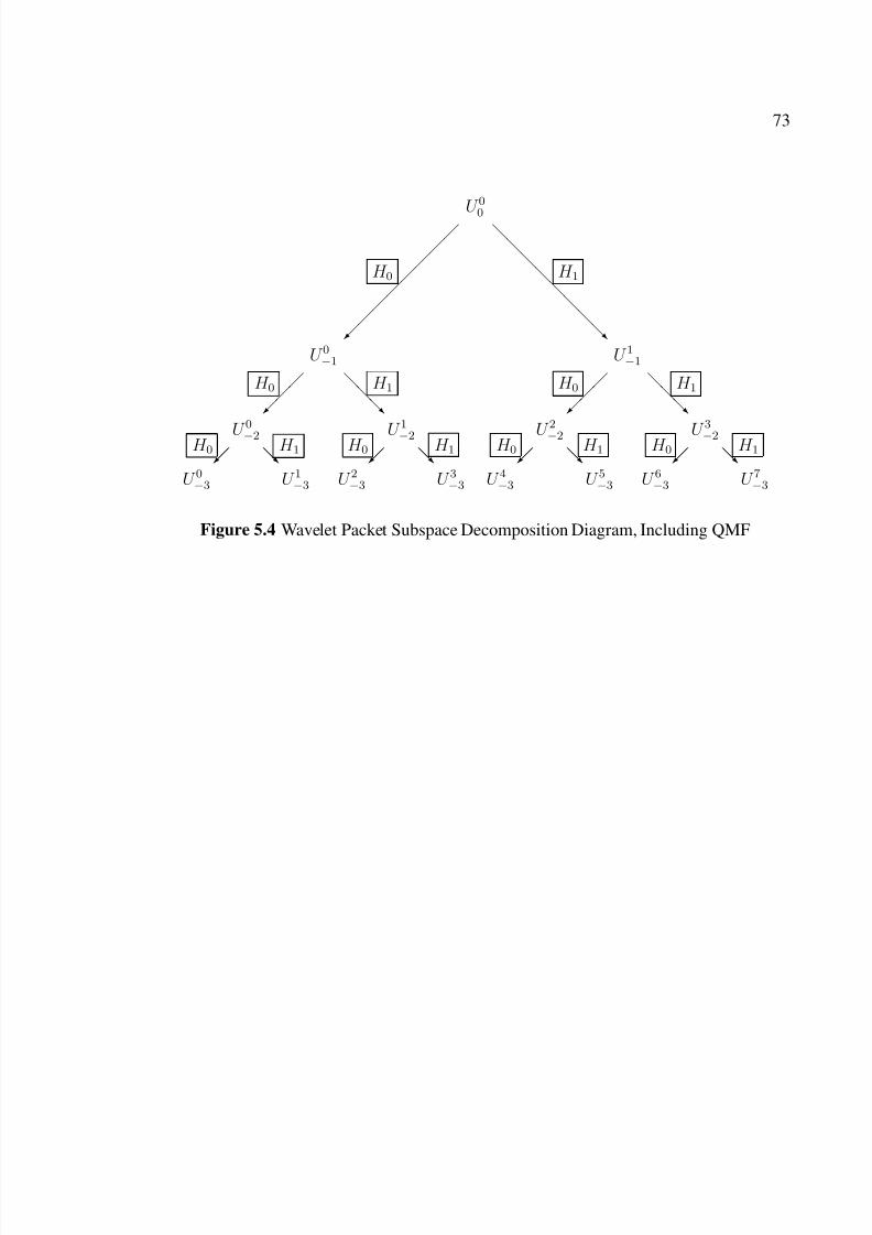
5.3 Wavelet Packets . . . . . . . . . . . . . . . . . . . . . . . . . . . . . . . . . . . . . . . . . . . . . . . . . . . . . . 72

5.3.1 De-Noising Using Wavelet Packet Entropy-Based Best Bases . . . 76

5.3.2 De-Noising by Thresholding the Wavelet Packet Coef£cients. . . . 77

5.4 Singularity Detection Using Wavelets . . . . . . . . . . . . . . . . . . . . . . . . . . . . . . . . .78

5.5 Detailed Listing of Algorithms . . . . . . . . . . . . . . . . . . . . . . . . . . . . . . . . . . . . . . . . 81

6 RESULTS . . . . . . . . . . . . . . . . . . . . . . . . . . . . . . . . . . . . . . . . . . . . . . . . . . . . . . . . . . . . . . . . . . 8 5

6.1 Results of Clutter-Reduction Techniques . . . . . . . . . . . . . . . . . . . . . . . . . . . . . .85

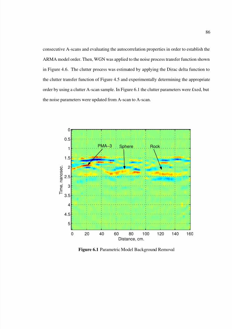
6.1.1 Model Estimated Background Removal .. . . . . . . . . . . . . . . . . . . . . . . 85

6.1.2 RLS Background Removal . . . . . . . . . . . . . . . . . . . . . . . . . . . . . . . . . . . . 87

6.2 Performance Measures of Clutter-Reduction Methods . . . . . . . . . . . . . . . . . . 88

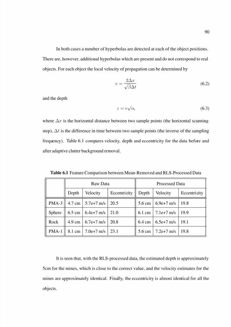
6.2.1 Physical Parameter Estimation. . . . . . . . . . . . . . . . . . . . . . . . . . . . . . . . .88

6.2.2 Target Class Discrimination . . . . . . . . . . . . . . . . . . . . . . . . . . . . . . . . . . .91

vii

7/29/2019 10.1.1.116.1392


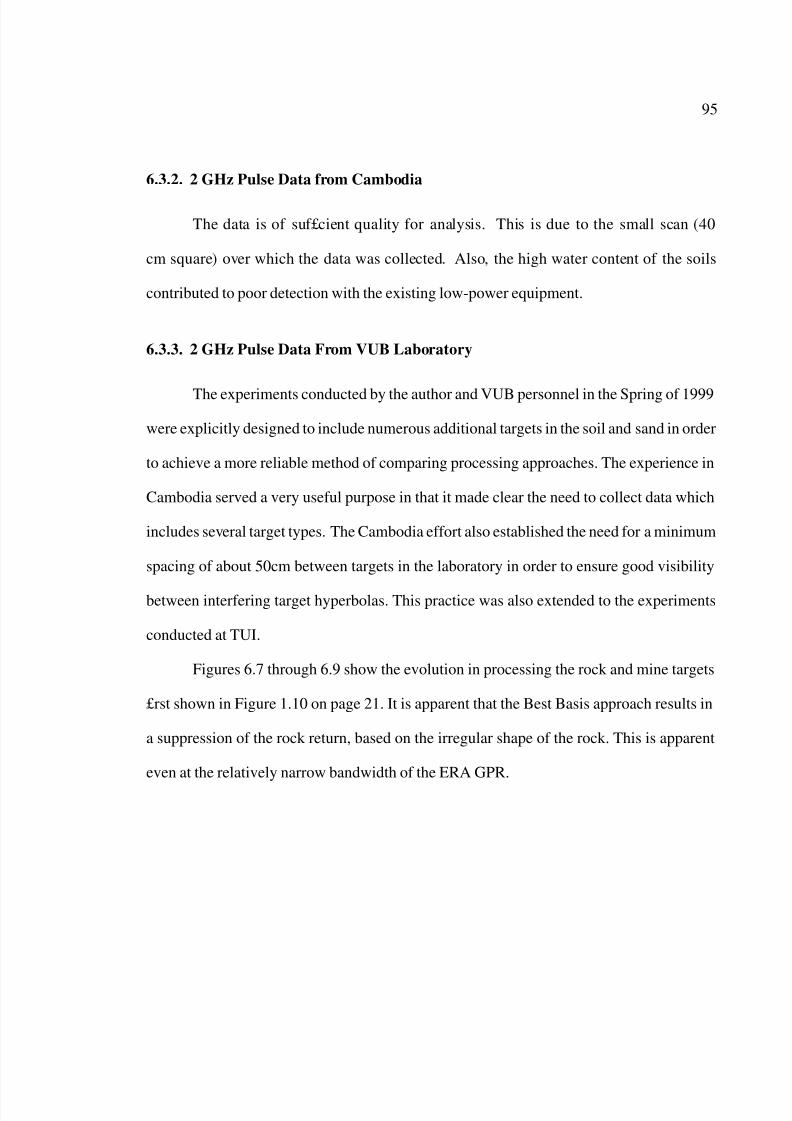
6.3 Results of Wavelet-Based Target Discrimination .. . . . . . . . . . . . . . . . . . . . . . 92

6.3.1 2 GHz Pulse Data From EPFL/DeTec Laboratory. . . . . . . . . . . . . . . 92

6.3.2 2 GHz Pulse Data from Cambodia . . . . . . . . . . . . . . . . . . . . . . . . . . . . .95

6.3.3 2 GHz Pulse Data From VUB Laboratory . . . . . . . . . . . . . . . . . . . . . . 95

6.3.4 6 GHz Data from TUI . . . . . . . . . . . . . . . . . . . . . . . . . . . . . . . . . . . . . . . . . 99

6.3.5 10 GHz Pulse Data From RMA . . . . . . . . . . . . . . . . . . . . . . . . . . . . . . . .100

7 SUMMARY OF CONTRIBUTIONS AND SUGGESTIONS FOR

FURTHER RESEARCH . . . . . . . . . . . . . . . . . . . . . . . . . . . . . . . . . . . . . . . . . . . . . . . . . . . . .104

7.1 Speci£c Contributions of This Dissertation .. . . . . . . . . . . . . . . . . . . . . . . . . . .104

7.2 Suggestions for Further Research . . . . . . . . . . . . . . . . . . . . . . . . . . . . . . . . . . . . .105

APPENDIX: SOME TYPICAL ANTI-PERSONNEL LAND MINES . . . . . . . . . . . . . . .107

REFERENCES. . . . . . . . . . . . . . . . . . . . . . . . . . . . . . . . . . . . . . . . . . . . . . . . . . . . . . . . . . . . . . . . . . . . . . . . . . . .120

viii

7/29/2019 10.1.1.116.1392


LIST OF FIGURES

1.1 Namibian Deminer in the Tall Grass, Clearing a Mine Lane . . . . . . . . . 6

1.2 Author Prodding for APL in Cambodia . . . . . . . . . . . . . . . . . . . . 6

1.3 Loss Tangent as Function of Gravimetric Water Content . . . . . . . . . . . 10

1.4 Real Part of Sand Permittivity as Function of Gravimetric Water Content . . 10

1.5 A-scan (Left) and B-scan (Right) Representations of GPR Data; T72 APL

in 5 cm Sand . . . . . . . . . . . . . . . . . . . . . . . . . . . . . . . . . 15

1.6 C-scan Representation of T72 APL in 5 cm Sand . . . . . . . . . . . . . . 16

1.7 GPR C-scan at 5.0 cm Depth . . . . . . . . . . . . . . . . . . . . . . . . . 19

1.8 Typical Battle£eld Clutter (False Targets) From Cambodia . . . . . . . . . 19

1.9 B-scan of Various Targets and Target Separation in Dry Sand . . . . . . . . 20

1.10 Comparison between Rock and Mine Targets . . . . . . . . . . . . . . . . 21

1.11 Clutter Limited Nature of the GPR Target . . . . . . . . . . . . . . . . . . 23

3.1 EPFL/DeTec Sandbox With SPRScan Radar . . . . . . . . . . . . . . . . . 29

3.2 Close-Up View of GPR Transmitter/Receiver Head . . . . . . . . . . . . . 29

3.3 Scanning Pattern of DeTec Laboratory SPRScan Radar . . . . . . . . . . . 30

3.4 DeTec-1 Handheld GPR In Croatia . . . . . . . . . . . . . . . . . . . . . . 31

3.5 Hand-held Scan Pattern, Viewed From Above. Dimensions are Millimeters 33

3.6 Location of Mine Fields, Thmar Pouk, Cambodia . . . . . . . . . . . . . . 34

3.7 Author Demining with Ebinger Metal Detector . . . . . . . . . . . . . . . 34

3.8 DeTec-2 Operation . . . . . . . . . . . . . . . . . . . . . . . . . . . . . . 36

3.9 DeTec-2 Scan Pattern . . . . . . . . . . . . . . . . . . . . . . . . . . . . . 37

3.10 Author’s Laptop, DeTec-2 in Background . . . . . . . . . . . . . . . . . . 37

3.11 Author Soaking Clay in Preparation for Experiments . . . . . . . . . . . . 39

ix

7/29/2019 10.1.1.116.1392


3.12 Target Set in VUB Lab, Dry Sand, Flat Surface; Multiple Objects to Present

Interfering Clutter . . . . . . . . . . . . . . . . . . . . . . . . . . . . . . . 40

3.13 Target Set in VUB Lab, Dry Sand, Flat Surface . . . . . . . . . . . . . . . 41

3.14 Target Set in VUB Lab, Wet Clay, Irregular Surface . . . . . . . . . . . . . 42

3.15 Target Set in VUB Lab, Dry Clay, Irregular Surface . . . . . . . . . . . . . 43

3.16 Magnitude Spectrum of Typical Scan at TUI . . . . . . . . . . . . . . . . . 45

3.17 Resultant A-scan, Time Domain . . . . . . . . . . . . . . . . . . . . . . . 45

3.18 Measurement Scenario at TUI Lab . . . . . . . . . . . . . . . . . . . . . . 46

3.19 Transmitted Waveform of RMA GPR . . . . . . . . . . . . . . . . . . . . 47

4.1 Overview of System Impulse Response . . . . . . . . . . . . . . . . . . . 50

4.2 Discrete LTI Block Diagram . . . . . . . . . . . . . . . . . . . . . . . . . 51

4.3 General Block Diagram Representation of System Identi£cation . . . . . . 52

4.4 Representation of Target Parametric Model . . . . . . . . . . . . . . . . . 53

4.5 Representation of Clutter Parametric Model . . . . . . . . . . . . . . . . . 54

4.6 Representation of Added Noise Parametric Model . . . . . . . . . . . . . . 55

4.7 B-scan of Copper Plate Buried 30cm in Sand . . . . . . . . . . . . . . . . 57

4.8 Result of Model-Based Clutter Removal . . . . . . . . . . . . . . . . . . . 57

5.1 Tilings of the Time-Frequency (Time-Scale) Plane . . . . . . . . . . . . . . 64

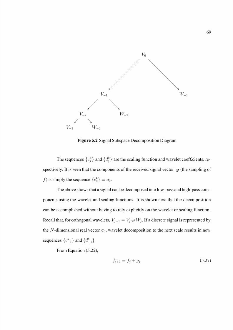
5.2 Signal Subspace Decomposition Diagram . . . . . . . . . . . . . . . . . . 69

5.3 Symbolic Representation of Wavelet Coef£cient Decomposition . . . . . . 71

5.4 Wavelet Packet Subspace Decomposition Diagram, Including QMF . . . . 73

5.5 Two-Channel QMF For Perfect Reconstruction . . . . . . . . . . . . . . . 74

5.6 Symbolic Representation of Wavelet Packet Coef£cient Decomposition . . 74

5.7 Wavelet Packet Best Basis Entropy Tree, Chirp Signal . . . . . . . . . . . . 75

5.8 Wavelet Packet Tiling of Time-Scale Plane . . . . . . . . . . . . . . . . . . 75

5.9 Wavelet Modulus Maxima (Bottom) of a Discontinuous Signal (Top) . . . . 80

x

7/29/2019 10.1.1.116.1392


5.10 Program Flow . . . . . . . . . . . . . . . . . . . . . . . . . . . . . . . . . 82

6.1 Parametric Model Background Removal . . . . . . . . . . . . . . . . . . . 86

6.2 RLS Background Removal . . . . . . . . . . . . . . . . . . . . . . . . . . 87

6.3 Detected Hyperbolas in Mean-Removed Background . . . . . . . . . . . . 89

6.4 Detected Hyperbolas RLS-Removed Background . . . . . . . . . . . . . . 89

6.5 PMN Mine, RLS Clutter Removal . . . . . . . . . . . . . . . . . . . . . . 93

6.6 PMN Mine, Wavelet-Detected . . . . . . . . . . . . . . . . . . . . . . . . 94

6.7 Rock and Mine . . . . . . . . . . . . . . . . . . . . . . . . . . . . . . . . 96

6.8 Rock and Mine, Clutter Removed . . . . . . . . . . . . . . . . . . . . . . 97

6.9 Best Basis Approach, Showing Suppression of False Target (Rock) . . . . . 98

6.10 Best Basis Results With TUI Frequency-Stepped GPR . . . . . . . . . . . 99

6.11 PMN Mine C-scan, Clutter Removed . . . . . . . . . . . . . . . . . . . . . 101

6.12 Best Basis Detected PMN Mine . . . . . . . . . . . . . . . . . . . . . . . 101

6.13 Stone, Clutter Removed . . . . . . . . . . . . . . . . . . . . . . . . . . . . 102

6.14 Best Basis Detected Stone . . . . . . . . . . . . . . . . . . . . . . . . . . 102

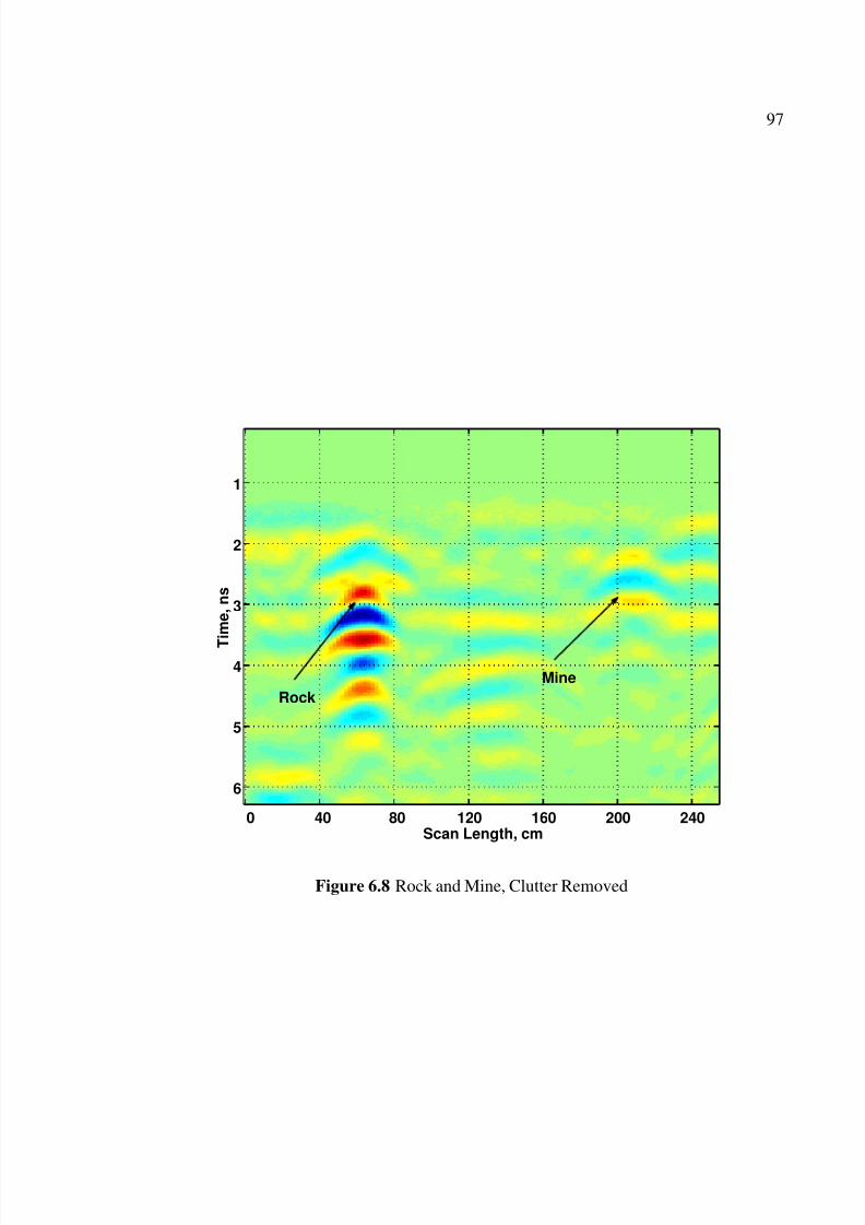
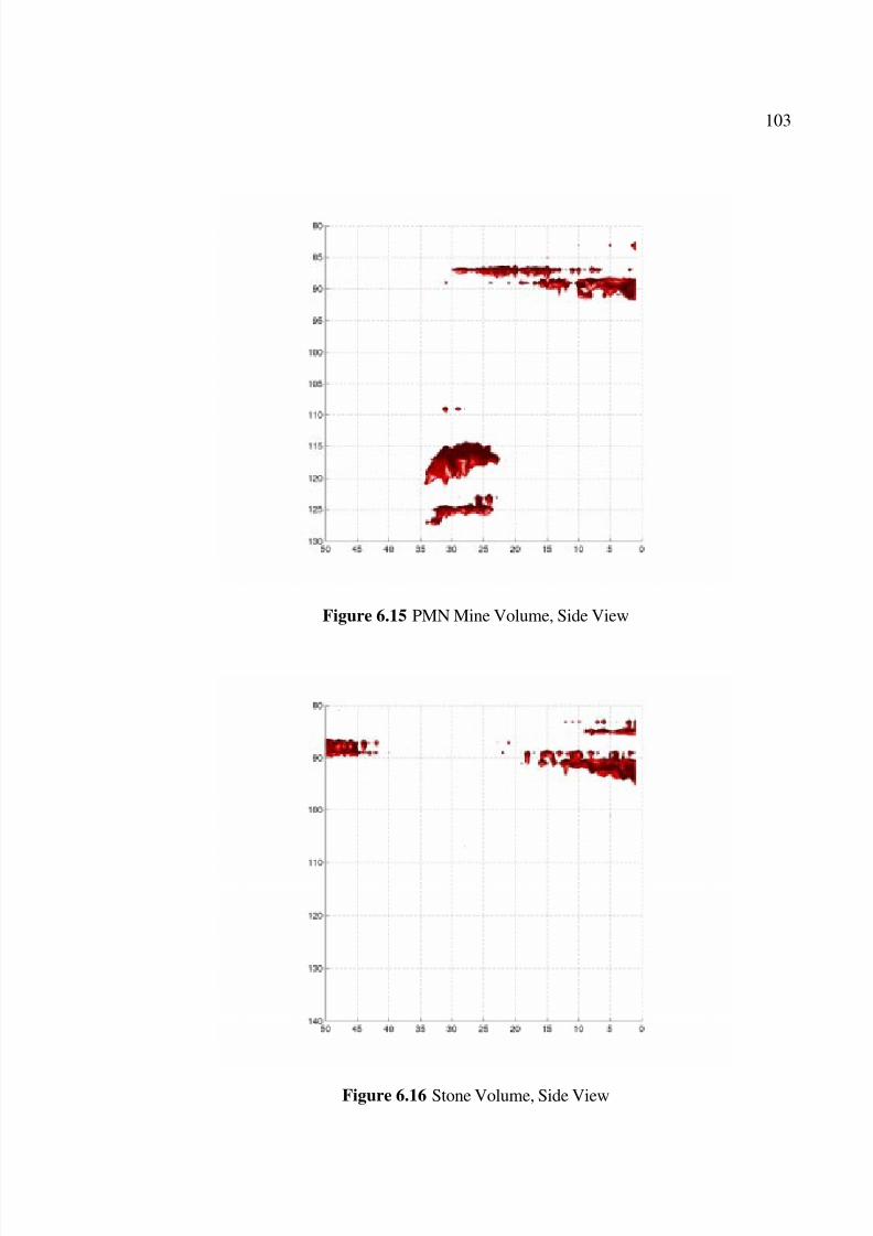
6.15 PMN Mine Volume, Side View . . . . . . . . . . . . . . . . . . . . . . . . 103

6.16 Stone Volume, Side View . . . . . . . . . . . . . . . . . . . . . . . . . . . 103

A.1 Chinese Type 72 APL . . . . . . . . . . . . . . . . . . . . . . . . . . . . . 108

A.2 Details of T72B, Anti-Handling Mechanism, from Sales Brochure . . . . . 108

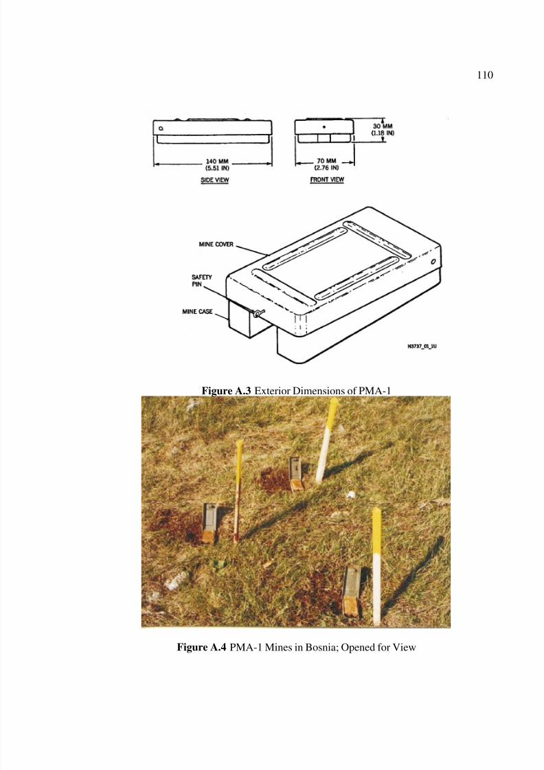
A.3 Exterior Dimensions of PMA-1 . . . . . . . . . . . . . . . . . . . . . . . . 110

A.4 PMA-1 Mines in Bosnia; Opened for View . . . . . . . . . . . . . . . . . . 110


A.6 Internal View of PMA-2 . . . . . . . . . . . . . . . . . . . . . . . . . . . 112


A.8 Internal View of PMA-3 . . . . . . . . . . . . . . . . . . . . . . . . . . . 114

A.9 Russian PMN-Type APL . . . . . . . . . . . . . . . . . . . . . . . . . . . 116

xi

7/29/2019 10.1.1.116.1392


A.10 PMN Details . . . . . . . . . . . . . . . . . . . . . . . . . . . . . . . . . 116

A.11 Yugoslav PMU Series Mine . . . . . . . . . . . . . . . . . . . . . . . . . . 117

A.12 Example of Wooden Box Mine . . . . . . . . . . . . . . . . . . . . . . . . 117

A.13 U.S. M-14 APL . . . . . . . . . . . . . . . . . . . . . . . . . . . . . . . . 119

A.14 U.S. M-14 APL, Details . . . . . . . . . . . . . . . . . . . . . . . . . . . 119

xii

7/29/2019 10.1.1.116.1392


LIST OF TABLES

1.1 Top 12 Mined Countries . . . . . . . . . . . . . . . . . . . . . . . . . . . 5

1.2 Polynomial Coef£cients for Equation (1.8) . . . . . . . . . . . . . . . . . . 11

1.3 Electrical Properties of APL Explosives and Explosive Simulants . . . . . . 12

1.4 Attenuation of Electromagnetic Waves in Sand (dB/m) . . . . . . . . . . . 13

1.5 Attenuation of Electromagnetic Waves in Silt (dB/m) . . . . . . . . . . . . 13

6.1 Feature Comparison between Mean-Removed and RLS-Processed Data . . 90

6.2 Comparison Results Based on Feature Selection . . . . . . . . . . . . . . . 91

xiii

7/29/2019 10.1.1.116.1392


LIST OF SYMBOLS

Symbol Meaning Value/Units

Z+ Positive Integers –

R Real Numbers –

C Complex Numbers –

∈ Subset –

(Wxf ) Continuous Wavelet Transform

C Speed of Light 2.99792458 × 108m/s

µ0 Permeability of Free Space 4π × 10−7Sec Volt

Amp Meter

ε0 Permittivity of Free Space 8.85419 10−12Amp Sec

Meter Volt

η Intrinsic Impedence Ohm

α Attenuation Constant1

m

β Phase Constantrad

m

γ Propagation Constant α + iβ

∗ Linear Convolution –

ϕ(t) Scaling Function –

x(t) Wavelet Function –

{q k} High-Pass (Wavelet) Filter Coef£cients –

⊕ Orthogonal Sum –

V j Approximation Subspace –

Ψ ,Q ,P ,R Matrix Notation –

k Vector Notation –

W, V Wavelet and Scaling Function Subspaces –

xiv

7/29/2019 10.1.1.116.1392


Symbol Meaning Value/Units

U n j Wavelet Packet Subspace at Scale j –

B Orthonormal Wavelet Packet Basis Library –

i Imaginary Number√ −1

i,j,k,l Indices –

e Exponential Operator –

u(n) nth Discrete Input Sample –

y(n) nth Discrete Output Sample –

h(n) Discrete Impulse Response

Rν (k) Autocovariance Function –

φuu Autocorrelation Function –

φuy Crosscorrelation Function –

xv

7/29/2019 10.1.1.116.1392


CHAPTER 1

INTRODUCTION

Antipersonnel land mines (APL’s) remain hidden in the ground in over 64 coun-

tries following the termination of armed con¤ict [1]-[3]. The exact number of APL’s is not

known [4]; indeed, the number of APL’s is rather irrelevant. The fact remains that APL’s

account for hundreds of civilian casualties per year and prevent the return of land to agri-

cultural use.1 The standard approach to the detection of APL’s remains the metal detector

(MD) which is essentially unchanged from the approach used in World War II. Because a

large number of APL’s contain little to no metal, ground penetrating radar (GPR) is one

of the current technologies which is receiving attention as an alternative or adjunct to the

metal detector.

This dissertation addresses the two main challenges in detecting small buried APL’s

which contain little or no metal: soil clutter-reduction and mine feature extraction. Non-

metal (NM) and minimum-metal(MM) APL’s remain an extremely lethal threat to millions

of innocent civilians throughout dozens of post-con¤ict countries. The need to develop

ef£cient methods of £nding the mines is compelling; such a method or system of methods

has not been developed to date in spite of tens of millions of dollars invested by numerous

governments.

1

The author personally observed the effects of APL’s on the local populace in Cambodia and Croatia in1997.

1

7/29/2019 10.1.1.116.1392


2

Various GPR devices have been developed, including vehicle-mounted, hand-held

and airborne. None of these systems works well enough to be deployed to a real mine£eld.

In the “real world” the ubiquitous metal detector and prodding stick remain the tools of

the trade. While we can visually observe galaxies millions of light years away, peer into

the depths of the ocean and use radar to track small objects at thousands of kilometers, we

cannot reliably locate APL’s only centimeters beneath our feet. The reasons are many:

(i) The soil surface presents a severe clutter environment to the GPR waveform. Of-

ten, the radar sensor is placed 10-15 cm above the soil surface, and antenna-soil

interactions create additional clutter and cross-talk.

(ii) The radar waveform may not be of suf£cient bandwidth to permit resolution of the

mine target from other non-lethal targets such as rocks, roots, etc.

(iii) Signal processing methods have not been developed which can exploit the internal

structures of man-made objects (mines) and which will reject natural objects (rocks)

which might otherwise appear as valid mine targets.

Item (ii) above is the subject of much research in the demining community; the test

facilities used for this dissertation did not always have suf£cient bandwidth, but were the

only ones available to the author. A notable exception was 10 GHz data made available

to the author towards the end of this research, and the results of processing these data are

included here.

1.1. Objectives

The broad objective of this research was to develop new and innovative signal pro-

cessing techniques to improve the detectability of buried anti-personnel land mines (APL’s)

using ground penetrating radar (GPR). This dissertation focuses on items (i) and (iii) above.

7/29/2019 10.1.1.116.1392


3

The author developed a set of adaptive clutter-reduction techniques [5] while working at

the Vrije Universiteit Brussel (VUB) under the direction of Prof. Hichem Sahli; funding

was provided by a grant from the European Union (EU) as part of the EU humanitarian

demining research project DEMINE. Clutter-reduction is, however, a tool to be used in the

next step, item (iii), APL shape feature determination. This series of techniques relies on

the observation that all existing APL’s have some regular shape, either cylindrical or box-

shaped. In either case, ¤at surfaces exist which may provide information to the radar that

a man-made object is the target, and not simply a false target made up of many random

scatterers such as shrapnel, rocks, etc.

Chapter 2 describes the state-of-the-art and on-going research programs at various

universities and within various governments. The data sources for this dissertation are

described in Chapter 3 and consist of both laboratory and £eld tests, many of which the

author participated in and conducted. The technical details for system identi£cation and

the application to clutter characterization and reduction are provided in Chapter 4. Chapter

5 describes the fundamental properties of wavelets and wavelet packets in signal decom-

position and singularity detection, and the application to detecting the APL. Chapter 6

summarizes the results of the developed methods using various data from the data sources.

Chapter 7 summarizes the contributions of the current research and suggests topics for ad-

ditional follow-on research. Finally, the Appendix describes some typical APL’s which are

threats to populations around the world and were used in the research described here.

1.2. Background

The purpose of anti-personnel land mines (APL’s) is to kill or maim members of an

opposition force during combat. Because APL’s remain active for many decades following

a con¤ict, they prove devastating for civilians who are trying to reclaim their land. Personal

7/29/2019 10.1.1.116.1392


4

observations of mined residential areas in Karlovac, Croatia and Thmar Pouk, Cambodia in

1997 reveal a severe limitation of activities in which the locals are able to participate. The

majority of mined areas are discovered only after a civilian has been killed or maimed from

a mine accident; in time, the land reverts to a heavily overgrown state making detection

and removal of the land mines even more dif£cult. Efforts follow to localize the mined

areas and locate and clear individual mines. Currently, only hand-held metal detectors are

used in most humanitarian demining operations. The metal detector is extremely reliable,

but also extremely slow. Also, the metal detector produces a considerable number of false

alarms, sometimes even alarming on apparently non-metallic clutter such as some rocks

and soils.2 Testimonials from deminers in the £eld indicate that only about 100 m2 can be

cleared per day. This is due to the signi£cant amount of metallic clutter present in a typical

post-con¤ict area.

Although the number of post-con¤ict APL’s throughout the world is not known

exactly, the UN and US State Department have estimated that there are between 64 million

and 110 million scattered throughout 64 countries in which con¤ict has ceased [1]-[3];

Table 1.2 lists the top 12 mined countries according to the UN data base (UNLDB) and the

State Department 1998 survey Hidden Killers 98 [2].

The mine detection equipment used for humanitarian demining is often constrained

to be portable, and while the indigenous operator is usually well-trained, he is limited in

his ability to operate high-tech equipment; thus, any detection/classi£cation device must

present the operator with unambiguous information. Signal and image processing algo-

rithms used for such demining must aid the operator in achieving very high levels of detec-

tion, currently 99.6 to 99.9% [6], [7]. False alarm rates must also be reduced. False alarm

rates in Afghanistan, for example, using standard manual demining techniques, approach

2Indeed, the author’s personal experiences in Cambodia indicate that, in such a highly metallic soil "lat-

terite," the metal detector can be rendered almost useless.

7/29/2019 10.1.1.116.1392


5

Table 1.1 Top 12 Mined Countries

Country UNLDB HK98 Case Study

Low High

Afghanistan 10,000,000 5,000,000 7,000,000

Angola 15,000,000 6,000,000 15,000,000

Bosnia-Herzegovina 3,000,000 600,000 1,000,000

Cambodia 6,000,000 4,000,000 6,000,000

Croatia 3,000,000 400,000 400,000

Eritrea 1,000,000 500,000 1,000,000Iraq (Kurdistan) 10,000,000 10,000,000 10,000,000

Mozambique 3,000,000 1,000,000 1,000,000

Namibia 50,000 50,000 50,000

Nicaragua 108,297 85,000 85,000

Somalia 1,000,000 1,000,000 1,000,000

Sudan 1,000,000 1,000,00 1,000,000

TOTAL 53,158,297 29,635,000 43,535,000

1,000:1 [8]. Personal experience by this author in Cambodia con£rms this statement; the

vast majority of time is spent in detecting/removing shrapnel and other non-lethal debris.

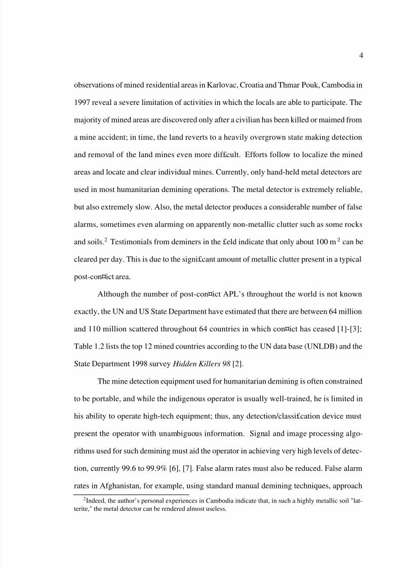
The current method of demining is quite simple, effective, but very slow. Figure

1.1 shows the environment in many parts of the world. Once an area is mined, grass and

other shrubbery rapidly cover the area and must be removed, often by hand. The £gure

illustrates the common method of searching for mines with a metal detector. The deminer

operates within a lane approximately 1 meter wide as indicated by the strips of cloth on

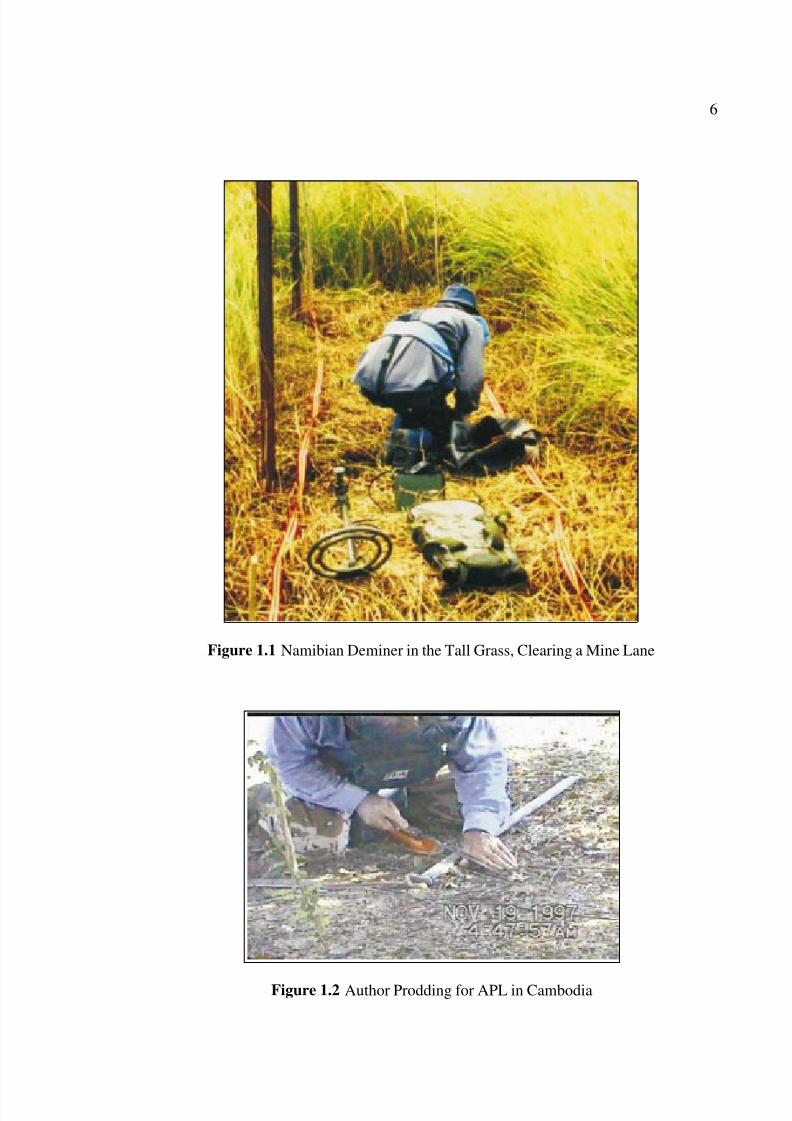
either side of the deminer. Figure 1.2 shows the author in Cambodia, demonstrating the

prodding technique; the 1 meter wooden stick denotes the boundary of the cleared lane.

7/29/2019 10.1.1.116.1392


6

Figure 1.1 Namibian Deminer in the Tall Grass, Clearing a Mine Lane

Figure 1.2 Author Prodding for APL in Cambodia

7/29/2019 10.1.1.116.1392


7

1.3. GPR As a Detector for Buried Objects

In order to establish the principles of GPR applied to the detection of buried ob-

jects, it is £rst necessary to review the electromagnetic properties of soils and the objects

themselves.

1.3.1. Electromagnetic Properties of Soil and Nonmetallic Mines

The interaction of an electromagnetic wave with the soil is a complex function of

frequency, soil type and water content [9],[10]. In the following, a linearly polarized,

plane wave 3 is assumed passing from medium 1 characterized by {µ1, ε1, σ1} to medium

2 characterized by {µ2, ε2, σ2}, where µ is the permeability, ε is the permittivity and σ is

the conductivity of the medium.

The solution of Maxwell’s equations in one dimension and at a single frequency ω

is shown in any elementary textbook on electromagnetics [11] to be

E (z, t) = E 0eiωt−γz , (1.1)

where E 0 is the amplitude of the electric £eld at the origin (z = 0) and γ is the propagation

constant

γ = α + iβ = iω µε1

−iε

ε , (1.2)

where ε and ε are the real and imaginary parts, respectively, of the complex permittivity

ε. The ratio ε

εis called the loss tangent , denoted by tan δ . The complex permittivity ε is

the product of the relative permittivity of the medium εr and the permittivity of free space

ε0, ε = ε0εr, where

ε0 = 8.854

×10−12

≈

1

36π ×10−9 F/m.

3In practice, the size of a typical antenna and the height above the ground (about 10 cm) results in a

spherical wave; a plane wave is assumed here for clarity of illustration.

7/29/2019 10.1.1.116.1392


8

In a similar manner, the permeability µ is the product of the relative permeability µr of the

medium and the permeability of free space µ0, µ = µrµ0, where

µ0 = 4π × 10−7 H/m;

for dielectrics, µr = 1. Some soils such as that found in parts of Cambodia (“latterite”)

have non-unity relative permeability.

The attenuation constant α and the phase constant β are then

α = ω

µε

2

1 +

ε

ε

2

− 1

1

2

m−1 (1.3)

β = ω

µε

2

1 +

ε

ε

2

+ 1

12

rad

m. (1.4)

The velocity of wave propagation in the medium, for tan δ 1 is shown in Coifman and

Wickerhauser [12] to be

v ≈ c√ εr

, (1.5)

where c is the velocity of light in free space, c ≈ 3× 108 m/s.

The intrinsic impedence η is given by

η =

µ

ε

1 − iε

ε

Ohms, (1.6)

and the power re¤ected at the interface between two layers with different properties (such as

the boundary between the soil and the APL) is given by the re¤ection coef£cient r denoted

by the ratio of the re¤ected power Pr to the incident power Pi [11]

r =Pr

Pi

=η2 − η1η2 + η1

, (1.7)

where the direction of propagation is assumed to be from medium 1 to medium 2. In the

case of medium 2 being a perfect conductor (such as a metallic APL), the re¤ected power

equals the incident power.

7/29/2019 10.1.1.116.1392


9

At the interface, the re¤ected wave also undergoes a phase shift, or phase disconti-

nuity. It is this discontinuity which is exploited for detecting the soil-mine interface.

The amount of re¤ected power is seen from Equation (1.7) to be a function of the

intrinsic impedence which is, in turn, a function of the relative permittivities between the

two media; the “contrast” between the soil and the buried object will therefore be enhanced

if there is a wide disparity between the permittivities of the soil and mine.

The Université Catholique de Louvain (Belgium) conducted an extensive series of

tests on soil samples from various test ranges in 1997 [9]. Plots of the loss tangent and

relative permittivity of selected sand and silty soil samples are shown in Figures 1.3 and

1.4, respectively, for 2 GHz and 10 GHz. The polynomial

f (cw) = α3c3w + α2c2w + α1cw + α0, (1.8)

where f (cw) represents either of ε, εε 2GHz

or εε 10GHz

from Table 1.2 can be used to

approximate the values for loss tangent and attenuation for both sand and silt at 2.0 and

10.0 GHz. The variable cw represents the gravimetric water content of the soil in percent.

7/29/2019 10.1.1.116.1392


10

0 5 10 15 200

0.05

0.1

0.15

0.2

0.25

0.3

0.35

0.4

Percent Water Content

t a n δ

10 GHz

2 GHz

Figure 1.3 Loss Tangent as Function of Gravimetric Water Content

0 5 10 15 202

4

6

8

10

12

14

16

18

Percent Water Content

ε

′

10 GHz

2 GHz

Figure 1.4 Real Part of Sand Permittivity as Function of Gravimetric Water Content

7/29/2019 10.1.1.116.1392


11

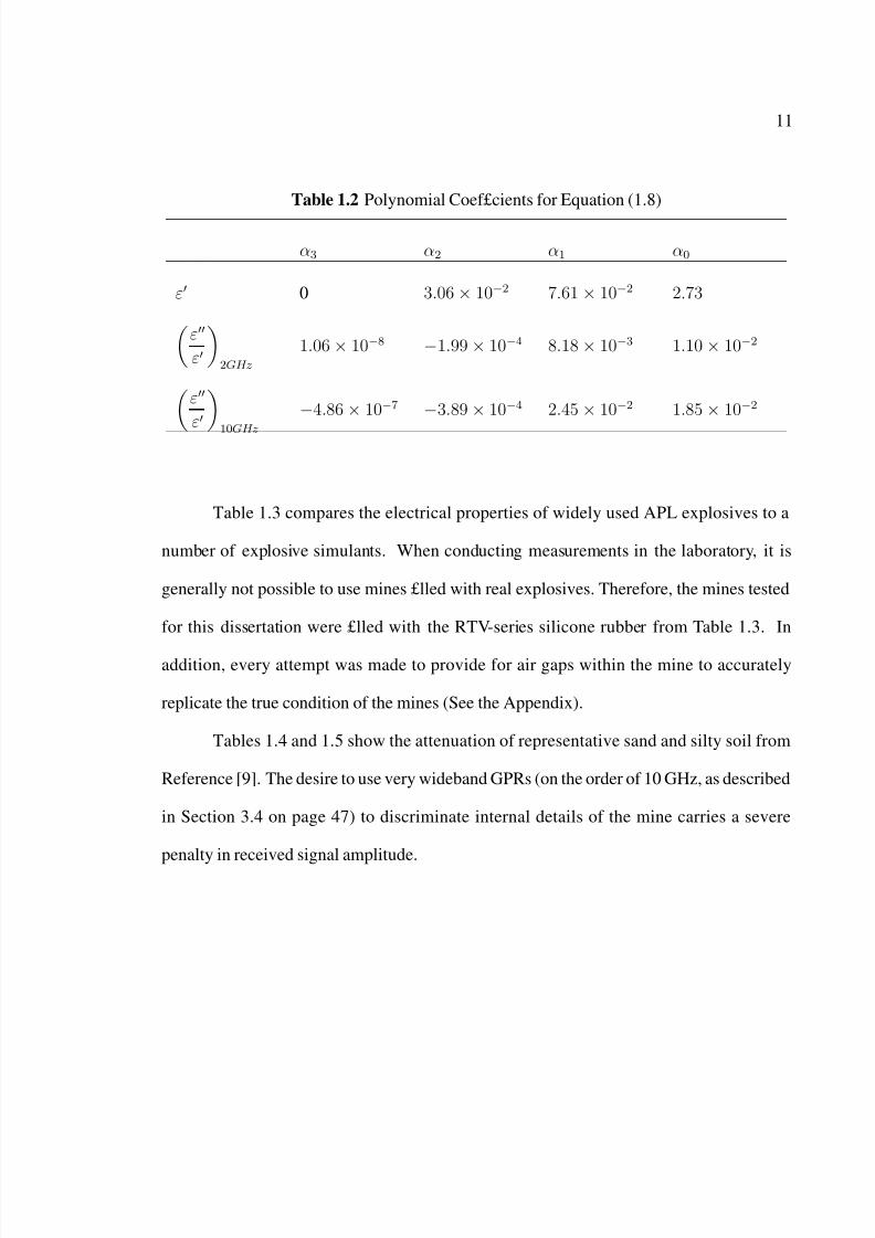
Table 1.2 Polynomial Coef£cients for Equation (1.8)

α3 α2 α1 α0

ε 0 3.06 × 10−2 7.61 × 10−2 2.73ε

ε

2GHz

1.06 × 10−8 −1.99 × 10−4 8.18 × 10−3 1.10 × 10−2

ε

ε 10GHz

−4.86 × 10−7 −3.89 × 10−4 2.45 × 10−2 1.85 × 10−2

Table 1.3 compares the electrical properties of widely used APL explosives to a

number of explosive simulants. When conducting measurements in the laboratory, it is

generally not possible to use mines £lled with real explosives. Therefore, the mines tested

for this dissertation were £lled with the RTV-series silicone rubber from Table 1.3. In

addition, every attempt was made to provide for air gaps within the mine to accurately

replicate the true condition of the mines (See the Appendix).

Tables 1.4 and 1.5 show the attenuation of representative sand and silty soil from

Reference [9]. The desire to use very wideband GPRs (on the order of 10 GHz, as described

in Section 3.4 on page 47) to discriminate internal details of the mine carries a severe

penalty in received signal amplitude.

7/29/2019 10.1.1.116.1392


12

Table 1.3 Electrical Properties of APL Explosives and Explosive Simulants

Frequency

Material 0.3 GHz 1.0 GHz 3.0 GHz

εr tan δ εr tan δ εr tan δ

TNT 2.89 0.0039 – – 2.89 0.0018

Composition B 3.20 0.0035 – – 3.20 0.0020

RTV-3112 3.13 0.0036 3.32 0.0155 – –

RTV-3110 2.88 0.0016 2.97 0.0084 – –

Nylon 3.08 0.0138 – – – –

ABS Plastic 2.67 0.0285 2.91 0.0784 – –

Paraf£n Wax 2.20 0.0203 – – – –

Source: EPFL/DeTec

7/29/2019 10.1.1.116.1392


13

Table 1.4 Attenuation of Electromagnetic Waves in Sand (dB/m)

Gravimetric Frequency

Water Content, % 2 GHz 4 GHz 6 GHz 8 GHz 10 GHz 12 GHz

0 1 3 10 20 32 48

5 15 48 99 189 25 336

10 33 106 218 396 537 714

15 54 171 358 628 870 1166

20 73 233.92 498 842 1205 1650

Table 1.5 Attenuation of Electromagnetic Waves in Silt (dB/m)

Gravimetric Frequency

Water Content, % 2 GHz 4 GHz 6 GHz 8 GHz 10 GHz 12 GHz

0 5 – 23 23 23 24

5 19 – 99 150 210 300

10 36 – 194 394 474 655

15 55 – 295 592 832 1097

20 71 – 374 909 1262 1578

7/29/2019 10.1.1.116.1392


14

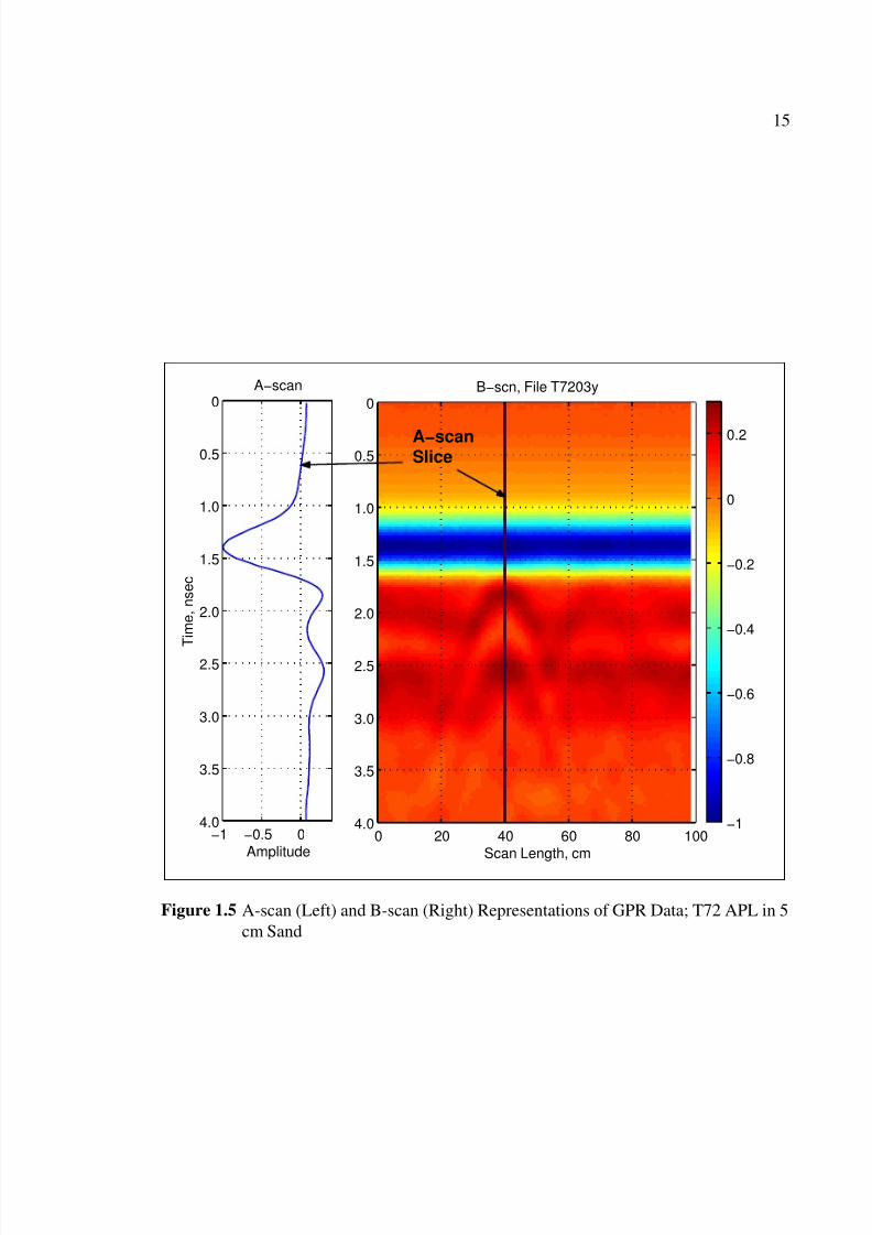
1.3.2. Types of GPR Scans

For a complete understanding of the terminology used in the GPR and demining

communities, the types of data representations are the A-scan, B-scan and the C-scan.

A-scan and B-scan The A-scan is a time-amplitude plot and represents a single pulse

return with the GPR antenna at a speci£c location above the ground. The B-scan represents

a series of A-scans as the GPR is swept in a straight line above the ground, at a constant

height. Figure 1.5 illustrates the concept. The ground clutter return is shown as a blue

band in the B-scan and is represented by the large negative swing of the A-scan. The

target location (in this case, a T72 APL buried 5 cm in sand) is roughly identi£ed by the

dim hyperbolic traces at the scan distance of 40 cm in the B-scan. The ground return is

much larger than the target return and must be removed. Typically, this is accomplished by

removing an average background, but this does not work well if the ground is anything but

perfectly ¤at and the GPR is not moved in a perfectly horizontal direction. (The APL data

presented here is from lab measurements at EPFL.)

C-scan The C-scan is represented by a horizontal slice of a number of stacked B-scans.

Figure 1.6 illustrates the situation with the T72 APL. In this £gure, the average background

has been removed and the target shows up as a “wave-like” structure. This appearance is

typical of GPR C-scans regardless of the target; there is no useful information in this struc-

ture to aid in target identi£cation. This is because, in this case, the GPR has a bandwidth of

only 2 GHz, which is too narrow for frequency-based or even time-scale based methods.

7/29/2019 10.1.1.116.1392


15

−1 −0.5 04.0

3.5

3.0

2.5

2.0

1.5

1.0

0.5

0

Amplitude

T i m e , n s e c

A−scan

−1

−0.8

−0.6

−0.4

−0.2

0

0.2

Scan Length, cm

B−scn, File T7203y

0 20 40 60 80 100

0

0.5

1.0

1.5

2.0

2.5

3.0

3.5

4.0

A−scanSlice

Figure 1.5 A-scan (Left) and B-scan (Right) Representations of GPR Data; T72 APL in 5

cm Sand

7/29/2019 10.1.1.116.1392


16

0

10

20

30

40

0

10

20

30

40

50

60

70

80

90

100

−0.5

0

0.5

Scan Width, cm

C−ScanFiles: T72

Time Slice: 2.225ns

Scan Length, cm

Figure 1.6 C-scan Representation of T72 APL in 5 cm Sand

7/29/2019 10.1.1.116.1392


17

1.4. The Technical Challenges: Clutter and False Targets

Detecting and classifying nonmetallic (NM) and minimum-metal (MM) mines buried

in sand and soil offers considerable challenges for signal processing algorithms. Typically,

APL’s are buried less than 5 cm below the surface of the ground; this ensures that the

mine is hidden, while being close enough to the surface to permit the force of a footstep to

detonate the mine. Typical forces required range from 10 to 15 Kg, although some more

modern mines require a pressure of only 3 Kg for detonation. The clutter background is

severe and the medium is lossy and may be dispersive [13].

Technical means of detecting buried objects have shown a consistently poor ability

to classify the object into categories of threatening and non-threatening objects. For exam-

ple, three Advanced Technology Demonstrations (ATDs) for unexploded ordnance (UXO)

detection conducted at the U.S. Jefferson Proving Ground (JPG) between 1994 and 1997

showed “In general, demonstrators lack a capability to distinguish ordnance and the em-

placed nonordnance...” [14]. A survey of various commercially-available GPR consistently

reported that all failed to provide acceptable detection performance against minimum-metal

APL’s [15].

Detection of buried objects with a GPR is rather simple; almost anything under

the surface of the ground presents a return signal which may be confused with a valid

(lethal) target. In this regard, the characterization of the radar returns in the context of

the environment is essential. It is not suf£cient to say that “something” is buried...rather,

in humanitarian demining, it is mandatory that a lethal target be detected with nearly 100

percent reliability in any soil type.4

4In the context of decision theory, the cost of a “false rejection” (Type II error [16]) is extremely high, as

this would result in a true mine being overlooked with the consequences that the deminer would be injured

or killed. This leads one to the conclusion that we should seek to maximize the probability of detectionwhile simultaneously minimizing the probability of false rejection. In other words, set the decision threshold

arbitrarily high. This is, of course, untenable, so we must be willing to accept some level of risk.

7/29/2019 10.1.1.116.1392


18

For this research, three distinct types of radar (GPR) return are de£ned:

1. Target return which contains information about a Mine Target,

2. Target return which contains information about a Non-Mine Target but which may

be confused as a mine, and

3. Clutter returns caused by inhomogeneous soil and small metallic fragments which

may not be confused with a valid mine target, and antenna effects (See Section 4.1

on page 48).

1.4.1. Near-Surface Clutter

The clutter environment within the £rst few cm of the soil surface exhibits strong

radar re¤ections with highly non-stationary statistics. This is illustrated in Figure 1.75,

which shows the radar returns at a depth of 5.0 cm following mean background clutter

removal. The mines and other targets are placed in accordance with the test protocol the

author developed for the EU humanitarian demining project DEMINE, and is further ex-

plained in Chapter 6; the mine types used are described in the Appendix.

It can be seen that the clutter environment close to the surface is highly variable and

exhibits a varying texture, even after a signi£cant amount of background has been removed.

An example of metallic clutter which causes false alarms with both the metal detector and

the GPR is shown in Figure 1.8.

5In these £gures, and many others in this dissertation, the annotations refer to speci£c data £les or test

scenarios described in Chapter 3.

7/29/2019 10.1.1.116.1392


19

0

20

40

0

40

80

120

160

200

0

40

80

120

160

−1

0

1

File f3049004, Slice Number 95, Time Slice 1.9792 ns.

PMA−3

Sphere

Rock

PMA−1

Figure 1.7 GPR C-scan at 5.0 cm Depth

Figure 1.8 Typical Battle£eld Clutter (False Targets) From Cambodia

7/29/2019 10.1.1.116.1392


20

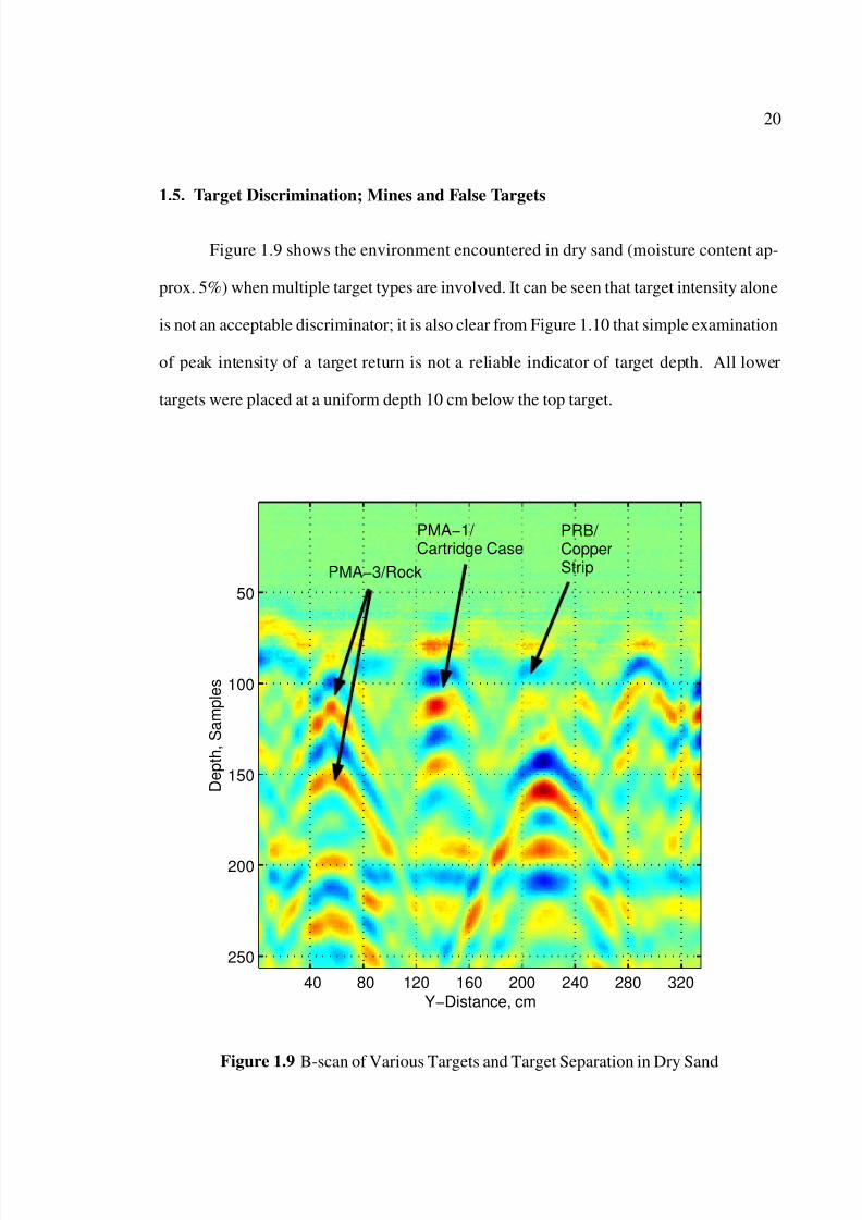
1.5. Target Discrimination; Mines and False Targets

Figure 1.9 shows the environment encountered in dry sand (moisture content ap-

prox. 5%) when multiple target types are involved. It can be seen that target intensity alone

is not an acceptable discriminator; it is also clear from Figure 1.10 that simple examination

of peak intensity of a target return is not a reliable indicator of target depth. All lower

targets were placed at a uniform depth 10 cm below the top target.

Y−Distance, cm

D e p t h , S a m p l e s

40 80 120 160 200 240 280 320

50

100

150

200

250

PMA−3/Rock

PMA−1/ Cartridge Case

PRB/ CopperStrip

Figure 1.9 B-scan of Various Targets and Target Separation in Dry Sand

7/29/2019 10.1.1.116.1392


21

X−Dimension, cm

D e p t h , S

a m p l e s

20 40 60 80 100 120

50

100

150

200

250

RockPMA−3 Mine

Figure 1.10 Comparison between Rock and Mine Targets

7/29/2019 10.1.1.116.1392


22

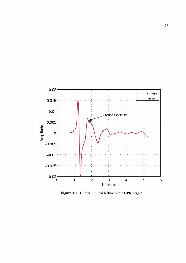
1.5.1. Signal-to-Noise Ratio (SNR) and Signal-to-Clutter Ratio (SCR)

Although expressions for the SCR of buried targets are available [17],[18], they do

not lend themselves well to the mine detection problem. This is because, for each time-

slice of the C-scan, the particular unit volume scatterer used for the comparison between

target energy and clutter energy varies greatly over the target location. In the raw, unpro-

cessed data, the target return is quite small compared to the background clutter, as shown in

Figure 1.11. Dif£culties arise because, in general, the actual “noise” (in the sense of zero-

mean White Gaussian Noise (WGN)) in the radar data is quite small because some form

of integration is used in all data considered here. The dominant interference in each of the

scan representations is correlated clutter, that is, interference which has a large correlation

coef£cient for lags greater than zero. A spectral decomposition of the mine return as in

Figure 1.11, for example, fails to reveal much about any “signal component” because the

residual clutter has essentially identical spectral characteristics as the signal itself. There-

fore, clutter-reduction methods are evaluated in the context of improvements in feature

extraction or classi£cation performance in Section 6.2 on page 88.

7/29/2019 10.1.1.116.1392


23

0 1 2 3 4 5 6−0.02

−0.015

−0.01

−0.005

0

0.005

0.01

0.015

0.02

Time, ns.

A m

p l i t u d e

cluttermine

Mine Location

Figure 1.11 Clutter Limited Nature of the GPR Target

7/29/2019 10.1.1.116.1392


CHAPTER 2

PREVIOUS RESEARCH

2.1. Survey of US Government and University Research

In February 1999, the author completed a comprehensive review of applicable US

humanitarian demining technology programs in cooperation with the EU DEMINE Project.

The US Government point of contact for all humanitarian demining programs is the Night

Vision Electronic Sensors Directorate (NVESD) of the US Army Night Vision Laboratory

(NVL) at Ft. Belvoir, VA. A supporting organization for test and evaluation is the Unex-

ploded Ordnance Center of Excellence (UXOCOE).

For this dissertation, each US humanitarian demining GPR program was reviewed;

the vehicular-mounted Ground-based STAnd-off Mine Detection System (GSTAMIDS),

the Hand-held STAnd-off Mine Detection System (HSTAMIDS), and a developmental

short-pulse GPR designated as the Wichmann radar [19]. In general, the tendency to em-

ploy stepped-frequency modulation is consistent between the three main programs; the

Wichmann radar uses a more conventional short-pulse modulation and very lossy horn an-

tennas, albeit a wideband pulse, ca. 5 GHz. Although no speci£c information was obtained

regarding signal processing methods and algorithms due to company proprietary consid-

erations, a review of applicable published literature and discussions with US Government

personnel revealed that, in general, the features used for classi£cation are rather simple, in-

24

7/29/2019 10.1.1.116.1392


25

cluding the statistical mean and variance of the returned signals under the assumption of a

Gaussian distribution for noise. This may explain in part the poor performance (at the time

of the survey) of the HSTAMIDS candidates to date. The US requirement for HSTAMIDS

is a probability of detection, Pd, of a mine to be 0.80; the best performance with trained

contractor personnel was 0.70, and the average performance using military personnel was

only 0.30 for min-metal APL.

Several universities are involved in mine detection research, and their journal papers

are included in the literature search here. Predominant universities are Duke and Ohio State

in the US and the VUB and TUI in Europe.

2.2. Results of Technology Literature Search

A basic tutorial on GPR is provided by Daniels [10] and includes details of several

contemporary GPR devices with application to APL detection. Other general papers on the

applications of GPR and basic radar phenomenology related to sub-surface investigations

are covered in previous studies [20]-[28]. A brief tutorial on modern signal processing

applications to APL detection/classi£cation is given by the author [29]. For humanitarian

demining, the GPR must be man-portable; hence, a number of system trade-offs must be

made. Large phased arrays are out of the question, and vehicle-mounted systems are most

likely incompatible with terrain in post-con¤ict developing countries [30].

Several areas of research are applicable to the overall problem. Characterization of

the electromagnetic properties of the soil and the APL is critical when interpreting data and

also in developing data processing algorithms. Understanding radar antenna coupling to

the ground and the various dielectric interfaces and ray paths (creeping wave, glory wave,

etc.) are also important. Finally, the actual algorithms for target detection/classi£cation

must be developed, emphasizing highly reliable classi£cation while reducing false alarms.

7/29/2019 10.1.1.116.1392


26

As part of the US Government-sponsored Duke University Multi-University Re-

search Initiative, Vitebskiy and Carin [31] derive £eld equations for dielectric bodies buried

in soil and show that the complex natural resonances of such bodies are dependent on the

burial depth. Vitebskiy et al. [32] develop a 3-D Method of Moments simulation for buried

conducting targets of revolution. This is further extended by Geng and Carin [33] and [34]

in which ultra wideband radar responses are modeled for buried dielectric bodies of rev-

olution at various orientations. Bourgeois and Smith [35] compare the results of a FDTD

simulation of buried dielectric bodies with experiments. Langman et al. [36] derive radar

backscatter £elds over a dielectric halfspace and propose target-independent scattering pa-

rameters for target classi£cation. Cloude et al. [37] show the differences in arrival times

of various internal structures of the dielectric target based on the various ray paths within

the target. Jaureguy et al. [38] attempt to apply complex natural resonance theories to the

classi£cation of mine-like objects.

General papers on feature extraction methods applied to automatic target recogni-

tion are References [39]-[42]. Brunzell [43] covers a number of feature extraction methods

including principal component analysis and some time-frequency distributions. Sahli et al.

[44] and van Kempen et al. [45] have developed some very promising classi£cation algo-

rithms using the measured DeTec data. Other approaches to feature classi£cation/extraction

include complex natural resonances [31],[46],[47]-[54] and higher-order spectral methods

(cumulants) [55]-[61].

7/29/2019 10.1.1.116.1392


CHAPTER 3

DATA SOURCES AND COLLECTION

The GPR data £les used in this dissertation were obtained from a number of sources,

including the laboratories of the Ecole Polytechnique Fédérale de Lausanne (EPFL), Vrije

Universiteit Brussel (VUB), the Technische Universität Ilmenau (TUI), and the Belgian

Royal Military Academy (RMA).

3.1. DeTec Hardware

The hardware used at EPFL Demining Technology Program (EPFL/DeTec) and at

the VUB was based on the SPRScan commercial system, by ERA Technology (UK). A

hand-held version of this system was also used in Cambodia in November 1997. The

SPRScan acquires a maximum of 195 A-scans, of 512 points each, with 16 bit resolution

and a maximum equivalent sampling rate of 40 GHz (25 ps time resolution). Before the

A/D conversion, the signal is averaged (10 or 20 samples) to improve the S/N ratio. An op-

tional time varying gain correction of 0.4 dB/ns may be applied to partially compensate for

the soil attenuation; during the collection at VUB, this option was inhibited. The acquired

data is buffered in two FIFOs able to store one A-scan each and is displayed in real time as

a scrolling B-scan on the LCD screen of a ruggedized 486, 66 MHz PC. A prototype resis-

tively loaded parallel dipole antenna has been used for the data acquisition (size: 195 x 195

27

7/29/2019 10.1.1.116.1392


28

x 95 mm). The pulse generator (pulse width: 200 ps, repetition rate: 1 MHz) is integrated

into the antenna case to minimize losses and transmission re¤ections. This antenna has a

nominal bandwidth of 800 MHz to 2.5 GHz, which leads to an expected resolution of less

than 5 cm. In this dissertation, this is referred to as the “2 GHz System.” No additional

information is available regarding the SPRScan system, due to proprietary considerations.

This dissertation involves the analysis of three sets of measured data from the ERA

system. The £rst two data sets were measurements in a laboratory environment of real

(deactivated) land mines. The third data set consists of measured data of real (deactivated)

land mines in Cambodia, collected in November 1997 by the author and personnel from the

EPFL/DeTec. The £rst data set consists of 48 data £les representing 12 minimum-metal

land mines collected at the DeTec laboratory between 1995 and 1997. The DeTec labo-

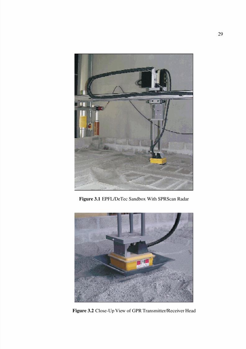
ratory consisted of a large sandbox as shown in Figure 3.1, approximately 3m x 3m, into

which either sand or soil could be placed. A close-up view of the GPR transmitter/receiver

head is shown in Figure 3.2.

7/29/2019 10.1.1.116.1392


29

Figure 3.1 EPFL/DeTec Sandbox With SPRScan Radar

Figure 3.2 Close-Up View of GPR Transmitter/Receiver Head

7/29/2019 10.1.1.116.1392


30

Each mine £le consists of 21 stacked B-scans taken at 2.0 cm intervals for a total

swath width of 42 cm. For the analysis presented here, only the £rst 20 B-scans are used.

Each B-scan consists of 98 A-scans, with each A-scan taken every 1.0 cm. The number of

signal samples for each A-scan is 512 with an effective sampling rate of 40 GHz. Thus the

time resolution for each A-scan is 25 picoseconds (ps), and the total time duration is 12.8

nanoseconds (ns). The layout of the grid is shown in Figure 3.3. The data here are from

either the x- or y- scan direction, given by the £le names on the following plots.

Figure 3.3 Scanning Pattern of DeTec Laboratory SPRScan Radar

3.1.1. Data Collected in Cambodia

The DeTec-1 system shown in Figure 3.4 was tested in Karlovac, Croatia, in July

1997, in a military £eld in which live mines had been planted the same morning.

7/29/2019 10.1.1.116.1392


31

Figure 3.4 DeTec-1 Handheld GPR In Croatia

7/29/2019 10.1.1.116.1392


32

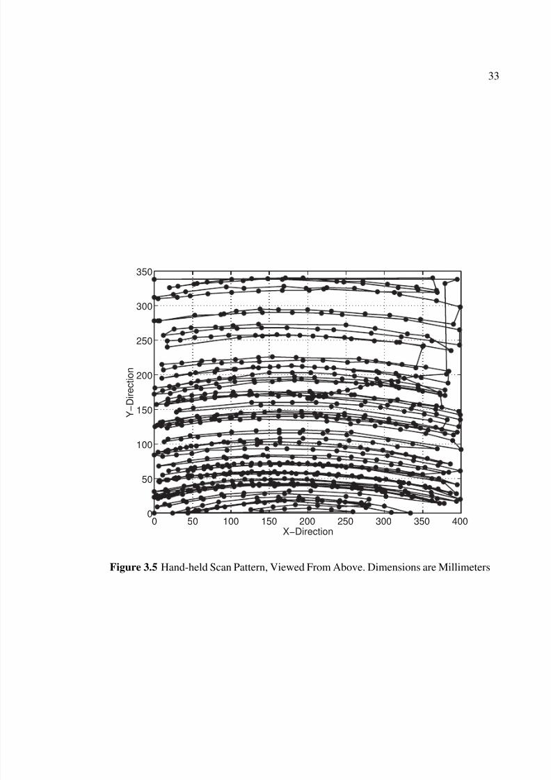
The test was quite instructive and demonstrated that the head of a hand-held device

must not weigh more than 1 Kg. In addition, it was determined that, for good data, the

mines must be buried in the ground several months prior to the tests; otherwise, the dis-

turbance around the mine creates a severe clutter environment. From Figure 3.5, it can be

seen that the hand-held antenna, used in the kneeling position, results in a rather erratic

scan pattern. The operator will tend to increase the distance between consecutive scans as

the antenna moves farther from the body, and the scans become clustered as the antenna

comes closer to the body. This results in uneven sampling of the target area and can create

problems in interpretation of data. An additional factor is that the operator tends to raise

the antenna off the ground slightly when a real mine possibly lies beneath the surface; the

variation in height also creates data anomalies. The particular antenna used in all these

tests (ERA Technologies, Ltd. SPR-Scan) was designed originally for civil engineering

applications and normally requires contact with the surface of the ground. The system

was redesigned with all equipment inside the same box, supporting a moving arm which

included a simple mechanism for doing the regular scanning, resulting in much improved

data quality.

Discussions between EPFL/DeTec and the non-governmental organization (NGO)

HALO Trust in Cambodia in November 1996 led to the design by EPFL of a hand-held

antenna to be used by a kneeling deminer (or in the prone position). In November 1997,

the author accompanied Prof. J.-D. Nicoud and F. Guerne to Cambodia to collect data with

the DeTec-2 hardware. A map of the test area is shown in Figure 3.6. The author was

also able to practice the current manual demining techniques with metal detector and prod

(Figure 3.7).

7/29/2019 10.1.1.116.1392


33

0 50 100 150 200 250 300 350 4000

50

100

150

200

250

300

350

Y −

D i r e c t i o n

X−Direction

Figure 3.5 Hand-held Scan Pattern, Viewed From Above. Dimensions are Millimeters

7/29/2019 10.1.1.116.1392


34

Figure 3.6 Location of Mine Fields, Thmar Pouk, Cambodia

Figure 3.7 Author Demining with Ebinger Metal Detector

7/29/2019 10.1.1.116.1392


35

DeTec-2 (http://diwww.epfl.ch/w3lami/detec/detec2.html ) suf-

fered some dif£culties the £rst day due to the 32 degree (90 degree F) weather, but these

problems were £xed by applying toothpaste to an aluminum plate which served as an ad-

ditional heat sink. From then on, the equipment could operate for about 2-3 hours, permit-

ting good data collection. The £rst day (18 November) was mostly devoted to equipment

set-up and check-out, solving our heat problems and explaining to the deminers how to

proceed; we collected only 4 £les. On the second day we conducted 7 hours of data ac-

quisition (22 £les). On the third day we collected 21 £les, including data from 4 mines.

The last half-day took place in the countryside (12 £les). In all, about 500MB of data were

collected; all the data are available at http://diwww.epfl.ch/w3lami/detec/

detec2cambodia.html. Power for recharging DeTec-2 was provided at the HALO

facility by an additional car battery connected to a 220V converter. HALO Trust had al-

located a team of 6 deminers to assist us during our tests. The chief of the platoon spoke

English quite well. One deminer was in charge of the equipment. Two pairs of deminers

conducted the removal of the vegetation, metal detection and prodding. Metal detector

alarms were indicated on the ground with wooden triangles, and DeTec-2 was then put in

position for the scanning. Positioning took 1-2 minutes, scanning 2-3 minutes. In opera-

tion, the normal SOP was followed by a deminer £rst scanning the ground with the metal

detector. When a suspected target was found, the deminer would report that to the DeTec-2

operator, who would then move into position within the demined lane and adjust the GPR

head position to be a few centimeters above the ground.

The local DeTec-2 disk had suf£cient capacity for 50 acquisitions, due to the high

spatial density of data points. This was enough for 4 days of operation. However, to ensure

that no data would be lost due to equipment malfunctions, it was copied onto a streamer

tape and also backed up on the author’s laptop PC every evening. Recharging the DeTec-2

7/29/2019 10.1.1.116.1392


36

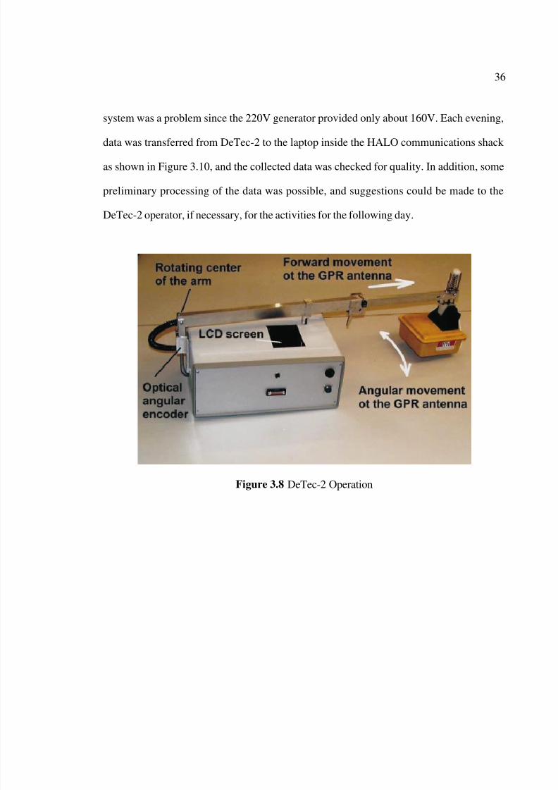
system was a problem since the 220V generator provided only about 160V. Each evening,

data was transferred from DeTec-2 to the laptop inside the HALO communications shack

as shown in Figure 3.10, and the collected data was checked for quality. In addition, some

preliminary processing of the data was possible, and suggestions could be made to the

DeTec-2 operator, if necessary, for the activities for the following day.

Figure 3.8 DeTec-2 Operation

7/29/2019 10.1.1.116.1392


37

0 100 200 300 4000

50

100

150

200

250

300

350

400

Figure 3.9 DeTec-2 Scan Pattern

Figure 3.10 Author’s Laptop, DeTec-2 in Background

7/29/2019 10.1.1.116.1392


38

3.2. Data Collected at the Vrije Universiteit Brussel (VUB)

In March and April 1999, the author participated in extensive GPR data collection

at the VUB with his colleague, Luc van Kempen, under the direction of the VUB Program

Manager, Prof. Hichem Sahli. This data collection effort was partially in support of the EU

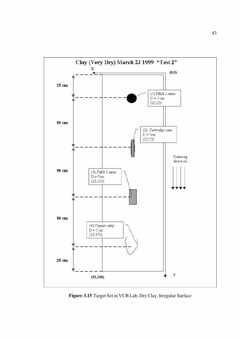
humanitarian demining program DEMINE. Figures 3.12 through 3.15 depict the target sets

for the tests. The equipment used was the identical DeTec laboratory equipment described

above. The objective of this series of tests was to extend the target sets to take advantage

of the lessons learned from the Cambodia collections, that is, include numerous interfering

objects such as roots, rocks and additional material which all can cause serious false alarms

with the GPR. In Cambodia, it was found that a realistic mine£eld environment includes

numerous targets which confuse both metal detectors and GPRs. For example, the metal

detector often alarmed when common £rebricks were encountered. In other cases, moist

roots and rocks appeared to the GPR to be probable mines. Therefore, in the VUB tests,

actual metal clutter and a rock taken from Cambodia were used as interfering targets.

The VUB laboratory setup included, in addition to an area containing sand, a test

area consisting only of a clayey soil. This soil also had an uneven surface to more closely

approximate real-world conditions. Finally, to provide additional realism, the soil was

soaked with water (Figure 3.11) and GPR measurements were made of the test area imme-

diately after the soaking and also after three weeks had passed to permit some drying of the

soil surface.

7/29/2019 10.1.1.116.1392


39

Figure 3.11 Author Soaking Clay in Preparation for Experiments

7/29/2019 10.1.1.116.1392


40

Figure 3.12 Target Set in VUB Lab, Dry Sand, Flat Surface; Multiple Objects to Present

Interfering Clutter

7/29/2019 10.1.1.116.1392


41

Figure 3.13 Target Set in VUB Lab, Dry Sand, Flat Surface

7/29/2019 10.1.1.116.1392


42

Figure 3.14 Target Set in VUB Lab, Wet Clay, Irregular Surface

7/29/2019 10.1.1.116.1392


43

Figure 3.15 Target Set in VUB Lab, Dry Clay, Irregular Surface

7/29/2019 10.1.1.116.1392


44

3.3. Data Collected at The Technische Universität Ilmenau

In March 1999 the author, while at the VUB, developed a test protocol for use at the

TUI lab. An objective of the test was to demonstrate the viability of a stepped frequency

GPR in contrast to the more standard pulse GPR. In theory, by stepping through a 6 GHz

bandwidth, one should be able to effectively synthesize an impulsive waveform and obtain

pulse-like data. In April 1999, the author participated in the data collection at TUI. Prof.

Jürgen Sachs of TUI directed the overall collection program under the auspices of the EU

DEMINE Program.

3.3.1. TUI Lab Setup and Scanning Method

The sandbox is approximately 2.2 m long and 0.75 m wide. This permits up to four

separate targets to be placed in such a manner to ensure at least 40 cm spacing between the

targets. The frame for mounting the antennas is attached to the ceiling of the laboratory.

Two carriages for the receive and transmit antennas may be moved independently in one

direction. The antennas are in a bistatic con£guration and may be rotated to obtain all

combinations of horizontal, vertical and cross-polarizations. The radar device at TUI is a

network analyzer to permit ¤exibility in measurements.

The data is collected by dwelling at a particular position in a grid and sweeping

from 0 to 6 GHz in 15 MHz steps, for a total of 401 frequency samples per A-scan. Figures

3.16 and 3.17 illustrate the principle. Compare to Figure 1.11 on page 23.

A typical test setup at TUI is shown in Figure 3.18. Each target was buried such

that the top of each was 5.0 cm below the surface of the sand.

7/29/2019 10.1.1.116.1392


45

0 1 2 3 4 5 6−120

−100

−80

−60

−40

−20

0

Frequency, GHz

M a g n i t u d e , d B

Figure 3.16 Magnitude Spectrum of Typical Scan at TUI

0 2 4 6 8 10 12−0.02

−0.015

−0.01

−0.005

0

0.005

0.01

0.015

Time, ns

A m p l i t u d e

Figure 3.17 Resultant A-scan, Time Domain

7/29/2019 10.1.1.116.1392


46

Figure 3.18 Measurement Scenario at TUI Lab

7/29/2019 10.1.1.116.1392


47

3.4. Data Collected at the Belgian Royal Military Academy (RMA)

The author was provided a CD containing wideband (10 GHz) pulse GPR data

which had been collected at the RMA in the Summer of 1999. Dr. Marc Acheroy and

Major Bart Scheers kindly provided the data which was collected using an experimental

antenna designed at RMA. The normalized transmitted pulse is shown in Figure 3.19.

0 0.5 1 1.5 2−1

−0.8

−0.6

−0.4

−0.2

0

0.2

0.4

0.6

0.8

1

Time, nsec

N o r m a l i z e d A m p l i t u d e

Figure 3.19 Transmitted Waveform of RMA GPR

7/29/2019 10.1.1.116.1392


CHAPTER 4

CLUTTER CHARACTERIZATION AND REMOVAL

Clutter removal is an important part of GPR signal processing; as shown in Figure

1.11, the target is literally swamped by the clutter environment. Therefore, some means

must be devised to remove as much clutter as possible while maintaining details about the

target. A common method is to simply compute the mean vector of a number of A-scans

and subtract this value from each A-scan. This method fails, however, if the contour of the

ground surface is not smooth. Therefore, clutter A-scan samples may be taken from areas

known to not contain targets, and those samples (or models thereof) may be subtracted

from individual A-scans. In this dissertation, characterization of clutter is accomplished

using system identi£cation methods.

4.1. Clutter Characterization

Clutter detected by the GPR includes many components: crosstalk from transmit-

ter to receiver antenna, initial ground re¤ection and background resulting from scatterers

within the soil. In this dissertation, all of these components are considered to be undesired

signals which require estimation and subsequent removal in order to enhance the target

signal. As mentioned previously, the target signal can be either a mine or non-mine; it is

the objective of the post-processing to make the decision between the two.

48

7/29/2019 10.1.1.116.1392


49

System Identi£cation methods [62] offer considerable promise in GPR signal pro-

cessing. One goal of system identi£cation is to attempt to determine a target impulse re-

sponse which will be invariant with aspect angle and soil conditions. In general, this will

not be possible [47]-[49],[63][64]. Aspect-invariant impulse responses, characterized by

the natural resonant poles of the system, are valid only when the target is perfectly con-

ducting and in free space.

4.1.1. The GPR Signal Model

Estimating the target parameters is the goal of system identi£cation applied to GPR

signal processing. If speci£c parameters of the target can be isolated in some domain, then

it may be possible to classify the target further into “Mine” and “Non-Mine” categories.

The roots of the transfer function polynomials may be plotted in either the z-domain or

the s-domain, and an appropriate distance function can be applied to separate the target

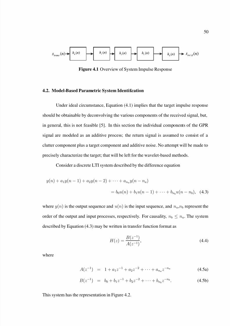
sets. Figure 4.1 shows the basic structure of the input-output relationship is between the

transmitted signal and the received signal. From this diagram,

srecd(n) = strans(n) ∗ ha(n) ∗ hc(n) ∗ ht(n) ∗ hc(n) ∗ ha(n), (4.1)

where ha(n),hc(n) and ht(n) are the impulse responses of the antenna, clutter and target,

respectively. The symbol ∗ denotes linear convolution, de£ned as

u(n) ∗ h(n) :=∞

k=−∞

h(k)u(n− k). (4.2)

The antenna and clutter impulse responses are shown twice to reinforce the fact that the

radar wave passes through both components twice. Strictly speaking, in a bistatic array

environment, the antenna impulse responses should be denoted harec(n) and hatrans(n) to

denote the receiver and transmitter antenna responses which will, in general, be different.

7/29/2019 10.1.1.116.1392


50

Figure 4.1 Overview of System Impulse Response

4.2. Model-Based Parametric System Identi£cation

Under ideal circumstance, Equation (4.1) implies that the target impulse response

should be obtainable by deconvolving the various components of the received signal, but,

in general, this is not feasible [5]. In this section the individual components of the GPR

signal are modeled as an additive process; the return signal is assumed to consist of a

clutter component plus a target component and additive noise. No attempt will be made to

precisely characterize the target; that will be left for the wavelet-based methods.

Consider a discrete LTI system described by the difference equation

y(n) + a1y(n− 1) + a2y(n− 2) + · · ·+ anay(n− na)

= b0u(n) + b1u(n − 1) + · · ·+ bnbu(n− nb), (4.3)

where y(n) is the output sequence and u(n) is the input sequence, and na,nb represent the

order of the output and input processes, respectively. For causality, nb ≤ na. The system

described by Equation (4.3) may be written in transfer function format as

H (z ) =B(z −1)

A(z −1), (4.4)

where

A(z −1) = 1 + a1z −1 + a2z −2 + · · · + anaz −na (4.5a)

B(z −1) = b0 + b1z −1 + b2z −2 +

· · ·+ bnbz −nb . (4.5b)

This system has the representation in Figure 4.2.

7/29/2019 10.1.1.116.1392


51

H z( )B z

1–( )

A z 1–( )

----------------=u n( ) y n( )

Figure 4.2 Discrete LTI Block Diagram

The more general case includes additional measurement noise e(n) which is as-

sumed to be independent identically distributed (i.i.d.) with mean zero. In this case, the

input-output relation is written

A(z −1)y(n) = B(z −1)u(n) + e(n), (4.6)

which is the equation-error in system identi£cation language [62]. De£ne the parameter

vector θ as

θ =

a1, a2, . . . ana, b0, b1, . . . bnb

T , (4.7)

and the elements of this vector are the parameters to be estimated. Let

x(k) =

−y(k − 1), . . . ,−y(k − na), u(k), . . . , u(k − nb)

T

then

y(k) = xT (k)θ + e(k) (4.8)

or

y = X θ + e, (4.9)

where X is the matrix

X =

xT (n + 1)

xT (n + 2)

...

xT

(n + N )

=

−y(na), . . . , −y(1), u(nb + 1), . . . , u(1)

−y(na + 1), . . . , −y(2), u(nb + 2), . . . , u(2)

.... . .

.... . .

−y(na + N − 1), . . . , −y(N ), u(nb + N ), . . . , u(N )

,

(4.10)

7/29/2019 10.1.1.116.1392


52

where N is the length of a sliding data window; N na + nb. Hsia [65] shows that the

solution of Equation (4.9) is given by the minimum-norm

θ = (X T X )−1X T y = X †y, (4.11)

where X † is the Moore-Penrose Pseudo-inverse [66] of X .

Figure 4.3 is a general block diagram of the three main components of the received

signal. Estimated parameters may be used for feature extraction and clutter-reduction;

an example of clutter features which result from parameter estimation using the Steiglitz-

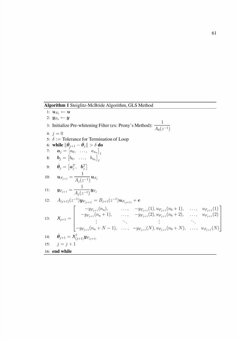
McBride algorithm, Algorithm 1 on page 61.

H ˆ c z( )Bˆ z

1–( )

Aˆ z1–

( )

----------------=

H ˆ

t z( )Dˆ z

1–( )

C ˆ z1–

( )-----------------=

⊕

H ˆ

νz( )

F ˆ z1–

( )

G z 1–( )

-----------------=

e n( )

δ n( )

n( )

sc

n( )

ν n( )

st

n( )

⊕

+

+

+

+

-

y n( )

r n( ) y n( )

Figure 4.3 General Block Diagram Representation of System Identi£cation

7/29/2019 10.1.1.116.1392


53

4.2.1. The Target Model

The target model is shown in Figure 4.4. The impulse response of the target is ht(n),

and the input-output relationship is as shown, with a Dirac δ -function as the input, and the

output sequence by st(n). As stated previously, the goal will be to estimate the parameters

of the transfer function, D(n) and C (n) given by the composite parameter vector

θt = [c1, c2, . . . , cnc, d0, d1, . . . , dnd]T , (4.12)

where nc,nd represent the order of the respective polynomials in z −1.

H

ˆ

t z( )

Dˆ z1–

( )

C ˆ z1–( )

-----------------=

δ n( )

st

n( )

Figure 4.4 Representation of Target Parametric Model

The parameters of the target may be estimated only after the clutter/antenna param-

eters are determined.

4.2.2. The Clutter Model

In a similar way, the clutter model is represented by Figure 4.5 as

θc = [a1, a2, . . . , ana, b0, b1, . . . , bnb]T . (4.13)

7/29/2019 10.1.1.116.1392


54

The input to the clutter block diagram is indicated by the δ -function in the absence

of any knowledge of the true input waveform. In this way, the clutter model includes all of

the effects noted in Section 4.1 on page 48. In general, the shape of the transmitted pulse

will not be known. Indeed, as with the data collected at TUI, there is no “pulse” per se,

but only a synthesized pulse by virtue of the stepped frequency modulation. The modeling

methods described in this section, however, lend themselves equally well to the case where

the input (transmitted) pulse is known; simply replace the δ -function with the known pulse.

H ˆ c z( )Bˆ z

1–( )

Aˆ z1–

( )

----------------=δ n( ) sc

n( )

Figure 4.5 Representation of Clutter Parametric Model

4.2.3. The Noise Model

When modeling dynamical systems or signals, it is usually necessary to include a

noise model which will account for any random disturbances caused by the measurement

equipment, etc. Such disturbances may be non-stationary, and may also be non-Gaussian

and display some speci£c spectral characteristics other than a ¤at (“white”) spectrum. The

inclusion of a (possibly time-varying) noise model is therefore indicated.

Such a noise process model can be described by

θν =

g1, g2, . . . , gng , f 0, f 1, . . . , f nf T

, (4.14)

and the model is shown in Figure 4.6.

The input to the noise model is a vector of (i.i.d.) samples with a Gaussian amplitude

7/29/2019 10.1.1.116.1392


55

distribution of zero mean and constant spectral intensity. The input is applied to a £lter

which will provide appropriate spectral and amplitude shaping to represent the measured

noise from A-scan to A-scan; it may not be necessary to apply this £lter if the noise from

A-scan to A-scan is suf£ciently decorrelated.

H ˆ ν z( )F ˆ z

1–( )

Gˆ z1–

( )

-----------------=

e n( )

ν n( )

Figure 4.6 Representation of Added Noise Parametric Model

For a general description of the parametric system identi£cation algorithms de-

scribed in this dissertation, reference is made to Figure 4.3 and the additional £gures im-

mediately following. The clutter model is estimated by applying the Steiglitz-McBride

Algorithm to a measured clutter sample with a Dirac δ -function as the input, as in Figure

4.5. The clutter model is derived from a reference clutter sample, as is the case in all the

techniques described here except for some types of recursive (adaptive) methods which will

be described in Section 4.2.4. This should not, in most cases, be a drawback to the general

method; representative clutter samples may be collected at various times during the mine

scanning process.

7/29/2019 10.1.1.116.1392


56

The noise model shown in Figure 4.6 is estimated by determining the ARMA pa-

rameters of the residue found by subtracting successive A-scans and then using those co-

ef£cients to create correlated noise samples ν (n) which are of appropriate amplitude to

match the power of the original residue. It has been experimentally determined that, with

the data samples of interest here, the noise transfer function may be omitted; in other words,

the scan-to-scan noise is closely approximated by the input e(n). If an examination of the

correlation properties of the differenced A-scans determines that the residue had signi£cant

correlations at lags much greater than zero, it would be necessary to determine the noise

model ARMA parameters as, for example, described by Swami and Mendel [67]. That ref-

erence uses higher-order statistics (cumulants) to determine ARMA parameters assuming

the data is correlated and possibly non-Gaussian. Other ARMA estimation methods may

be used, such as those in Ljung [62] if the process is found to be linear and Gaussian. In

practice, it was found that WGN was a close approximation to the true process; in no case

was an ARMA model greater than ARMA(4,4) determined to be of use.

An example of the ef£cacy of the model-based approach, Figures 4.7 and 4.8 show

the before and after B-scans of a cylindrical copper plate buried 30 cm in sand. The un-

cancelled clutter in Figure 4.8 may be due to undulations in the sand surface. As noted

previously, this method is non-adaptive in this example, but the basic model may be re£ned

to include adaptivity in which case such surface clutter may be reduced.

Once the clutter estimate and noise processes are determined, the target model may

be extracted by simply subtracting the sum of those estimates from the measured signal.

If desired, the target £lter coef£cients may be easily determined by the Steiglitz-McBride

algorithm applied to the new target estimate signal as for the clutter signal described above.

7/29/2019 10.1.1.116.1392


57

Distance, cm

T i m e , n s e c

0 40 80 120 160 200

0

1

2

3

4

5

Figure 4.7 B-scan of Copper Plate Buried 30cm in Sand

Distance, cm

T i m e , n s e c

0 40 80 120 160 200

0

1

2

3

4

5

6

7

8

Copper Plate

Figure 4.8 Result of Model-Based Clutter Removal

7/29/2019 10.1.1.116.1392


58

4.2.4. Recursive (Time-Varying) Methods

Recursive algorithms, also known as adaptive algorithms [62],[68] are used for

on-line processing of data as opposed to batch or off-line processing. In the case of clutter-

reduction, two approaches are addressed in this dissertation: the case where a sample of

clutter is available for estimation, and the case where there is no a priori clutter information.

In either case, the ultimate goal is to determine the parameter vector θt given by Equation

(4.12).

Consider

y(n) = xT (n)θ(n) + e(n). (4.15)

The general expression for recursive parameter estimation is

θ(n) = θ(n− 1) + k (n) (y(n) − y(n)) , (4.16)

where k (n) is the adaptation gain vector . Given an initial parameter vector

θ0(n) = θ0(n− 1) + w(n), (4.17)

where w(n) is assumed to be i.i.d. The general algorithm for recursive parameter estima-

tion is

θ(n) = θ(n− 1) + k (n) [y(n) − y(n)] (4.18a)

y(n) = xT (n)θ(n− 1) (4.18b)

k (n) = Q (n)x(n) (4.18c)

Q (n) =P (n− 1)

R2 + xT (n)P (n− 1)x(n)(4.18d)

P (n) = P (n− 1) − P (n− 1)x(n)xT

(n)P T

(n− 1)R2 + xT (n)P (n− 1)x(n)

+ R 1, (4.18e)

7/29/2019 10.1.1.116.1392


59

where R 1 = E [w(n)wT (n)] and R2 is the variance of the innovations in Equation (4.15),

R2 = E [e2(n)]. This is the Kalman Filter version of adaptive parameter identi£cation.

The covariance matrix P is typically initialized as a diagonal matrix of dimension N ×N ,

where N = na + nb as in Equation (4.3), for example.

Often, a modi£cation to the above equations is made to include a forgetting factor

{λ : 0 < λ ≤ 1}, in which case Equations (4.18d) and (4.18e) become, respectively,

Q (n) =P (n

−1)

λ + xT (n)P (n− 1)x(n) (4.19a)

P (n) =

P (n− 1) − P (n− 1)x(n)xT (n)P T (n− 1)

λ + xT (n)P (n− 1)x(n)

λ. (4.19b)

Typical values for λ range from 0.95 to 0.99.

7/29/2019 10.1.1.116.1392


60

4.3. Implementation and Algorithm

The clutter model is £rst estimated using the Steiglitz-McBride algorithm, which is

a generalized least-squares (GLS) solution to the output-error model

sc(n) = y(n) =B(z −1)

A(z −1)δ (n) + e(n), (4.20)

where e(n) is an i.i.d process representing modeling errors. This equation can be repre-

sented as

A(z −1)y(n) = B(z −1)δ (n) + A(z −1)e(n), (4.21)

which is almost, but not exactly, of the same form as Equation (4.6); the noise process

is now no longer i.i.d., but is effectively £ltered by A(z −1). The iterative algorithm to

accomplish the calculation of B(z −1) and A(z −1) follows [65]:

7/29/2019 10.1.1.116.1392


61

Algorithm 1 Steiglitz-McBride Algorithm, GLS Method

1: uF 0 ← u

2: yF 0 ← y3: Initialize Pre-whitening Filter (ex: Prony’s Method):

1

A0(z −1)4: j = 05: δ := Tolerance for Termination of Loop

6: while θ j+1 − θ j > δ do

7: a j =

a0, . . . , ana

j

8: b j =

b0, . . . , bnb j

9: θ j =

aT j , bT j

10: uF j+1 =

1

A j(z −1)uF j

11: yF j+1 =1

A j(z −1)yF j

12: A( j+1)(z −1)yF (j+1)= B j+1(z −1)uF (j+1)

+ e

13: X j+1 =

−yF j+1(na), . . . , −yF j+1

(1), uF j+1(nb + 1), . . . , uF j+1

(1)−yF j+1(na + 1), . . . , −yF j+1(2), uF j+1(nb + 2), . . . , uF j+1(2)

.... . .

.... . .

−yF j+1(na + N − 1), . . . , −yF j+1(N ), uF j+1(nb + N ), . . . , uF j+1(N )

14: θ j+1 = X

†

( j+1)yF (j+1)

15: j = j + 1

16: end while

7/29/2019 10.1.1.116.1392


CHAPTER 5

WAVELET-BASED TARGET FEATURE DETECTION

This chapter describes the application of the wavelet transform to removing noise

from a signal and the relationship between the wavelet transform and the regularity of a

function. The wavelet transform is used in two different contexts in this dissertation. In

the £rst, wavelet packet based noise reduction is employed to remove much of the residual

noise which is present following clutter-reduction. The wavelet packet method is selected

because of a unique property of wavelets in general and wavelet packets in particular;

namely, the ability to remove only speci£c portions of a signal in different frequency bands

without disturbing adjacent bands.

The second property of wavelets which is exploited here is the relationship between

the regularity of a function (the “smoothness” of the function) and the wavelet transform.

It will be shown that the detail coef£cients of the wavelet transform can be used to localize

singularities in a function. The application here is direct: the GPR signal phase undergoes

an abrupt change at the interface between two media such as the soil and the target, and the

wavelet transform coef£cients are used to locate that interface.

62

7/29/2019 10.1.1.116.1392


63

5.1. The Wavelet Transform

The wavelet transform is a speci£c type of time-frequency distribution [69]-[89] and

is characterized by the ability to segment the time-frequency plane into localized regions

of interest.

Consider the Fourier transform of a piecewise-continuous function f (t) ∈ L2(R),

F (ω) = +∞

−∞

f (t)e−iωtdt. (5.1)

The complex kernel e−iωt represents an in£nite collection of sinusoids which are in£nite

in time extent; thus, the ability of the Fourier transform to determine the local spectral

behavior of a function is limited by the fact that the observation interval is in£nite. Figure

5.1a shows the tiling with the Fourier basis; because of the in£nite extent of the exponential

kernel (“in£nite support”), the Fourier transform is unable to show any local frequency

content.

The Gabor transform [69] and the Short-Time Fourier Transform (STFT) are exten-

sions of the standard Fourier transform with a “window” function multiplying the kernel,

thus providing a measure of localization. Figure 5.1b is an example of the STFT tiling.

The Continuous Wavelet Transform (CWT) of a function f (t) ∈ L2(R) replaces the

sinusoidal kernel of the Fourier transform with a scale and shift kernel|a|

−1/2

ψ t−b

a ,

(Wψf ) (b, a) = |a|−1/2 +∞−∞

f (t)ψ

t − b

a

dt = f, ψ, (5.2)

where ψ is a wavelet . Properties of wavelets are summarized below. Figure 5.1c shows the

tiling of the time-frequency (scale) plane by the wavelet kernel.

7/29/2019 10.1.1.116.1392


64

0 0.5 10

0.2

0.4

0.6

0.8

1Fourier Basis Tiling

Time(a)

F r e q u e n c y

0 0.5 10

0.2

0.4

0.6

0.8

1Gabor Basis Tiling

Time(b)

F r e q u e n c y

0 0.5 10

0.2

0.4

0.6

0.8

1 Wavelet Basis Tiling

Time(c)

F r e q u e n c y

0 0.5 10

0.2

0.4

0.6

0.8

1 Wavelet Packet Tiling

Time(d)

F r e q u e n c y

Figure 5.1 Tilings of the Time-Frequency (Time-Scale) Plane

7/29/2019 10.1.1.116.1392


65

5.1.1. Wavelet Properties

The analysis in this chapter is based upon the existence of a (dyadic) scaling func-

tion ϕ, a corresponding orthogonal wavelet function ψ, corresponding sequences {ak},

{bk}, { pk}, {q k} in 2, and a corresponding set of approximation subspaces {V j : j ∈ Z}

which satisfy all of the following:

• Subspace Relationships.

{ϕ(t

−k)

}is an orthogonal basis for V 0 and

· · · ⊂ V −1 ⊂ V 0 ⊂ V 1 ⊂ · · · ⊂ L2(R) (5.3)

closL2

j∈Z

V j

= L2(R) (5.4)

j∈Z

V j = {0}. (5.5)

• Function Decomposition

f (t) ∈ V j ⇔ f (2t) ∈ V j+1, (5.6a)

f (t) ∈ V j ⇔ f

t +

1

2 j

∈ V j. (5.6b)

• Dilation Equation

ϕ(t) =

k pkϕ(2t− k). (5.7)

• Decomposition Relationship

ϕ(2 j+1t− l) =k

a2k−lϕ(2 jt − k) + b2k−lψ(2 jt− l)

. (5.8)

• Two-Scale (Reconstruction) Relationship

ϕ(2 jt) =

k pkϕ(2 j+1t− k), (5.9a)

ψ(2 jt) =k

q kϕ(2 j+1t− k). (5.9b)

7/29/2019 10.1.1.116.1392


66

For example, the Daubeschies wavelet Db4 scaling function coef£cients are given

by

p0 =1 +

√ 3

4, p1 =

3 +√

3

4, p2 =

3 −√ 34

, p3 =1−√ 3

4, pk = 0 otherwise,

(5.10)

so for j = 0 in Equations (5.9a) and (5.9b),

ϕDb4(t) =3

k=0

pkϕ(2t − k) (5.11a)

ψDb4(t) =1

k=−2

(−1)k p1−kϕ(2t− k) (5.11b)

= p3ϕ(2t + 2) − p2ϕ(2t + 1) + p1ϕ(2t)− p0ϕ(2t − 1). (5.11c)

The sequence { pk}, associated with a given orthonormal wavelet such as Db4, uniquely

de£nes the remaining sequences because

q k = (−1)k p1−k (5.12a)

ak =1

2 pk (5.12b)

bk =1

2(−1)k p1−k. (5.12c)

For each integer j, W j denotes the corresponding wavelet (detail) subspace de£ned

as the orthogonal complement of V j in V j+1 using the L2 inner product,

f, g =

∞−∞

f (t)g(t)dt. (5.13)

Each approximation subspace is then the direct sum of the smaller approximation subspace

and the corresponding detail subspace,

V j+1 = V j ⊕ W j

= V j−1 ⊕ W j−1 ⊕ W j

= · · · .

(5.14)

7/29/2019 10.1.1.116.1392


67

Each approximation subspace V j, as well as L2(R), can be represented as a direct sum of

mutually orthogonal detail subspaces,

V j =k<j

W k = · · · ⊕ W j−2 ⊕ W j−1 (5.15)

and

L2(R) = j∈Z

W j = · · · ⊕ W −1 ⊕W 0 ⊕ W 1 · · · . (5.16)

For each j, k∈Z, de£ne

ψ j,k = 2 j/2ψ(2 jt− k). (5.17)

Chui [73] shows that each ψ j,k is in W j and that the entire set of these functions forms an

orthogonal basis for L2(R). That is, for any g ∈ L2, the function g is represented by the

series

g(t) = j,k∈Z

dk

j ψ j,k(t) (5.18)

with

dk j = g, ψ j,k = (Wψg)

k

2 j,

1

2 j

, (5.19)

where (Wψf ) (b, a) is given by Equation (5.2).

Equation (5.18) is analogous to the representation of a signal as a Fourier series,

with the exponential kernel bring replaced by the wavelet ψ j,k(t). Equation (5.19) shows

that the wavelet series coef£cients {ck j} are given by the continuous wavelet transform

evaluated at the dyadic points (b, a) =

k2j

, 12j

with j, k ∈ Z.

5.1.2. Wavelet Deconposition of Discrete Signals

The preceding lays the foundation for wavelet decomposition of functions in L2(R).

For signal processing applications, discrete signals are used, represented by N -dimensional

samples. Thus L2(R) is identi£ed with RN . The function subspaces V j and W j are now

7/29/2019 10.1.1.116.1392


68

identi£ed with the linear subspaces in RN (also denoted V j and W j) generated by sampling

the functions in the original function subspaces. The received signal is then an approxima-

tion, and an appropriate scaling function ϕ and sample size N may be chosen (generally,

N is chosen to be an integer power of 2) so that every sampled function (signal) may be

assumed to be in V 0.

Let f be a function. By assumption f ∈ V 0. From the preceding section, the signal

may be represented by the following direct sum of orthogonal subspaces,

V 0 = W −1 ⊕ V −1 (5.20)

= · · · ⊕ W −1 ⊕ · · · ⊕ W −M ⊕ V −M (5.21)

with N = 2M . Therefore f may be written as the direct sum of the components with

respect to these subspaces,

f (t) = g−1(t) + g−2(t) + · · ·+ g−M (t) + f −M (t), (5.22)

where, for each j ∈ Z,

g j(t) ∈ W j (5.23)

and

f j(t) ∈ V j. (5.24)

The approximation component f j at the j-th scale is generated by the scaling function

f j(t) =k

ck j ϕ(2 jt− k), (5.25)

and the detail component of the function at the j-th scale is generated by the wavelet

g j(t) =k

dk j ψ(2 jt− k). (5.26)

Figure 5.2 depicts the decomposition of the received signal into approximation and detail

subspaces.

7/29/2019 10.1.1.116.1392


69

V 0

©

d

d d

d d

d d

d V −1 W −1

©

d d

d

V −2 W −2© d d

V −3 W −3

Figure 5.2 Signal Subspace Decomposition Diagram

The sequences {ck j} and {dk j} are the scaling function and wavelet coef£cients, re-

spectively. It is seen that the components of the received signal vector y (the sampling of

f ) is simply the sequence {ck0} ≡ c0.

The above shows that a signal can be decomposed into low-pass and high-pass com-

ponents using the wavelet and scaling functions. It is shown next that the decomposition

can be accomplished without having to rely explicitly on the wavelet or scaling function.

Recall that, for orthogonal wavelets, V j+1 = V j ⊕W j. If a discrete signal is represented by

the N -dimensional real vector c0, wavelet decomposition to the next scale results in new

sequences {ck−1} and {dk−1}.

From Equation (5.22),

f j+1 = f j + g j. (5.27)

7/29/2019 10.1.1.116.1392


70

For the orthonormal scaling function ϕ,

f j+1(t) =k

ck j+1ϕ(2 j+1t− k), (5.28a)

f j(t) =k

ck j ϕ(2 jt− k), (5.28b)

and

g j(t) =k

dk j ψ(2 jt− k). (5.29)

The objective of the decomposition algorithm is to obtain

{ck j}

and

{dk j

}from

{ck j+1

},

f j+1(t) =l

cl j+1ϕ(2 j+1t− l)

=l

cl j+1

k

a2k−lϕ(2 jt− k) + b2k−lψ(2 jt − k)

=k

ckj l

a2k−lcl j+1

ϕ(2 jt− k)

f j(t)

+k

dkj l

b2k−lcl j+1

ψ(2 jt− k)

gj(t)

.

(5.30)

Thus, the {ck j} and {dk j} may be obtained from {ck j+1} as follows:

ck j =l

a2k−lcl j+1 (5.31a)

dk j =

l

b2k−lcl j+1. (5.31b)

Similarly, the reconstruction of a function from the approximation and detail coef£-

cients can be accomplished without direct use of the wavelet or scaling function. Applying

the two-scale relationships of Equation (5.9),

f j(t) + g j(t) =l

cl jϕ(2 jt− l) +l

dl jψ(2 jt − l)

=l

cl jk

pkϕ(2 j+1t− 2l − k) +l

dl j

k

q kϕ(2 j+1t− 2l − k)

= k

ckj+1

l

pk−2lcl

jl

q k−2ldl

jϕ(2 j+1

t− k) f j+1(t)

,

(5.32)

7/29/2019 10.1.1.116.1392


71

from which the {ck j+1} may be obtained

ck j+1 =l

pk−2lcl j +

l

q k−2lcl j. (5.33)

5.2. Quadrature Mirror Filters

In practice, the discrete wavelet transform is implemented with quadrature mirror

£lters (QMF), with decomposition (analysis) £lters H 0 and H 1, and reconstruction (synthe-

sis) £lters F 0 and F 1. The construction of these £lters is described by Strang and Nguyen

[77]. The basic relationship between the £lters is shown in Equation set (5.34). The build-

ing block is the £lter F 0, which is simply the scaling function coef£cient sequence { pk}

of the selected wavelet. Figure 5.3 is a symbolic representation of the formation of the

low-frequency wavelet coef£cients c0 j and the high frequency wavelet coef£cients d0 j ; the

superscript is used here for consistency with the discussion of wavelet packets in Section

5.3. The downsampling symbol ↓ 2 denotes that every other sample from the £lter is used.

F 0(z ) = −H 1(z ) (5.34a)

F 1(z ) = H 0(−z ) (5.34b)

H 1(z ) =

−H 0(

−z −1)z −N (5.34c)

c0 j ← (c0 j+1)↓2H 0 =⇒ (c0 j+1) E H 0 E ↓ 2 Ec0 j

d1 j ← (c0 j+1)↓2H 1 =⇒ (c0 j+1) E H 1 E ↓ 2 Ed1

j

Figure 5.3 Symbolic Representation of Wavelet Coef£cient Decomposition

7/29/2019 10.1.1.116.1392


72

5.3. Wavelet Packets

It was shown in Section 5.1.1 that the scaling function and wavelet function gen-

erated mutually orthogonal sets of subspaces V j and W j, respectively, as shown in Figure

5.2. This decomposition of a signal results in high-frequency components de£ned by g j and

low-frequency components de£ned by f j. However, it is possible to further decompose the

high-frequency components in a manner similar to the original signal wavelet decompo-

sition. Such a further decomposition results in a £ner resolution in the scale (frequency)

plane, and is accomplished by wavelet packets. Wavelet packets generate sets of mutually

orthogonal subspaces within each W j. In order to accommodate the added complexity of

representation, denote any orthogonal subspace by U n j , where the subscript j ∈ Z identi£es

the scale of the decomposition and the superscript {n : n = 0, . . . , 2| j| − 1, n ∈ Z} is

an index within a scale, as shown in Figure 5.4. The subspaces with even index are gener-

ated by the scaling function and the subspaces with odd index are generated by the wavelet

function. Thus,

U n j+1 = U 2n j ⊕ U 2n+1 j . (5.35)

The wavelet packet functions µn j , n = 2l or 2l + 1, l = 0, 1, . . . , are now de£ned by

µ2n j (t) =

k pkµn

j+1(2t − k)

µ2n+1 j (t) =

k

q kµn j+1(2t− k).

(5.36)

These functions are derived from the scaling function ϕ and wavelet function ψ by de£ning

µ0−1(t) := ϕ(t)

µ1−1(t) := ψ(t).

(5.37)

Thus, the subspaces U with even index are generated by wavelet packets µ2n derived from

the scaling function ϕ, and the subspaces with odd index are generated by wavelet packets

µ2n+1 derived from the wavelet function ψ.

7/29/2019 10.1.1.116.1392


73

U 00

©

H 0

d d

d d

d d

d d

H 1

U 0−1 U 1−1

©

H 0 d d

d

H 1

©

H 0 d d

d

H 1

U 0−2 U

1−2 U

2−2 U

3−2

© H 0

d d H 1

© H 0

d d H 1

© H 0

d d H 1

© H 0

d d H 1

U 0−3 U 1−3 U 2−3 U 3−3 U 4−3 U 5−3 U 6−3 U 7−3

Figure 5.4 Wavelet Packet Subspace Decomposition Diagram, Including QMF

7/29/2019 10.1.1.116.1392


74

Figure 5.5 is a schematic of the process of wavelet decomposition of any node un j

to the next level, represented by the nodes u2n+1 j−1 and u2n

j−1, through the action of downsam-

pling the outputs of the quadrature mirror £lters H 1 and H 0, respectively. The reconstruc-

tion of the coef£cients at level j is denoted by un j and is accomplished by upsampling the

approximation and detail coef£cients and subsequent £ltering by F 1 and F 0, respectively.

Figure 5.6 is a symbolic representation of the decomposition into wavelet and wavelet

packet coef£cients which is used for the algorithms in Section 5.5 on page 81.

un j

E H 1 E ↓ 2 Eu2n+1 j−1

E ↑ 2 E F 1 Eun j

~ &

& &

& &

& & b

H 0 E ↓ 2 Eu2n j−1

E ↑ 2 E F 0

Figure 5.5 Two-Channel QMF For Perfect Reconstruction

c0 j ← (c0 j+1)↓2H 0 =⇒ (c0 j+1) E H 0 E ↓ 2 Ec0 j

d1 j ← (c0 j+1)↓2H 1 =⇒ (c0 j+1) E H 1 E ↓ 2 Ed1

j

u2n j ← (un

j+1)↓2H 0 =⇒ (un j+1) E H 0 E ↓ 2 Eu2n

j

u2n+1 j ← (un

j+1)↓2H 1 =⇒ (un j+1) E H 1 E ↓ 2 Eu2n+1

j

Figure 5.6 Symbolic Representation of Wavelet Packet Coef£cient Decomposition

The ability of wavelet packets to decompose the time-scale plane into £ner divisions

than the wavelet transform is demonstrated in Figures 5.7 and 5.8; it is seen that the wavelet

packet decomposition allows an adaptive tiling of the time-scale plane.

7/29/2019 10.1.1.116.1392


75

0

0.1

0.2

0.3

0.4

0.5

0.6

0.7

0.8

0.9

1

−14−12−10−8−6−4−20Entropy

N o r

m a l i z e d F r e q u e n c y ( S c a l e )

U−1

1

U−1

0

U−2

1

U−2

0

U−3

3

U−3

0

U−3

1

Figure 5.7 Wavelet Packet Best Basis Entropy Tree, Chirp Signal

Time

N o r m a l i z e d F r e

q u e n c y ( S c a l e )

0 0.1 0.2 0.3 0.4 0.5 0.6 0.7 0.8 0.9 10

0.1

0.2

0.3

0.4

0.5

0.6

0.7

Figure 5.8 Wavelet Packet Tiling of Time-Scale Plane

7/29/2019 10.1.1.116.1392


76

5.3.1. De-Noising Using Wavelet Packet Entropy-Based Best Bases

As stated previously, any irregularities in the soil will cause the GPR return to ap-

pear noisy, and it is necessary to remove some of that interference in order to improve sig-

nal detectability. The term “de-noising” is rather ambiguous and overused; it is, in general,

impossible to recover a desired signal embedded in noise. While most signal processing

texts consider noise to be additive, wideband (“white”) and with amplitude distributed as

a Gaussian distribution, real measured data do not necessarily exhibit these characteristics.

On the other hand, one may speak in terms of degrees of noise removal based on certain

criteria.

The usual noise reduction method employs simple £ltering with no regard given

to the recovery of the original signal, except in a mean-square sense. Filtering (usually,

high-pass £ltering) can remove desired high-frequency components of the signal while

leaving “noise” in the lower frequency bands. Wavelet packets provide a unique method

of selectively removing “just enough” noise throughout the signal bandwidth. As shown

in Figures 5.4 and 5.7, the partitioning of the signal subspaces may be adaptively thresh-

olded to remove “noise” while at the same time retaining signal features. Donoho [90]

provides speci£c criteria for evaluating the performance of a “de-noising” strategy; specif-

ically, the smoothness of the resultant signal and the adaptivity of the thresholding process

are detailed.

The concept of a “Best Basis” [12] involves searching an ordered set of orthogonal

(orthonormal) basis coef£cients and deciding which coef£cients may be removed while

simultaneously maintaining as much information content in the signal as practical. Such

approaches are used in signal compression and de-noising, for example. As used here,

each A-scan signal will be decomposed into a library of wavelet packet bases, and speci£c

7/29/2019 10.1.1.116.1392


77

thresholds based on the entropy of the signal will be applied to decide which coef£cients

will be removed. It is shown in Reference [12] that the wavelet packet tree as depicted

in Figure 5.4 constitutes a library of wavelet packet bases. In addition, an algorithm is

developed which “prunes” the packet tree in accordance with the entropy or information

measure contained within each branch of the tree. Coifman and Wickerhauser [12] de£ne

the entropy at node j, n from Figure 5.4 as

vn j = − p

n j , ln p

n j , (5.38)

where

pn j =

|un j,1|2, |un

j,2|2, . . . ,un

j, N

2|j|

2

, (5.39)

where un j,k denotes the kth wavelet packet coef£cient in node j, n.

The Best Basis at a given node will depend on the entropy of the two nodes at the

next lower level, the “children” nodes. If the entropy of a parent node is less than the sum

of entropy measures of the two children, then the Best Basis is the parent node, and the

two children nodes are removed; the basis tree is “pruned.” If the entropy of the parent is

greater than the sum of the entropy of the two children, then the Best Basis is simply the

two children, and the tree is not “pruned” at those nodes.

5.3.2. De-Noising by Thresholding the Wavelet Packet Coef£cients

Following the construction of the Best Basis tree, an entropy-based threshold may

be applied to the tree nodes to remove noisy coef£cients. The selection of an appropriate

threshold is suggested by Donoho [90] in consideration of the following property [91]: Let

{z} be an i.i.d. random sequence over N (0, 1) (Gaussian distribution with zero mean, unity

variance, then

P rz∞ ≤ √ 2 ln n

→ 1, n →∞, (5.40)

7/29/2019 10.1.1.116.1392


78

where n is the length of the vector z. Thus, a simple threshold of

√ 2 ln n

may be applied to the basis tree nodes following Best Basis selection.

5.4. Singularity Detection Using Wavelets

Mallat and Hwang [92] derive the properties of wavelets which de£ne their ability

to locate discontinuities in functions. These properties will be used here to locate the edges

of the APL’s by exploiting the fact that, at each mine interface, a phase reversal of the

transmitted pulse takes place. One way the “smoothness” of a function can be expressed

is in terms of its Lipschitz exponent α (also Hölder exponent), which is a representation

of how closely the function can be approximated by a polynomial; a function is said to be

“singular” if it exponent is not Lipschitz 1. Formally,

De£nition 5.1. Let α ∈ R, n ∈ Z+, n ≤ α ≤ (n + 1). A function f (t) is said to

be Lipschitz α (also Hölder exponent α) at some point t0, if and only if there exist two

constants A and h0 > 0, and a polynomial P n of order n such that for |h| < h0,

|f (t0 + h)− P n(h)| ≤ A|h|α. (5.41)

Furthermore,

(i) The function f (t) is uniformly Lipschitz α over the interval (a, b) if and only if there

exists a constant A and for any t0 ∈ (a, b) there exists a polynomial P n(h) of order n

such that Equation (5.41) is satis£ed if t0 + h ∈ (a, b).

(ii) A function f is singular at t0 if it is not Lipschitz 1.

For the application here, the goal is to assess the singularity of a function at a point ,

not in some interval. The ability to do so, while at the same time relaxing the requirement

7/29/2019 10.1.1.116.1392


79

for continuous differentiability of the wavelet ψ(t) was treated by Jafard [93], who estab-

lished the following theorem which requires only that the wavelet function ψ(t) have n

vanishing moments, is n-times continuously differentiable and has compact support.

Theorem 5.1 (Regularity at a Point). 1. Let n ∈ Z+ and α < n. Let f (t) ∈ L2(R). If

f (t) is Lipschitz α at t0 , then there exists a constant A such that for all points t in the

neighborhood of t0 and any scale j

| (Wψf ) (t, j)| ≤ A( jα + |t − t0|α). (5.42)

2. Assume α is not an integer. Then the function f (t) is Lipschitz α at t0 if the following

two conditions apply:

(a) There exists some > 0 and a constant A such that for every point t in a

neighborhood of t0 and any scale j

| (Wψf ) (t, j)| ≤ Aj. (5.43)

(b) There exists a constant B such that for every point t in a neighborhood of t0

and any scale j

| (Wψf ) (t, j)| ≤ B| j|α +

|t− t0|α

|log

|t−

t0||

. (5.44)

Theorem 5.1 proves that the wavelet transform is well-suited to provide a measure

of singularities in a function. Mallat and Hwang [92] prove that local singularities in a

function may be determined by the wavelet modulus maxima at small details, and the Lips-

chitz exponent may be estimated if needed. This property is illustrated in Figure 5.9 which

shows the localization of the singularities in the signal by the wavelet transform.

7/29/2019 10.1.1.116.1392


80

Time

S c a l e

0 0.1 0.2 0.3 0.4 0.5 0.6 0.7 0.8 0.9 1

2

3

4

5

6

7

8

9

0 0.1 0.2 0.3 0.4 0.5 0.6 0.7 0.8 0.9 1−6

−4

−2

0

2

4

6

Figure 5.9 Wavelet Modulus Maxima (Bottom) of a Discontinuous Signal (Top)

7/29/2019 10.1.1.116.1392


81

5.5. Detailed Listing of Algorithms

The algorithms in this section, written in MATLAB-style pseudocode, are a com-

pilation of the theoretical foundations of the preceding two chapters. Figure 5.10 summa-

rizes the methodology established in the preceding chapters.

7/29/2019 10.1.1.116.1392


82

APPLY CLUTTERREMOVAL PROCEDURE

LOAD A-SCANSData Format Must BeSpecified e.g., SEG,ASCII, etc.

WAVELET PACKET-

BASED NOISEREDUCTION

ALGORITHMS 2 TO 6

RECONSTRUCT WPCOEFFICIENTS TO

FINEST DETAIL (LEVEL 1)ALGORITHM 7

MODEL-BASED USINGALGORITHM 1

ADAPTIVE (RLS)METHOD

STACK RECONSTRUCTEDDETAILS INTO B-SCAN

END

Figure 5.10 Program Flow

7/29/2019 10.1.1.116.1392


83

Algorithm 2 Create Wavelet Packet Decomposition

Require: Choose H 01: m = dim(y)2: J = log2(m)3: W (:, 1) = yT → c00 ∈ V 0 {W is Wavelet Packet Table}

4: for j = 1 : 1 : J do

5: for n = 0 : 1 : (2 j − 1) do

6: c0 j

←(c0 j−1)↓2H 0

7: d1 j ← (c0 j−1)↓2H 1

8: un j ← (u

n2 j−1)↓2H 0, n even

9: un j ← (u

n−12

j−1 )↓2H 1, n odd

10: W

1:

m

2 j, j + 1

= c0 j

11: W

m

2 j+ 1:

m

2 j−1, j + 1

= d1

j

12: W

nm

2 j+ 1:

(n + 1)m

2 j, j + 1

= un

j

13: end for

14: end for

Algorithm 3 Create Entropy Basis Tree

1:for j = 0 : J do2: for n = 0 : (2 j − 1) do

3: p =

W

nm

2 j+ 1:

(n + 1)m

2 j, j + 1

2

c00224: B(2 j + n) = −( p ln( p)) {B is Entropy at Node 2 j + n}

5: end for

6: end for

7/29/2019 10.1.1.116.1392


84

Algorithm 4 Select Best Entropy Basis1: A← B

2: for j = J − 1 : −1 : 0 do

3: for n = 0 : 2 j − 1 do

4: if B(2 j + n) < B(2 j+1 + 2n) + B(2 j+1 + 2n + 1) then

5: A(2 j + n) = B(2 j + n)6: A(2 j + n) = 0 {A is Best Basis Flag}

7: else

8: A(2 j + n) = B(2 j+1 + 2n) + B(2 j+1 + 2n + 1)9: A(2 j + n) = 1

10: end if 11: end for

12: end for

Algorithm 5 Prune Entropy Basis Tree

1: for j = 0 : 1 : J do

2: for n = 0 : 1 : 2 j − 1 do

3: if A(2 j + n) == 0 then

4: Γ = 2ln(mJ ) {Threshold Applied to Coef£cients}

5: ρ ← |u jn| − Γ6: ρ ← ρ + ρ/27: u jn| ← Sign(ρu jn)

8: u2n j+1 ← 0 {Succeeding Child Nodes Set to Zero}

9: u2n+1 j+1 ← 0

10: else

11: un j ← un

j

12: end if

13: end for14: end for

Algorithm 6 Threshold and Reconstruct Signal

1: for j = J : −1 : 1 do

2: for n = 0 : 2 : 2 j do

3: vn2 j−1 = (un

j )↑2F 0 + (un+1 j )↑2F 1 {Reconstruct by Upsampling and Filtering}

4: end for

5: end for

7/29/2019 10.1.1.116.1392


CHAPTER 6

RESULTS

This chapter summarizes the results of the clutter-reduction and wavelet-based edge

extraction techniques described in the preceding chapters.

6.1. Results of Clutter-Reduction Techniques

This section describes the results of applying both common mean background re-

moval and adaptive (RLS) background removal as described in Chapter 4. These methods

have been applied to all sources of data used here, but the TUI data is summarized because

a quantitative analysis of the performance measures was applied to this data at VUB. The

laboratory setup for the TUI data is described in Section 3.3.

6.1.1. Model Estimated Background Removal

Figure 6.1 shows the result of the clutter and noise estimation described in Section

4.1.1. In this £gure, the far right side has been removed to eliminate the re¤ections from

the wall of the sandbox. It is seen that the correlated clutter represented normally by waves

below the targets, is suppressed. In this way, the dominant returns are only the tops of

the targets. The reduction in correlated clutter is achieved by decorrelating the clutter by

the addition of colored ARMA noise. The noise model was estimated by differencing

85

7/29/2019 10.1.1.116.1392


86

consecutive A-scans and evaluating the autocorrelation properties in order to establish the

ARMA model order. Then, WGN was applied to the noise process transfer function shown

in Figure 4.6. The clutter process was estimated by applying the Dirac delta function to

the clutter transfer function of Figure 4.5 and experimentally determining the appropriate

order by using a clutter A-scan sample. In Figure 6.1 the clutter parameters were £xed, but

the noise parameters were updated from A-scan to A-scan.

Distance, cm.

T i m e , n a n o s e c .

0 20 40 60 80 100 120 140 160

0

0.5

1

1.5

2

2.5

3

3.5

4

4.5

5

PMA−3 Sphere Rock

Figure 6.1 Parametric Model Background Removal

7/29/2019 10.1.1.116.1392


87

6.1.2. RLS Background Removal

Figure 6.2 shows the results of the RLS adaptive approach. In this case, the clutter

parameters are again considered £xed, but the signal minus clutter residue is adaptively

estimated in time (depth) as well as from A-scan to A-scan. In this £gure, the sphere

and rock returns are reduced, but the level of correlated clutter is more than the previous

approach.

Distance, cm

T i m e , n a n o s e c .

50 100 150 200

0

0.5

1

1.5

2

2.5

3

3.5

4

4.5

5

PMA−3 Sphere Rock PMA−1

Figure 6.2 RLS Background Removal

7/29/2019 10.1.1.116.1392


88

6.2. Performance Measures of Clutter-Reduction Methods

As stated in Section 1.5.1, SNR or SCR are not considered to be valid measures

of performance (MOP) in GPR evaluation. 1 Rather, evaluate GPR MOP in the context

of improvement in, for example, target classi£cation. In the following section, physical

target parameters and target discrimination performance are evaluated following adaptive

background removal by the RLS method.

6.2.1. Physical Parameter Estimation

An important parameter in the processing of GPR data is the knowledge of the ve-

locity of propagation in the medium. The velocity estimation is based on the detected hy-

perbolas in the vertical B-scan image. In the following the estimated hyperbolic parameters

and velocities are compared for both GPR raw data (after simple average subtraction) and

following clutter-reduction using the techniques described in Chapter 4. The detection of

target hyperbolas in the B-scans was accomplished by using a generalized Hough-transform

on the detected edge pixels. Edge detection was performed using Gaussian and multi-scale

Gabor £lters, the details of which are in Brooks et al. [5] The following equation for the

general hyperbolic parameters was used:

t2 = α + β (x − γ )2, (6.1)

where t and x represent the vertical and horizontal coordinates. Figures 6.3 and 6.4 show

the detected hyperbolas for the raw data before and after adaptive clutter background re-

moval.

1This section is summarized in Brooks et al. [5] and the feature classi£cation analysis was performed by

Luc van Kempen of the VUB.

7/29/2019 10.1.1.116.1392


89

Figure 6.3 Detected Hyperbolas in Mean-Removed Background

Figure 6.4 Detected Hyperbolas RLS-Removed Background

7/29/2019 10.1.1.116.1392


90

In both cases a number of hyperbolas are detected at each of the object positions.

There are, however, additional hyperbolas which are present and do not correspond to real

objects. For each object the local velocity of propagation can be determined by

v =2∆x√

β ∆t(6.2)

and the depth

z = v√

α, (6.3)

where ∆x is the horizontal distance between two sample points (the horizontal scanning

step), ∆t is the difference in time between two sample points (the inverse of the sampling

frequency). Table 6.1 compares velocity, depth and eccentricity for the data before and

after adaptive clutter background removal.

Table 6.1 Feature Comparison between Mean-Removed and RLS-Processed Data

Raw Data Processed Data

Depth Velocity Eccentricity Depth Velocity Eccentricity

PMA-3 4.7 cm 5.7e+7 m/s 20.5 5.6 cm 6.9e+7 m/s 19.8

Sphere 6.5 cm 6.4e+7 m/s 21.0 6.1 cm 7.1e+7 m/s 19.9

Rock 4.9 cm 6.7e+7 m/s 20.8 6.4 cm 6.5e+7 m/s 19.1

PMA-1 8.1 cm 7.0e+7 m/s 23.1 5.6 cm 7.2e+7 m/s 19.8

It is seen that, with the RLS-processed data, the estimated depth is approximately

5cm for the mines, which is close to the correct value, and the velocity estimates for the

mines are approximately identical. Finally, the eccentricity is almost identical for all the

objects.

7/29/2019 10.1.1.116.1392


91

This latter observation, the similarity of hyperbolic eccentricities for all targets,

actually mitigates against using hyperbolic parameters for target discrimination. It is clear

that selecting classi£cation features based upon these parameters will not lead to ef£cient

class discrimination.

6.2.2. Target Class Discrimination

Table 6.2 shows the comparison results, based on the de£ned values, for time, fre-

quency and wavelet features separately, or when using all (combined) features. The clus-

tering within the class is for the three objects (mine, sphere and rock) in most of the cases

better in the RLS-processed data than in the raw data. Finally the classes are better sepa-

rated using the RLS-processed data.

Table 6.2 Comparison Results Based on Feature Selection

Raw Data Pre-processed Data

Clustering (λ1/λ2) Separability Clustering (λ1/λ2) Separability

Mine Sphere Rock Mine Sphere Rock

Time 1.45 3.96 3.06 5.76 1.06 4.29 1.23 8.14

Freq 3.33 3.19 2.83 4.47 1.99 2.74 2.67 3.31

Wavl 3.21 2.65 1.38 2.77 2.82 2.68 2.49 4.23

All 16.42 21.52 4.46 1.19 2.17 1.67 2.67 6.85

7/29/2019 10.1.1.116.1392


92

6.3. Results of Wavelet-Based Target Discrimination

The following subsections summarize the results of the wavelet-based de-noising

and edge detection techniques described in Chapter 5. It is shown that details of the mine

targets are emphasized while simultaneously reducing the shape features of false targets.

This is also shown to be a function of the GPR pulse bandwidth, with improved results

at the wider instantaneous bandwidth of 10 GHz. An important result of this effort has

been the determination that the wavelet-based techniques are not effective with the swept-

frequency data collected at TUI. The probable reason is that the frequency swept scanning

technique required a signi£cant dwell time at each grid point to permit all 401 frequencies

to be sampled. This has the effect of averaging the GPR return over each A-scan, thus

destroying the details of the target edges.

6.3.1. 2 GHz Pulse Data From EPFL/DeTec Laboratory

The data collected at the EPFL/DeTec laboratory provided the basis for the prelimi-

nary experiments with the wavelet-based approaches described above. Due to the relatively

narrow bandwidth, the results are somewhat inconclusive. Figure 6.5 shows a typical B-

scan of a PMN buried 5 cm in sand, and Figure 6.6 shows the result of application of the

Best Basis detection method; the mine is faintly discernible, but there is no other target

which can be used for comparison of the method.

7/29/2019 10.1.1.116.1392


93

Scan Length, cm

T

i m e , n s

y

0 20 40 60 80

1

2

Figure 6.5 PMN Mine, RLS Clutter Removal

7/29/2019 10.1.1.116.1392


94

Scan Length, cm

T

i m e , n s

0 20 40 60 80

1

2

3

Figure 6.6 PMN Mine, Wavelet-Detected

7/29/2019 10.1.1.116.1392


95

6.3.2. 2 GHz Pulse Data from Cambodia

The data is of suf£cient quality for analysis. This is due to the small scan (40

cm square) over which the data was collected. Also, the high water content of the soils

contributed to poor detection with the existing low-power equipment.

6.3.3. 2 GHz Pulse Data From VUB Laboratory

The experiments conducted by the author and VUB personnel in the Spring of 1999

were explicitly designed to include numerous additional targets in the soil and sand in order

to achieve a more reliable method of comparing processing approaches. The experience in

Cambodia served a very useful purpose in that it made clear the need to collect data which

includes several target types. The Cambodia effort also established the need for a minimum

spacing of about 50cm between targets in the laboratory in order to ensure good visibility

between interfering target hyperbolas. This practice was also extended to the experiments

conducted at TUI.

Figures 6.7 through 6.9 show the evolution in processing the rock and mine targets

£rst shown in Figure 1.10 on page 21. It is apparent that the Best Basis approach results in

a suppression of the rock return, based on the irregular shape of the rock. This is apparent

even at the relatively narrow bandwidth of the ERA GPR.

7/29/2019 10.1.1.116.1392


96

Scan Length, cm

T

i m e , n s

0 40 80 120 160 200 240

1

2

3

4

5

6

RockMine

Surface Clutter

Figure 6.7 Rock and Mine

7/29/2019 10.1.1.116.1392


97

Scan Length, cm

T

i m e , n s

0 40 80 120 160 200 240

1

2

3

4

5

6

Rock

Mine

Figure 6.8 Rock and Mine, Clutter Removed

7/29/2019 10.1.1.116.1392


98

Scan Length, cm

T

i m e , n s

0 40 80 120 160 200 240

1

2

3

4

5

6

PMA−3 MineRock

Surface Clutter

Figure 6.9 Best Basis Approach, Showing Suppression of False Target (Rock)

7/29/2019 10.1.1.116.1392


99

6.3.4. 6 GHz Data from TUI

As stated previously, the results from applying the Best Basis approach to the

frequency-stepped GPR data collected at TUI were inconclusive. Figure 6.10 shows the

results of applying the Best Basis approach to the data shown in Figure 6.2 on page 87.

The mines show up well, and the re¤ections from the wall are suppressed, but there is no

clear de£nition of the mine features.

Scan Length, cm.

T i m e , n s

File f3049004

0 40 80 120 160 200

0.5

1

1.5

2

2.5

3

3.5

4

4.5

PMA−3Sphere

Rock

PMA−1

Figure 6.10 Best Basis Results With TUI Frequency-Stepped GPR

7/29/2019 10.1.1.116.1392


100

6.3.5. 10 GHz Pulse Data From RMA

The 10GHz data from RMA re¤ects the bene£t of a very wide bandwidth pulse, but

the data is limited in that there are only either mines or rocks in the data sets, none appear

simultaneously. So, only relative performance of the Best Basis approach can be assessed

at this time, but the results appear very promising.

Figures 6.11 through 6.14 show comparisons between the background-removed tar-

gets and the same targets detected with the Best Basis approach. Figure 6.14 dramatically

shows the suppression of the stone when the Best Basis approach is applied.

Finally, Figures 6.15 and 6.16 show a slice of a 3-D image of the mine and stone

created by visualizing the 3-D scanned volume. The stone is simply missing. Residual

surface clutter appears in both £gures.

7/29/2019 10.1.1.116.1392


101

0

10

20

30

40

50 0

10

20

30

40

50

−1

−0.5

0

0.5

1

Scan Length, cm

File pmn_2_s, Time Slice 1.17 ns.

Scan Length, cm

Figure 6.11 PMN Mine C-scan, Clutter Removed

0

10

20

30

40

50 0

10

20

30

40

50

−1

−0.5

0

0.5

1

Scan Length, cm

File pmn_2_s, Time Slice 1.17 ns.

Scan Length, cm

Figure 6.12 Best Basis Detected PMN Mine

7/29/2019 10.1.1.116.1392


102

0

10

20

30

40

50 0

10

20

30

40

50

−1

−0.5

0

0.5

1

Scan Length, cm

File st_2_s, Time Slice 1.12 ns.

Scan Length, cm

Figure 6.13 Stone, Clutter Removed

0

10

20

30

40

50 0

10

20

30

40

50

−1

−0.5

0

0.5

1

Scan Length, cm

File st_2_s, Time Slice 1.12 ns.

Scan Length, cm

Figure 6.14 Best Basis Detected Stone

7/29/2019 10.1.1.116.1392


103

Figure 6.15 PMN Mine Volume, Side View

Figure 6.16 Stone Volume, Side View

7/29/2019 10.1.1.116.1392


CHAPTER 7

SUMMARY OF CONTRIBUTIONS AND

SUGGESTIONS FOR FURTHER RESEARCH

The broad objective of this research was to develop new and innovative signal

processing techniques to improve the detectability of buried anti-personnel land mines

(APL’s) using ground penetrating radar (GPR). Using contemporary techniques, common

non-lethal objects such as rocks and roots often appear as lethal targets, thus considerably

slowing-down the discrimination/identi£cation process. The present research has resulted

in the incorporation of very promising wavelet-based algorithms for GPR signal processing

which have demonstrated the ability to suppress false targets while simultaneously enhanc-

ing shape features of the APL. These results were obtained with realistic targets using real,

measured data rather than computer simulations.

7.1. Speci£c Contributions of This Dissertation

The research results presented in this dissertation have contributed to the £eld of

humanitarian demining technology in the following ways:

• In work conducted on-site with the VUB/EU DEMINE Project, the author enhanced

their GPR laboratory measurement program using realistic mine and non-mine (clut-

ter) targets. The data collected are available to the demining research community.

104

7/29/2019 10.1.1.116.1392


105

• With the support from VUB, the author developed novel, adaptive clutter-reduction

algorithms for GPR, based on system identi£cation methods, which are demonstrably

superior to standard clutter-reduction approaches previously used.

• The author independently developed wavelet-based algorithms for GPR detection of

APL’s which suppress signals associated with non-mine objects while simultaneously

enhancing shape features of buried APL’s. These wavelet-based algorithms have

been shown to be applicable to wide-band pulse GPR modulation. This achievement

represents a signi£cant contribution to the £eld of humanitarian demining technolo-

gies because it advances the GPR technique beyond the realm of “blob detector.”

7.2. Suggestions for Further Research

The humanitarian demining technologies in use today remain quite crude, with the

common metal detector and basic, manual prodding used almost universally. Clearly, a

metal detector is ineffective with non-metallic APL’s, so the operator is still constrained

to manually prod for such mines. The research presented in this dissertation has advanced

the effectiveness of GPR techniques for APL detection, but much additional research is

needed to investigate the bounds of these wavelet-based algorithms and develop improved

versions.

The thresholding method described here is rather simple. Improved thresholding

algorithms should be investigated to exploit particular wavelet properties.

The sensitivity of the GPR algorithms developed here, to various wavelet families,

should be investigated by considering, for example, “spline wavelets.”

The wavelet-based algorithms developed here show promise when applied to raw

GPR data which has not been pre-processed for clutter removal. This feature has only

recently been discovered by the author, and additional investigations should be conducted.

7/29/2019 10.1.1.116.1392


106

The wavelet-based techniques for GPR signal processing, as considered here, are

not consistently effective with respect to arbitrary GPR modulations. As mentioned in

Chapter 6, the stepped-frequency modulation did not lend itself to application of the wavelet

techniques. This observation suggests the need for development of wideband pulse systems

vs. stepped-frequency systems if wavelet techniques are to be used. Additional research

should be conducted to determine the limits of applicability of the wavelet-based tech-

niques, and to re£ne those techniques for other modulation types.

The wave-like appearance of the target superimposed on the clutter, as shown in

Figure 1.11 on page 23 suggests the possible application of the “waveform-structure” mod-

eling and identi£cation technique associated with Johnson’s Disturbance-Accommodation

Control (DAC) Theory [94]-[97] in GPR clutter removal. In principle, the target may be

viewed as an uncertain “disturbance” within the dominant clutter signal, and a dynami-

cal “state-model” of that disturbance could be derived which may enhance the ability to

uniquely identify the target.

7/29/2019 10.1.1.116.1392


APPENDIX A

SOME TYPICAL ANTI-PERSONNEL LAND MINES

The mine types tested for this dissertation were the T-72, PMN-series, PMA-series

plastic mines. In addition, wooden box mines were encountered in Cambodia, but not

tested in a laboratory environment.

There are hundreds of different types of APL which have been manufactured by

over 50 countries [98]. The most insidious, and most dif£cult to detect, are the so-called

“minimum-metal” mines which are currently found in areas of more recent con¤ict: An-

gola, Afghanistan, Cambodia, Bosnia, etc. [2]. A particularly insidious APL is the Chinese

Type 72 shown in Figure A.1, which contains only about 74 grams of high explosive, known

in military parlance as a “toe-popper”. After the safety ring is removed, the only metallic

content in the mine is a £ring pin about the size of a small thumbtack; the spring mecha-

nism is made of plastic/composite materials. The Type 72 APL has seen widespread use

in Afghanistan, Cambodia, Kuwait, and increasingly throughout Africa. The green color

is characteristic of other Chinese plastic devices. While not expected to be widely encoun-

tered, there are two antidisturbance variants of the Type 72. The Type 72B shown in Figure

A.2 (diagram from a sales brochure) utilizes a ball-in-cage mechanism to function solely

as a boobytrap device. The Type 72B is intended to function both as an antipersonnel mine

and a boobytrap device. There have been reports that the Type 72B is very sensitive and can

107

7/29/2019 10.1.1.116.1392


108

be detonated in the presence of magnetic mine detectors. The South African Non-Metallic

APL, indigenously produced, is a direct copy of the Chinese Type 72 [99].

Figure A.1 Chinese Type 72 APL

Figure A.2 Details of T72B, Anti-

Handling Mechanism, from

Sales Brochure

7/29/2019 10.1.1.116.1392


109

For the TUI measurements, four different mine types were used: the Yugoslav

PMA-1, PMA-2 and PMA-3, and the Belgian PRB. During the £rst series of measure-

ments at TUI, the full complement of mines was used. However, the large horn antenna

provided by the UK Defense Research Establishment (DERA) resulted in unacceptable lev-

els of antenna ringing, so a subset of the measurements was conducted with a new ¤at-plate

“vivaldi” design. Because of this, and the limited time available for a full analysis, only the

PMA-1 and PMA-3 mines were used. These were selected because they were £lled with

RTV silicone and the PMA-1, being rectangular, provided a good prototype for that shape.

The detonators of each mine had been removed, as well as the explosive material.

In place of the explosive, RTV-1000 silicone rubber was placed, which has electrical prop-

erties very close to those of TNT.

The PMA-1 (Figures A.3 and A.4) is a plastic version of a box or “shu” mine with

a two-piece case. The lower section is a rectangular plastic box that houses the main TNT

charge and the MUV-type fuze (either UPM-1, Model 43, or UANU-1) and detonator unit.

The lid section is hinged to the lower box at one end and is designed to close over the lower

box. In the armed position, the lid rests on a striker retaining pin at the end of the fuze.

When pressure is applied, the lid removes the pin, beginning the initiation process. Probing

for small “shu” type mines with low pressure thresholds is a very hazardous operation.

7/29/2019 10.1.1.116.1392


110

Figure A.3 Exterior Dimensions of PMA-1

Figure A.4 PMA-1 Mines in Bosnia; Opened for View

7/29/2019 10.1.1.116.1392


111

The PMA-2 (Figures A.5 and A.6) is a relatively small antipersonnel mine with a

cylindrical body and a top-mounted UPMAH-2 chemical action pressure fuze. The sur-

face area of the UPMAH-2, which is exposed to pressure, is limited to a small pressure

spider with six legs. As a result, the PMA-2 is considered hardened or blast resistant.

The UPMAH-2 pressure fuze begins the £ring train, which consists of a detonator (con-

taining 2.55 grams of potassium chlorate, lead azide, antimony, and sul£de), a Hexogen

booster, and a TNT main explosive charge. The sole metallic content in the PMA-2 mine

and UPMAH-2 fuze is an aluminum disk (8.6 mm in diameter and 0.05 mm in thickness).

The assembly’s small size and extremely small metallic content results in a mine that is

extremely dif£cult to detect.

7/29/2019 10.1.1.116.1392


112


Figure A.6 Internal View of PMA-2

7/29/2019 10.1.1.116.1392


113

The PMA-3 (Figures A.7 and A.8) is a small APL, which consists of a ¤at cylindri-

cal body and the base-mounted UPMAH-3 chemical action pressure fuze. The PMA-3 is

designed to function only when the upper pressure plate rotates within the lower assembly

containing the UPMAH-3 fuze. The emplacement directions recommend a protective cover

of from 2.0 to 4.0 cm and horizontal placement of the pressure plate to take advantage of

the pressure hardened or blast resistant design. Additionally, the design for a non-axial

load means that the necessary pressure to function the mine decreases as the load is placed

closer to the edge. The normal pressure necessary to function the mine is described as a

range of from 8.0 to 20.0 Kg. However, it is possible that, when applied at the very edge, as

little as 3 Kg could function the mine. The UPMAH-3 pressure fuze with chemical friction

ignitor (containing potassium chlorate, red phosphorus and binder, and glass) begins the

£ring train which consists of an M-17 P2 detonator (containing tetryl, lead azide, and lead

styphnate), and a pressed TNT main explosive charge. The sole metallic content in the

PMA-3 mine and UPMAH-3 fuze is the aluminum covering on the M-17 P2 detonator cap.

This minimal metallic content renders the PMA-3 rather dif£cult to detect.

7/29/2019 10.1.1.116.1392


114


Figure A.8 Internal View of PMA-3

7/29/2019 10.1.1.116.1392


115

Other proli£c APL’s which are dif£cult to detect are the (former) Soviet PMN-types

and wooden mines [98]. Internal details of a PMN APL are shown in Figure A.9. It is a

delay-armed, pressure-£red, high explosive (blast) APL. The mine may be black, green,

or brown. The black and green mines have no markings. Markings may be found on the

bottom side of the brown mine. The mine case is plastic; the pressure plate cover is rubber.

The standard £ring assembly adapter plug and the SVP arming device are plastic. The PMN

weighs 454 grams, and contains about 200 grams of high explosive (HE) [98]. An example

of the Yugoslav PMU-style minimum-metal APL is shown in Figure A.11; a representative

box-mine is shown in Figure A.12.

7/29/2019 10.1.1.116.1392


116

Figure A.9 Russian PMN-Type APL

Figure A.10 PMN Details

7/29/2019 10.1.1.116.1392


117

Figure A.11 Yugoslav PMU Series MineFigure A.12 Example of Wooden Box

Mine

7/29/2019 10.1.1.116.1392


118

Several US-produced APL are commonly found in various post-con¤ict areas. Prob-

ably the most dif£cult to detect is the M14, Figures A.13 and A.14. The M14 and Ml4E1

are nonmetallic, pressure-initiated, blast, antipersonnel HE land mines which use an in-

tegral fuze with a steel £ring pin. The M14 series mines are olive drab with identifying

markings embossed in black on the bottom. The indicating arrow on the pressure plate and

the letters “A” and the “S” are yellow. The mine body, fuze body, and pressure plate are

plastic. The pressure plate must be rotated from the safe position to the armed position or

the plate cannot apply pressure to the belleville spring. The integral belleville spring fuze

and the safety features are contained in the upper portion of the mine. The mine weighs 85

grams, and the lower portion contains 29 grams of tetryl. The only metal in the mine is the

steel striker tip. Direct copies are produced in India (M-14) and Vietnam (MN-79), and a

similar mine is also produced by Vietnam (MD 82B) [99].

7/29/2019 10.1.1.116.1392


119

Figure A.13 U.S. M-14 APL

Figure A.14 U.S. M-14 APL, Details

7/29/2019 10.1.1.116.1392


120

REFERENCES

[1] “Basic fact sheet, UN demining data base,” 1998, http://www.un.org/Depts/

dha/mct/facts.htm.

[2] Bureau of Political-Military Affairs, “Hidden killers,” U.S. Dep’t of State Publica-

tion 10575, September 1998, http://www.state.gov/www/global/arms/

rpt\_9809\_demine\_toc.html .

[3] Eric Newsom, “On-the-record brie£ng on Hidden Killers report on humanitarian de-

mining,” Tech. Rep., September 1998.

[4] Ilaria Bottiglero, 120 Million Landmines Deployed Worldwide: Fact or Fiction?, Pen

& Sword Books, Ltd., London, U.K., 200.

[5] John W. Brooks, Luc van Kempen, and Hichem Sahli, “Ground penetrating radar data

processing: Clutter characterization and removal,” Tech. Rep. IRIS-TR-0059, Vrije

Universiteit Brussel, November 1999.

[6] Jean-Daniel Nicoud, “Mine clearance: Not only a problem for the military anymore,”

Proc. ISMCR’96, Brussels, BE,9-11 May, pp. 6–10, 1996.

[7] B.S.G. Janzen, “Improving the technology for humanitarian demining,” Proc. 1996

IEE/EUREL Conf. on the Detection of Hidden Land Mines, Edinburgh, UK, 7-9 Oct ,

pp. 11–15, 1996.

[8] K. Eblagh, “Practical problems in demining and their solutions,” Proc. 1996 IEE/EUREL

Conf. on the Detection of Hidden Land Mines, Edinburgh, UK, 7-9 Oct , pp. 1–5, Oc-

tober 1996.

[9] Maude Storme, “Microwave characterization of wet soils,” Tech. Rep. HuDEM

F97-06-WG1, Université Catholique de Louvain, April 1998.

[10] D. J. Daniels, Surface-Penetrating Radar , IEE Radar, Sonar, Navigation and Avionics

Series, Short Run Press, Ltd., Exeter, UK, 1996.

[11] Hollis C. Chen, Theory of Electromagnetic Waves, A Coordinate-Free Approach,

McGraw-Hill, New York, 1983.

[12] R. R. Coifman and M. V. Wickerhauser, “Entropy-based algorithms for best basis

selection,” IEEE Trans. Info. Theory, vol. 38, no. 2, pp. 713–718, February 1992.

[13] John Curtis, “Dielectric properties of soils,” Tech. Rep., Joint UXO Coorrdination

Offoce, September 1998.

7/29/2019 10.1.1.116.1392


121

[14] U. S. Army, “UXO technology demonstration program at Jefferson Proving Ground,

phase III,” Tech. Rep., U.S. Army Environmental Center Project Number SFIM-

AEC-ET-CR-9701, April 1997.

[15] A. J. Healey and W. T. Webberm, “Sensors for the detection of land-based munitions,”

Tech. Rep. Report NPS-ME-95-003, US Naval Postgraduate School, Monterey, CA,

USA, September 1995.

[16] Carl W. Helstrom, Statistical Theory of Signal Detection, Pergamon Press, second

edition, 1968.

[17] Fawwaz T. Ulaby, Richard K. Moore, and Adian K. Fung, Microwave Remote Sens-

ing, vol. II, Artech House, 1982.

[18] Christopher T. Allen, Kun Shi, and Richard G. Plumb, “The use of ground-penetrating

radar with a cooperative target,” IEEE Trans. Geoscience and Remote Sensing, vol.

36, no. 5, pp. 1821–1825, September 1998.

[19] Günter Wichmann, “Research and development on the £eld of mine detection, DTIC

No. ADA 325260,” Tech. Rep., European Research Of£ce of the U.S. Army, October

1996.

[20] S. L. Earp, E. S. Hughes, and T. J. Elkins, “Ultra-wideband ground-penetrating radar

for the detection of buried metallic mines,” EEE AES Systems Magazine, pp. 30–34,September 1996.

[21] L. Peters Jr., J.J. Daniels, and U. D. Young, “Ground penetrating radar as a subsurface

environmental sensing tool„” Proc. IEEE , vol. 82, December 1994.

[22] C. Bruschini, B. Gros, F. Guerne, P-Y Pièce, and O. Carmona, “Ground penetrating

radar and induction coil sensor imaging for antipersonnel mines detection,” Proc. 6th

Int’l Conf. on Ground Penetrating Radar , pp. 211–216, September 1996.

[23] E. Pettingelli, S.E. Beaubien, F. S. Marzano, and N. Pierdicca, “Comparison of GPR

£eld results from a strati£ed limestone terrain with model simulations,” Proc. 1995 Int’l Symposium on Geoscience and Remote Sensing, IGARSS 95, vol. 3, pp. 1705–

1707, 1995.

[24] A. J. Patterson, J. M. Tealby, and N. M. Allison, “Ground penetrating radar migration

with uncertain parameters,” Proc. 1995 Int’l Symposium on Geoscience and Remote

Sensing, IGARSS 95, pp. 27–29, 1995.

[25] A. J. Witten, J. A. Molyneaux, and J. E. Nyquist, “Ground penetrating radar tomog-

raphy: Algorithms and case studies,” IEEE Trans. Geoscience and Remote Sensing,

vol. 3, no. 2, pp. 461–467, March 1994.

7/29/2019 10.1.1.116.1392


122

[26] C. Bruschini and B. Gros, “A survey of current sensor technology research for the

detection of landmines,” SusDem’97, Zagreb (Croatia), 29 Sept.-1 Oct. 1997 , pp.

6.18–6.27, 1997.

[27] Ph. Maechler, “Detection technologies for anti-personnel mines,” Symposium on

Autonomous Vehicles in Mine Countermeasures, Monterey, CA, pp. 6.150–6.154,

1995.

[28] B. Gros and C. Bruschini, “Sensor technologies for the detection of antipersonnel

mines. a survey of current research and system developments,” ISMCR’96, Bruxelles,

pp. 564–569, May 1996.

[29] J. W. Brooks, “A survey of modern signal processing methods and their applicationto sustainable humanitarian demining,” Proc. Int’l Workshop on Sustainable Human-

itarian Demining, SusDem ´ S97 , pp. S5.41–S5.49, September 1997.

[30] J. W. Brooks and J.-D. Nicoud, “Applications of GPR technology to humanitarian

demining operations in Cambodia: Lessons learned,” Proc. Third International Sym-

posium on Technology and the Mine Problem,Naval Postgraduate School Monterey,

CA, 6-9 April 1998, http://diwww.epfl.ch/w3lami/detec/#{D}etec\

_projects.

[31] S. Vitebskiy and L. Carin, “Resonances of perfectly conducting wires and bodies of

revolution buried in a lossy dispersive half-space,” IEEE Trans. Ant. Prop, vol. 44,no. 12, pp. 1575–1583, December 1996.

[32] S. Vitebskiy, L. Carin, M. A. Ressler, and F. H. Le, “Ultra-wideband, short-pulse

ground-penetrating radar,” IEEE Trans. Geoscience and Remote Sensing, vol. 35, no.

3, pp. 762–772, May 1997.

[33] Norbert Geng and Lawrence Carin, “Wide-band electromagnetic scattering from a

dielectric BOR buried in a layered lossy dispersive medium,” IEEE Trans. Ant. Prop,

vol. 47, no. 4, pp. 610–619, April 1999.

[34] Norbert Geng and Lawrence Carin, “Short-pulse electromagnetic scattering from

arbitrarily oriented subsurface ordnance,” IEEE Trans. Geoscience and Remote Sens-

ing, vol. 37, no. 4, pp. 2111–2113, July 1999.

[35] J. M. Bourgeois and G. S. Smith, “A fully three-dimensional simulation of ground

penetrating radar: Fdtd theory compared with experiment,” IEEE Trans. Geoscience

and Remote Sensing, vol. 34, no. 1, pp. 36–44, January 1996.

[36] A. Langman and M. R. Ingges, “A stepped frequency cw polarimetric radar for mine

detection,” Proc. 1996 IEE/EUREL Conf. on the Detection of Hidden Land Mines,

Edinburgh, UK , pp. 109–113, October 1996.

7/29/2019 10.1.1.116.1392


123

[37] S. R. Cloude, A. Milne, C. Thornhill, and G. Crisp, “UWB SAR detection of dielectric

targets,” Proc. 1996 IEE/EUREL Conf. on the Detection of Hidden Land Mines,

Edinburgh, UK , pp. 109–113, October 1996.

[38] M. Jaureguy and P. Borderies, “Modeling and processing of ultra wideband scattering

of buried objects,” Proc. 1996 IEE/EUREL Conf. on the Detection of Hidden Land

Mines, Edinburgh, UK , pp. 109–113, October 1996.

[39] B. Bhanu et al., “Special issue on automatic target detection and recognition,” IEEE

Trans. Image Proc., vol. 6, no. 1, 1997.

[40] K. Fukunaga, Statistical Pattern Recognition, Academic Press, Boston, MA, 2nd

edition, 1990.

[41] D. E. Nelson and J. A. Starzyk, “Advanced feature selection methodology for auto-

matic target recognition,” Proc. 29th Southeast Symp. Sys. Theory, 9-13 March 1997,

Cookeville TN, USA, pp. 24–28, 1997.

[42] M. Basseville, “Distance measures for signal processing and pattern recognition,”

Signal Processing 18, Elsevier Science Publishers, B.V., pp. 349–369, 1989.

[43] H. Brunzell, “Detection and classi£cation of buried objects using impulse radar mea-

surements,” Technical report no. 243l, Chalmers University of Technology, Gøteborg,

Sweden, 1998.

[44] H. Sahli, E. Nyssen, L. van Kempen, and J. Cornelis, “Feature extraction and clas-

si£cation methods for ultra-sonic and radar mine detection,” Proc. IEEE CESA ´ S98,

Tunis, Tunisia, vol. 4, pp. 82–87, April 1-4 1998.

[45] L. van Kempen, H. Sahli, E. Nyssen, and J. Cornelis, “Signal processing and pat-

tern recognition methods for radar mine detection and identi£cation,” Proc. 1998

IEE/EUREL Conf. on the Detection of Hidden Land Mines, Edinburgh, UK , vol.

Conference Pub. 458, pp. 81–85, 12-14 October 1998.

[46] John W. Brooks and Mark W. Maier, “Object classi£cation by system identi£cationand feature extraction methods applied to estimation of SEM parameters,” Proc. 1994

IEEE Nat’l Radar Conf., Atlanta, GA, USA, pp. 200–205, March 1994.

[47] Carl E. Baum, “On the singularity expansion method for solution of electromagnetic

interaction problems,” MP Note Series, EMP Interaction Note 88,Air Force Weapons

Lab., Kirtland AFB, Albuquerque, NM, USA, December 1971.

[48] C.E. Baum, E.J. Rothwell, Kun-much., and D. P. Nyquist, “The singularity expansion

method and its application to target identi£cation,” Proc. IEEE , vol. 79, pp. 1481–

1491, October 1991.

7/29/2019 10.1.1.116.1392


124

[49] S. R. Vechinski and T. H. Shumpert, “Natural resonances of conducting bodies of

revolution,” IEEE Trans. Ant. Prop, vol. 38, pp. 1133–1136, July 1990.

[50] J. W. Brooks, M. W. Maier, and S. R. Vechinski, “Applying system identi£cation and

neural networks to the ef£cient discrimination of unexploded ordnance,” Proc. IEEE

Aerospace 97 Conference, pp. 449–467, October 1997.

[51] L.-Y. Zhang et al., “Accurate determination of SEM poles of a pec sphere embedded

in an concentric spherical dielectric shell,” Proc. IEEE Ant. Prop. Soc. Int’l Symp.,,

pp. 930–933, 28 June - 2 July 1993.

[52] W. Zheng, “Computation of complex resonance frequencies of isolated composite

objects,” IEEE Trans. Microwave Theory and Tech., vol. 37, no. 6, pp. 95–96, June1989.

[53] M. A. Morgan and P. D. Larison, “Natural resonance extraction from ultra-wideband

scattering signatures,” Ultra-Wideband Radar: Proceedings of the Los Alamos Sym-

posium, CRC Press, 1991.

[54] C.-C. Chen and L. Peters, “Buried unexploded ordnance identi£cation via complex

natural resonances,” IEEE Trans. Ant., Prop., vol. 45, no. 11, November 1997.

[55] C. L. Nikias and M. R. Raghuveer, “Bispectrum estimation: A digital signal process-

ing framework,” Proc. IEEE , vol. 75, no. 7, pp. 861–891, July 1987.

[56] J. M. Mendel, “Tutorial on higher-order statistics (spectra) in signal processing and

system theory: Theoretical results and some applications,” Proc. IEEE , vol. 79, no.

3, pp. 278–305, March 1991.

[57] A. Swami and J. M. Mendel, “Cumulant-based approach to the harmonic retrieval

and related problems,” IEEE Trans. Signal Proc, vol. 39, no. 5, pp. 1099–1109, May

1991.

[58] C. L. Nikias and J. M. Mendel, “Signal processing with higher-order spectra,” IEEE

Sig. Proc. Magazine, pp. 10–37, July 1993.

[59] J. M. Mendel, Lessons in Estimation Theory for Signal Processing, Communications

and Control, Prentice Hall, New Jersey, 1995.

[60] A. N. Bain and M. R. Azimi-Sadjadi, “Detection of buried dielectric anomalies by

means of the bispectrum method,” IEEE Instrumentation and Measurement Tech.

Conf., pp. 80–83, May 1992.

[61] I. Jouny, E. D. Garber, and R. L. Moses, “Radar target identi£cation using the bispec-

trum: A comparative study,” IEEE Trans. AES , vol. 31, no. 1, 1995.

7/29/2019 10.1.1.116.1392


125

[62] Lennart Ljung, System Identi£cation: Theory for the User , Prentice-Hall, Englewood

Cliffs, NJ, 1987.

[63] S. Vitebskiy and L. Carin, “Resonances of perfectly conducting wires and bodies of

revolution buried in a lossy dispersive half-space,” EEE Trans. Ant. Prop, vol. 44,

no. 12, pp. 1576–1583, December 1996.

[64] S. Vitebskiy, L. Carin, M. A. Ressler, and F. H. Le, “Ultra-wideband, short-pulse

ground-penetrating radar: Simulation and measurement,” IEEE Trans. Geoscience

and Remote Sensing, vol. 35, no. 3, pp. 762–772, May 1997.

[65] T. C. Hsia, System Identi£cation, Lexington Books, Lexington, MA, 1976.

[66] Gene H. Golub and Charles F. Van Loan, Matrix Computations, Johns Hopkins

University Press, Baltimore, 3rd edition, 1996.

[67] A. Swami and J. M. Mendel, “Identi£ability of the ar parameters of an arma process

using cumulants,” IEEE Trans. Automatic Control, vol. 37, pp. 268–273, February

1992.

[68] Simon Haykin, Adaptive Filter Theory, Prentice-Hall, Englewood Cliffs, NJ, 3rd

edition, 1996.

[69] L. Cohen, “Time-frequency distributions – a review,” Proc. IEEE , vol. 77, pp. 94–98,July 1989.

[70] I. Daubechies, “Ten lecture on wavelets,” SIAM , 1992.

[71] F. Hlawatsch and G.F.Boudreaux-Bartels, “Linear and quadratic time-frequency sig-

nal representations,” IEEE Sig. Proc. Magazine, pp. 21–67, April 1992.

[72] C. K. Chui, Notes: Wavelets: Principles, Applications and Implementations, Texas

A&M University, May 1996.

[73] C. K. Chui, An Introduction to Wavelets, Academic Press, San Diego, 1992.

[74] C. K. Chui, Wavelets: Theory, Algorithms and Applications, Academic Press, San

Diego, 1994.

[75] J. Kovacevic and I. Daubechies (ed.), “Special issue on wavelets,” Proc. IEEE , vol.

84, no. 4, 1996.

[76] A. Cohen and J. Kovacevic, “Wavelets: The mathematical background,” Proc. IEEE ,

vol. 84, no. 4, pp. 514–522, April 1996.

7/29/2019 10.1.1.116.1392


126

[77] G. Strang and T. Nguyen, Wavelets and Filter Banks, Wellesley-Cambridge Press,

Boston, MA, 1996.

[78] A. Teolis, Computational Signal Processing with Wavelets, Birkhäuser Press, Boston,

MA, 1998.

[79] L. G. Weiss, “Wavelets and wideband correlation processing,” IEEE Sig. Proc.

Magazine, pp. 13–32, January 1994.

[80] H. Szu (ed.), Wavelet Applications IV , vol. 3078, Proc. SPIE, April 1997.

[81] D. L. Donoho and I. M. Johnston, “Ideal spatial adaptation by wavelet shrinkage,”

Biometrica, vol. 81, pp. 425–455, 1994.

[82] H. C. Strifors et al., “Analysis in the joint time-frequency domain of signatures ex-

tracted from targets buried underground,” Automatic Object Recognition VI, Proc.

SPIE , vol. 2756, pp. 152–163, April 1996.

[83] M. P. Fagan and W. A. Brooks, “Comparative study of time-frequency and time-scale

transforms fro ultra-wideband radar transient signal detection,” IEE Proc. Radar,

Sonar, Navigation, vol. 142, no. 5, pp. 236–242, October 1995.

[84] T. Le-Tien, H. Talhami, and D. T. Nguyen, “Target signature extraction based on the

continuous wavelet transform in ultra-wideband radar,” IEE Electronics Letters, vol.33, no. 1, January 1997.

[85] L. A. Chan and N. M. Nasrabadi, “An application of wavelet-based vector quantiza-

tion in target recognition,” Proc. IEEE Int’l. Joint Symp. Intelligence and Systems,

Rockville, MD, 4-5 November 1996.

[86] S. Del Marco and J. Weiss, “Improved transient signal detection using a wavepacket-

based detector with extended translation-invariant wavelet transform,” IEEE Trans.

Sig. Proc., vol. 45, no. 4, pp. 841–850, April 1997.

[87] G. C. Gaunaurd and H. C. Strifors, “Signal analysis by means of time-frequency(wigner-type) distributions—applications to sonar and radar echoes,” Proc. IEEE ,

vol. 84, no. 9, pp. 1231–1248, September 1996.

[88] J. A. Ródenas and R. Garello, “Wavelet analysis in SAR ocean image pro£les for

internal wave detection and wavelength estimation,” IEEE Trans. Geoscience and

Remote Sensing, vol. 35, no. 4, pp. 933–945, July 1997.

[89] M. S. Richman, T. W. Parks, and R. G. Shenoy, “Features of a discrete wigner distri-

bution,” Proc. 1996 IEEE Digital Sig. Proc. Workshop, Loen, Norway, pp. 427–430,

1-4 September 1996.

7/29/2019 10.1.1.116.1392


127

[90] D. Donoho, “De-noising by soft thresholding,” IEEE Trans. Info. Theory, vol. 41,

no. 3, pp. 613–627, May 1995.

[91] M. R. Ledbetter, G. Lindgren, and H. Rootzen, Extremes and Related Properties of

Random Sequences and Processes, Springer Verlag, New York, 1983.

[92] S. Mallat and W. L. Hwang, “Singularity detection and processing with wavelets,”

IEEE Trans. Info. Theory, vol. 38, no. 2, pp. 617–643, March 1992.

[93] S. Jaffard, “Exposants de Hölder en des points donnes et coef£cients d’ondelettes,”

Notes au Compte-Rendu de l’Academie Des Sciences, France, vol. 308, no. 1, pp.

79–81, 1989.

[94] C. D. Johnson, “Optimal control of the disturbed linear regulator with constant dis-

turbances,” IEEE Trans. Automatic Control, vol. AC-13, no. 4, pp. 416–421, August

1968.

[95] C. D. Johnson, “A family of linear time-invariant universal adaptive controllers for

linear and non-linear plants,” Int’l Journal of Control, vol. 49, no. 4, pp. 1217–1233,

April 1989.

[96] C. D. Johnson, A New Approach to Adaptive Control, vol. 27 of Control and Dynamic

Systems, Academic Press, New York, 1988.

[97] C. D. Johnson, “Example applications of the linear adaptive design technique,” Int’l

Journal of Adaptive Control and Signal Processing vol 3 pp 111–129 1989

Date post:	03-Apr-2018
Category:	Documents
Upload:	mahmoud-el-mahdy
View:	215 times
Download:	0 times

10.1.1.116.1392

Documents