61
1.1 Chapter 2: The Theory Chapter 2: The Theory of NP-completeness of NP-completeness Problems vs. Languages Encoding schemes P, NP
| Date post: | 31-Dec-2015 |
| Category: |
Documents |
| Upload: | luke-mclaughlin |
| View: | 232 times |
| Download: | 2 times |
1.1
Chapter 2: The TheoryChapter 2: The Theoryof NP-completenessof NP-completeness
Problems vs. Languages Encoding schemes P, NP
1.2
Problem vs. LanguageProblem vs. Language
As computer scientists, we are typically concerned with solving problems, not recognizing languages (unless your last name is Stansifer).
Ultimately we want to make precise claims about problems: P, NP or NP-complete 2-SAT can be solved by a deterministic polynomial time algorithm TSP can be solved by a non-deterministic polynomial time algorithm
Such claims raise several questions: What is an algorithm? What do deterministic and non-deterministic mean? What does it mean to “solve” a problem?” What are P, NP, NP-complete? How is time measured, and what is input length?
In order to answer such questions precisely, we will us a formal model of computation, i.e., the Turing Machine. Note that some other model could be used, but the TM is easy to use
in this context.
1.3
The Language LevelThe Language Level
Symbol – An atomic unit, such as a digit, character, lower-case letter, etc. Sometimes a word.
Alphabet – A finite set of symbols, usually denoted by Σ.
Σ = 0, 1 Σ = 0, a, 4 Σ = a, b, c, d
String – A finite length sequence of symbols, presumably from some alphabet.
w = 0110 y = 0aa x = aabcaa z = 111
special string: ε
concatenation: wz = 0110111
length: |w| = 4 |ε| = 0 |x| = 6
reversal: yR = aa0
1.4
The Language LevelThe Language Level
Some special sets of strings:
Σ* All strings of symbols from Σ (Kleene closure)Σ+ Σ* - ε (positive closure)
Example:
Σ = 0, 1Σ* = ε, 0, 1, 00, 01, 10, 11, 000, 001,…Σ+ = 0, 1, 00, 01, 10, 11, 000, 001,…
A (formal) language is:
1) A (finite or infinite) set of strings from some alphabet.2) Any subset L of Σ*
Some special languages:
The empty set/language, containing no strings ε A language containing one string, the empty string.
1.5
The Language LevelThe Language Level
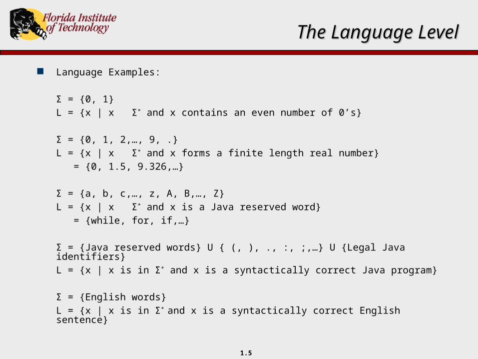
Language Examples:
Σ = 0, 1L = x | x Σ* and x contains an even number of 0’s
Σ = 0, 1, 2,…, 9, .L = x | x Σ* and x forms a finite length real number = 0, 1.5, 9.326,…
Σ = a, b, c,…, z, A, B,…, ZL = x | x Σ* and x is a Java reserved word = while, for, if,…
Σ = Java reserved words U (, ), ., :, ;,… U Legal Java identifiersL = x | x is in Σ* and x is a syntactically correct Java program
Σ = English wordsL = x | x is in Σ* and x is a syntactically correct English sentence
1.6
Problem vs. LanguageProblem vs. Language
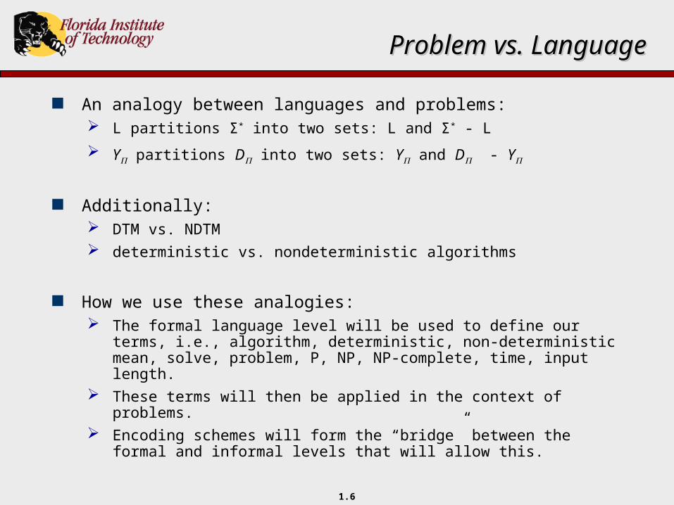
An analogy between languages and problems: L partitions Σ* into two sets: L and Σ* - L
Y partitions D into two sets: Y and D - Y
Additionally: DTM vs. NDTM deterministic vs. nondeterministic algorithms
How we use these analogies: The formal language level will be used to define our
terms, i.e., algorithm, deterministic, non-deterministic mean, solve, problem, P, NP, NP-complete, time, input length.
These terms will then be applied in the context of problems.
Encoding schemes will form the “bridge” between the formal and informal levels that will allow this.
1.7
Encoding SchemesEncoding Schemes
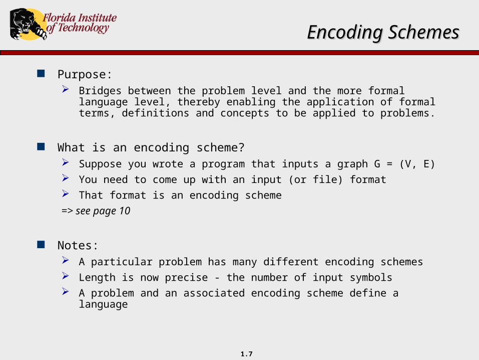
Purpose: Bridges between the problem level and the more formal
language level, thereby enabling the application of formal terms, definitions and concepts to be applied to problems.
What is an encoding scheme? Suppose you wrote a program that inputs a graph G = (V,
E) You need to come up with an input (or file) format That format is an encoding scheme
=> see page 10
Notes: A particular problem has many different encoding schemes Length is now precise - the number of input symbols A problem and an associated encoding scheme define a
language
1.8
Encoding Schemes, cont.Encoding Schemes, cont.
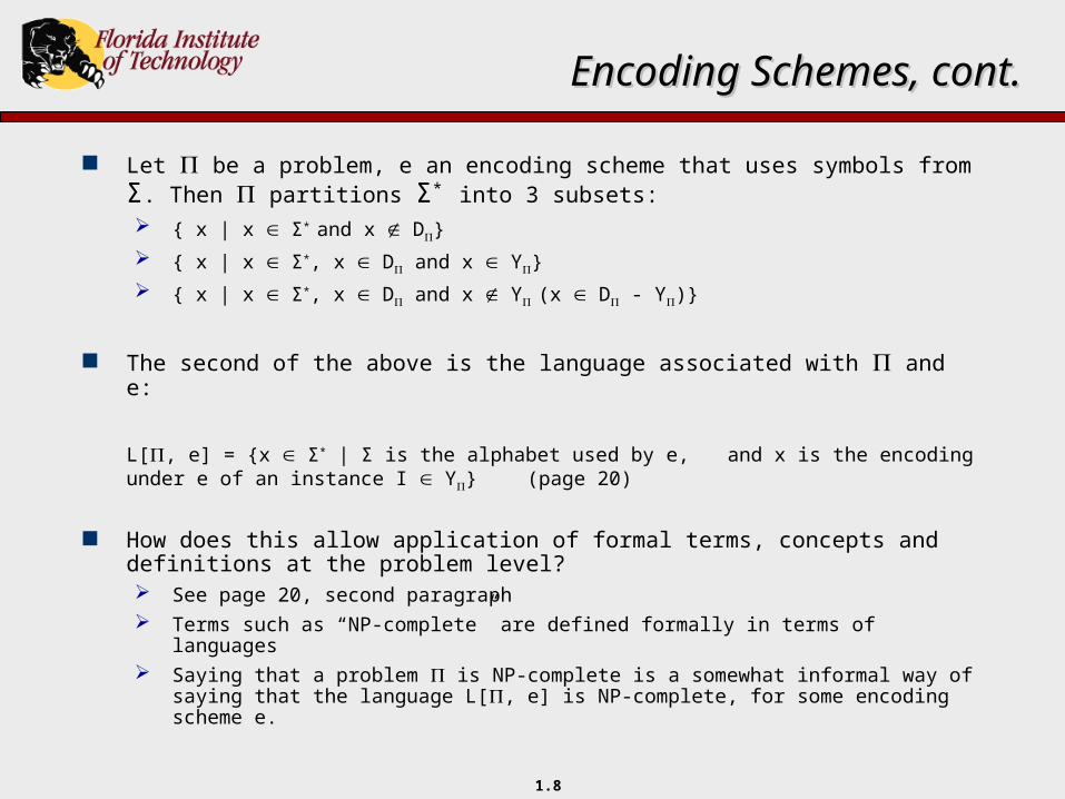
Let be a problem, e an encoding scheme that uses symbols from Σ. Then partitions Σ* into 3 subsets: x | x Σ* and x D
x | x Σ*, x D and x Y
x | x Σ*, x D and x Y (x D - Y)
The second of the above is the language associated with and e:
L[, e] = x Σ* | Σ is the alphabet used by e,and x is the encoding under e of an instance I
Y (page 20)
How does this allow application of formal terms, concepts and definitions at the problem level? See page 20, second paragraph Terms such as “NP-complete” are defined formally in terms of
languages Saying that a problem is NP-complete is a somewhat informal way of
saying that the language L[, e] is NP-complete, for some encoding scheme e.
1.9
Encoding Schemes, cont.Encoding Schemes, cont.
A problem can have many encoding schemes
The previous page suggests our results for a problem are encoding dependent
But is this true? Could a property hold for a problem under one encoding scheme,
but not another? Yes!
Example #1: Input a graph G = (V, E) and for each pair of vertices output an
indication of whether or not the two vertices are adjacent. Adjacency matrix: O(n) (n = input length) Vertex-edge list: O(n2) (no edges)
Note that the encoding scheme does make a difference
1.10
Encoding Schemes, cont.Encoding Schemes, cont.
Example #2: Input a positive integer n and output all binary numbers between 0 and n-1 Input n in binary: O(m2m) (m = input length) Input n in unary: O(log(m)2log(m)) = O(mlogm)
Note that the encoding scheme makes a dramatic difference in running time, i.e., polynomial vs. exponential
The second encoding scheme is unnecessarily padding the input, and is therefore said to be unreasonable
Reasonable encoding schemes are: Concise (relative to how a computer stores things) Decodable (in polynomial time, pages 10, 21)
We do not want the fact that a problem is NP-complete or solvable in polynomial time to depend on a specific encoding scheme Hence, we restrict ourselves to reasonable encoding schemes Comes naturally, unreasonable encoding schemes will look suspicious
1.11
Encoding Schemes and Input Length.Encoding Schemes and Input Length.
The running time of an algorithm, or the computational complexity of a problem is typically expressed as a function of the length of a given instance. O(n2) Ω (n3)
In order to talk about the computational complexity of a problem or the running time of an algorithm, we need to associate a length with each instance.
Every problem will have an associated length function:
LENGTH: D Z+
which must be encoding-scheme independent, i.e., “polynomial related” to the input lengths we would obtain from a reasonable encoding scheme (see page 19 for a definition). This ensures that the length function is also reasonable and that
complexity results for a problem are consistent with those for an associated encoded language.
1.12
Input Length FunctionInput Length Function
Recall the CLIQUE problem:
CLIQUE
INSTANCE: A Graph G = (V, E) and a positive integer J <= |V|.
QUESTION: Does G contain a clique of size J or more?
What would be a reasonable length function? # of vertices
# of edges
# of vertices + # of edges
Which would be polynomial related to a reasonable encoding scheme? Note that the first and last differ quite substantially,
although not exponentially.
1.13
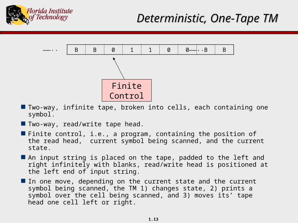
…….. ……..
Two-way, infinite tape, broken into cells, each containing one symbol.
Two-way, read/write tape head. Finite control, i.e., a program, containing the position of the read head, current symbol being scanned, and the current state.
An input string is placed on the tape, padded to the left and right infinitely with blanks, read/write head is positioned at the left end of input string.
In one move, depending on the current state and the current symbol being scanned, the TM 1) changes state, 2) prints a symbol over the cell being scanned, and 3) moves its’ tape head one cell left or right.
FiniteControl
B B 0 1 1 0 0 B B
Deterministic, One-Tape TMDeterministic, One-Tape TM
1.14
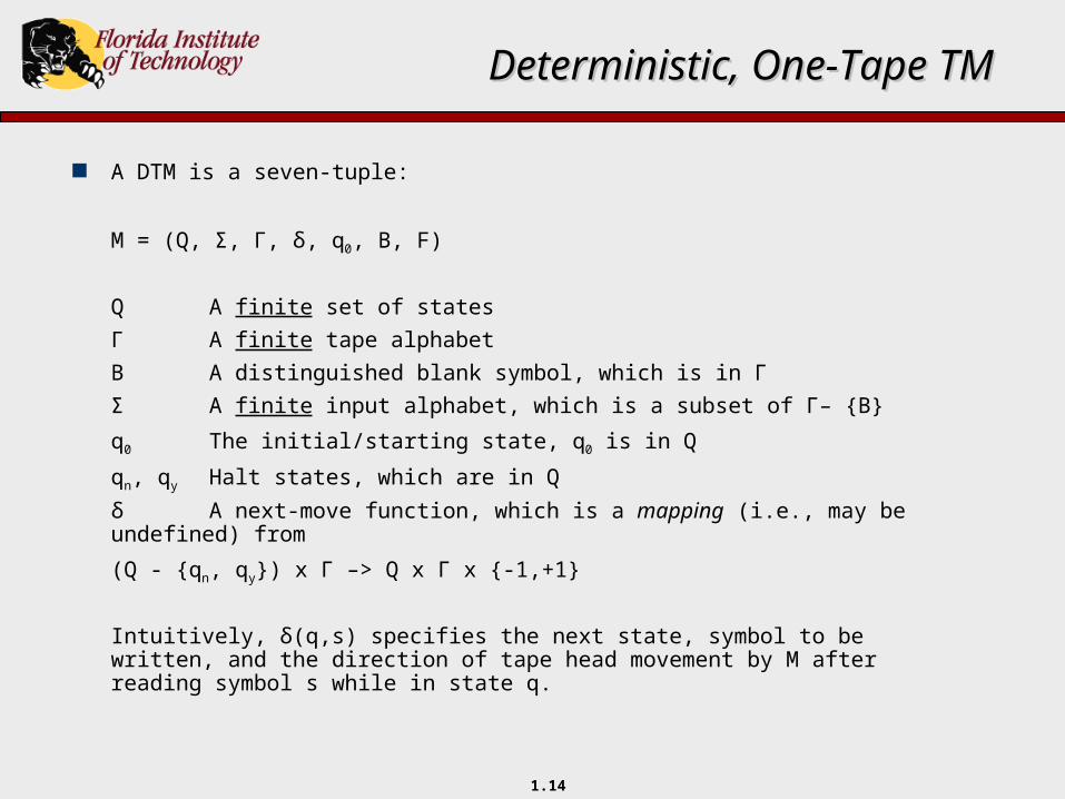
A DTM is a seven-tuple:
M = (Q, Σ, Γ, δ, q0, B, F)
Q A finite set of states
Γ A finite tape alphabet
B A distinguished blank symbol, which is in Γ
Σ A finite input alphabet, which is a subset of Γ– B
q0 The initial/starting state, q0 is in Q
qn, qy Halt states, which are in Q
δ A next-move function, which is a mapping (i.e., may be undefined) from
(Q - qn, qy) x Γ –> Q x Γ x -1,+1
Intuitively, δ(q,s) specifies the next state, symbol to be written, and the direction of tape head movement by M after reading symbol s while in state q.
Deterministic, One-Tape TMDeterministic, One-Tape TM
1.15
DTM DefinitionsDTM Definitions
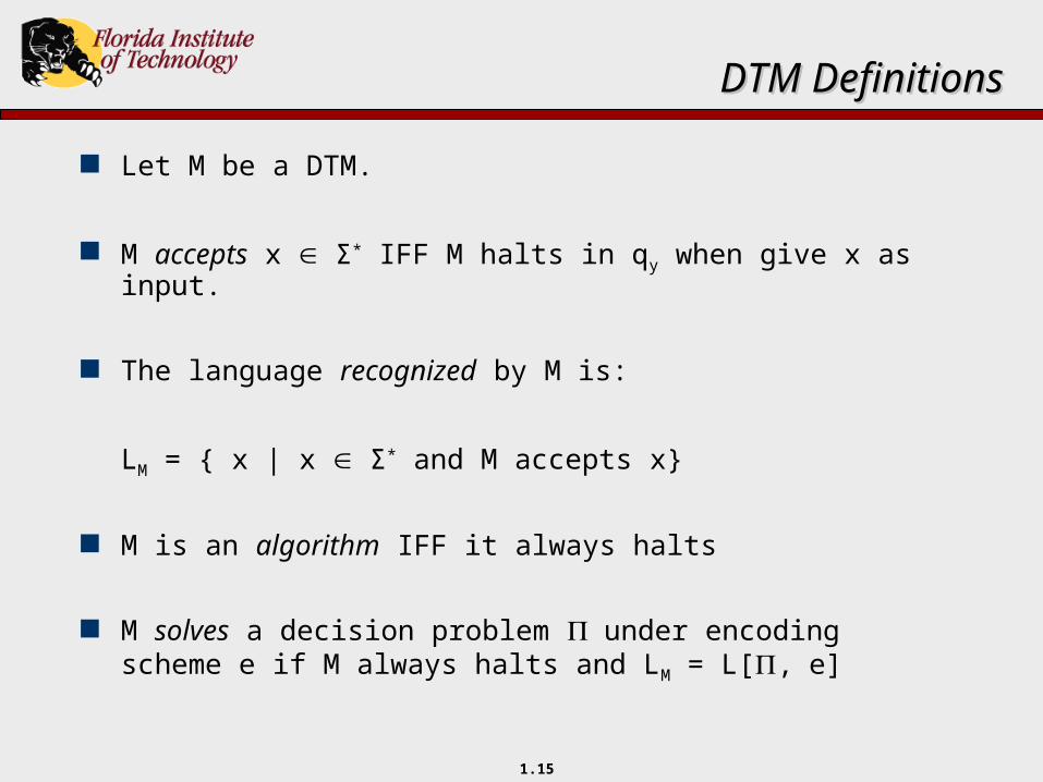
Let M be a DTM.
M accepts x Σ* IFF M halts in qy when give x as input.
The language recognized by M is:
LM = x | x Σ* and M accepts x
M is an algorithm IFF it always halts
M solves a decision problem under encoding scheme e if M always halts and LM = L[, e]
1.16
DTM Definitions, cont.DTM Definitions, cont.
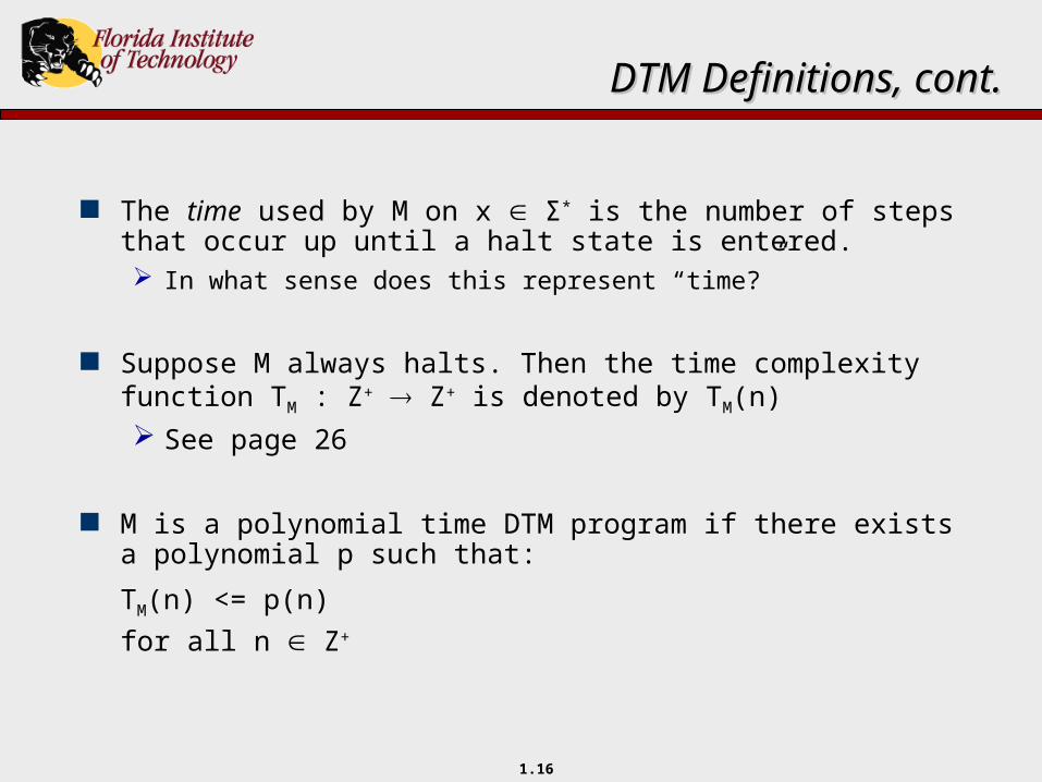
The time used by M on x Σ* is the number of steps that occur up until a halt state is entered. In what sense does this represent “time?”
Suppose M always halts. Then the time complexity function TM : Z+ Z+ is denoted by TM(n) See page 26
M is a polynomial time DTM program if there exists a polynomial p such that:
TM(n) <= p(n)
for all n Z+
1.17
Definition of PDefinition of P
Definition:
P = L : There exists a polynomial-time DTM M such that L = LM
If L[, e] P then we say that belongs to P under e.
What are the implications for if L[, e] P? The problem can be solved in polynomial time
1.18
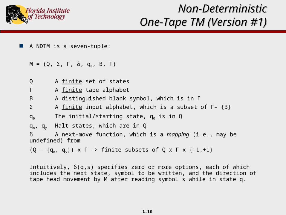
A NDTM is a seven-tuple:
M = (Q, Σ, Γ, δ, q0, B, F)
Q A finite set of states
Γ A finite tape alphabet
B A distinguished blank symbol, which is in Γ
Σ A finite input alphabet, which is a subset of Γ– B
q0 The initial/starting state, q0 is in Q
qn, qy Halt states, which are in Q
δ A next-move function, which is a mapping (i.e., may be undefined) from
(Q - qn, qy) x Γ –> finite subsets of Q x Γ x -1,+1
Intuitively, δ(q,s) specifies zero or more options, each of which includes the next state, symbol to be written, and the direction of tape head movement by M after reading symbol s while in state q.
Non-DeterministicNon-DeterministicOne-Tape TM (Version #1)One-Tape TM (Version #1)
1.19
NDTM DefinitionsNDTM Definitions
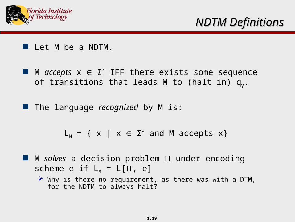
Let M be a NDTM.
M accepts x Σ* IFF there exists some sequence of transitions that leads M to (halt in) qy.
The language recognized by M is:
LM = x | x Σ* and M accepts x
M solves a decision problem under encoding scheme e if LM = L[, e] Why is there no requirement, as there was with a DTM,
for the NDTM to always halt?
1.20
NDTM DefinitionsNDTM Definitions
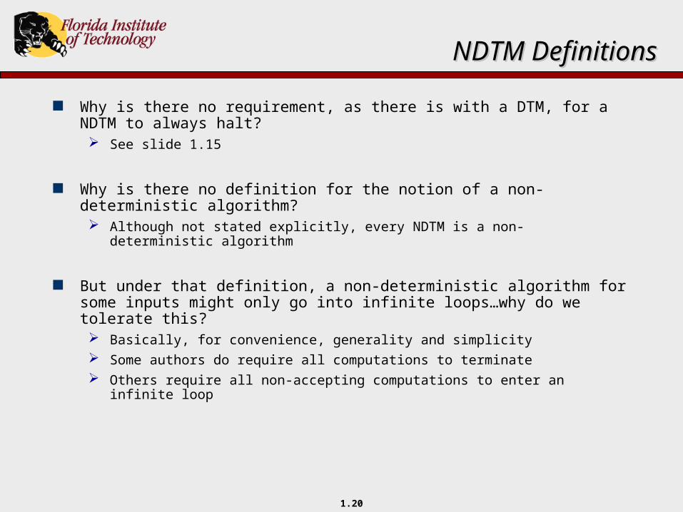
Why is there no requirement, as there is with a DTM, for a NDTM to always halt? See slide 1.15
Why is there no definition for the notion of a non-deterministic algorithm? Although not stated explicitly, every NDTM is a non-
deterministic algorithm
But under that definition, a non-deterministic algorithm for some inputs might only go into infinite loops…why do we tolerate this? Basically, for convenience, generality and simplicity Some authors do require all computations to terminate Others require all non-accepting computations to enter an
infinite loop
1.21
DTMs vs. NDTMsDTMs vs. NDTMs
A DTM is both a language defining device and an intuitive model of computation. A computer program can solve a problem in polynomial time IFF
and DTM can. Anything computable by a DTM is computable by a computer
program.
A NDTM is a language defining device, but not so much a good intuitive model of computation, i.e., it is not clear on the surface that anything “doable” by a NDTM is “doable” by a computer program. In fact, the first is NOT clear at all! How a NDTM “computes” is not even clear, at least in a real-
world sense.
=> For out purposes, it is not as important to think of a NDTM as a “practical” computing device, so much as a language defining device.
1.22
NDTM Definitions, cont.NDTM Definitions, cont.
The time used by M to accept x LM is:
min i | M accepts x in i transitions
Then the time complexity function TM : Z+ Z+ is denoted by TM(n)
See page 31
M is a polynomial time NDTM program if there exists a polynomial p such that:
TM(n) <= p(n)
for all n >= 1.
1.23
NDTM Definitions, cont.NDTM Definitions, cont.
Note that the time complexity function only depends on accepting computations. In fact, if no inputs of a particular size n are accepted, the complexity
function is 1, even if some computations go into an infinite loop.
Why? Aren’t we concerned about the time required for non-accepted strings? The time complexity function could be modified to reflect all inputs We could even require every path in the NDTM to terminate (some authors do
this) Neither of these changes would ultimately matter (I.e., we could convert a
NDTM with the first type of polynomial complexity bound to a NDTM with the second type of polynomial complexity bound and visa versa)
The books model of a NDTM allows infinite computations for convenience - its easy to describe their version of a NDTM, and showing problems are in NP. To accommodate this, the time complexity function only reflects accepting
computations
Note that we could have defined P based only on accepting computations. Altough equivalent, it would be less intuitive (some authors do this)
1.24
Definition of NPDefinition of NP
Definition:
NP = L : There exists a polynomial-time NDTM program M
such that L = LM
If L[, e] NP then we say that belongs to NP under e.
How would one show that a language is in NP? Give a polynomial time NDTM for it (wow!)
What are the implications for if L[, e] NP? How useful or important are problems in NP? Not as clear in this case…
1.25
DTMs vs. NDTMsDTMs vs. NDTMs
Lemma: Every polynomial-time DTM is a polynomial-time NDTM.
Proof: Observe that every DTM is a NDTM If DTM runs in TM(n) deterministic time, then it runs in TM(n)
non-deterministic time, by definition (the reader can verify that the latter is less than the former, i.e., TND
M(n) <= TdM(n).
Therefore, if a DTM runs in deterministic polynomial time, then it runs in non-deterministic polynomial time.
Theorem: P NPProof:
Suppose L P By definition, there exists a polynomial-time DTM M such that L
= LM
By the lemma, M is also a polynomial-time NDTM such that L = LM
Hence, L NP
1.26
DTMs vs. NDTMsDTMs vs. NDTMs
Theorem: If L NP then there exists a polynomial p and a DTM M such that L = LM and TM(n) <= O(2p(n)).
Proof: Let M be a NDTM where L = LM Let q(n) be a polynomial-time bound on M Let r be the maximum number of options provided by δ, i.e:
r = max |S| : q Q, s Γ, and δ(q,s) = S
Proof: If x LM and |x| = n, then There is a “road map” of length <= q(n) for getting to qy
There are rq(n) road maps of length <= q(n) A (3-tape) DTM M’ generates and tries each road map M’ operates in (approximately) O(q(n)rq(n)) time, which is
O(2p(n)) for some p(n).
1.27
DTMs vs. NDTMsDTMs vs. NDTMs
Question: Could this DTM simulation of a NDTM be improved to run in polynomial
time? Only if P = NP
Observations: The preceding proof differs slightly from that given in the book, due to
the different NDTM model Non-deterministic algorithms are starting to look like they might be
useful for realistic problems, i.e., those using deterministic exponential time algorithms.
Note the “exhaustive search” nature of the simulation For many problem in NP, exhaustive search is the only non-deterministic
algorithm
Additional question: Why didn’t we just define P as problems solvable by polynomial
time DTMS, and NP as problems solvable by exponential time DTMS, and then just observe that P is a subset of NP….hmmm….requires more thought…
1.28
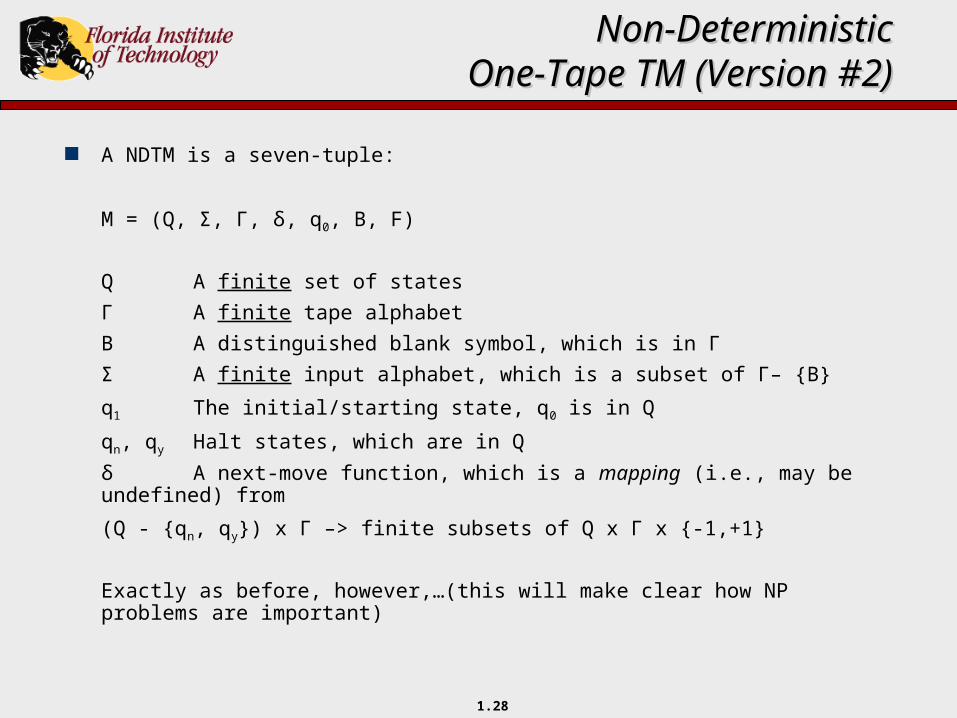
A NDTM is a seven-tuple:
M = (Q, Σ, Γ, δ, q0, B, F)
Q A finite set of states
Γ A finite tape alphabet
B A distinguished blank symbol, which is in Γ
Σ A finite input alphabet, which is a subset of Γ– B
q1 The initial/starting state, q0 is in Q
qn, qy Halt states, which are in Q
δ A next-move function, which is a mapping (i.e., may be undefined) from
(Q - qn, qy) x Γ –> finite subsets of Q x Γ x -1,+1
Exactly as before, however,…(this will make clear how NP problems are important)
Non-DeterministicNon-DeterministicOne-Tape TM (Version #2)One-Tape TM (Version #2)
1.29
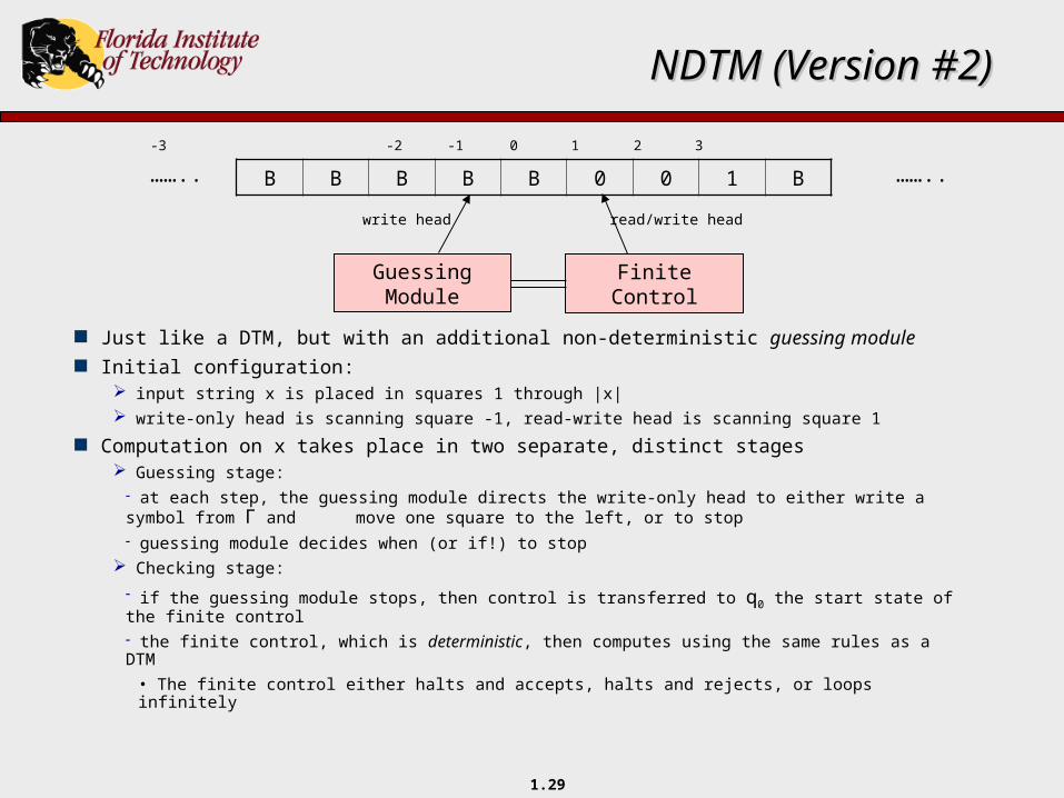
-3 -2 -1 0 1 2 3
…….. ……..
Just like a DTM, but with an additional non-deterministic guessing module Initial configuration:
input string x is placed in squares 1 through |x| write-only head is scanning square -1, read-write head is scanning square 1
Computation on x takes place in two separate, distinct stages Guessing stage: at each step, the guessing module directs the write-only head to either write a symbol from Γ and move one square to the left, or to stop guessing module decides when (or if!) to stop
Checking stage: if the guessing module stops, then control is transferred to q0 the start state of the finite control the finite control, which is deterministic, then computes using the same rules as a DTM
• The finite control either halts and accepts, halts and rejects, or loops infinitely
B B B B B 0 0 1 B
NDTM (Version #2)NDTM (Version #2)
GuessingModule
FiniteControl
write head read/write head
1.30
NDTM (Version #2)NDTM (Version #2)
Notes:
The guessing module can guess any string from Γ* Hmmm…so what exactly does a guessing module look like?
The guessing module allows for an infinite # of computations This explains the need for the time complexity function to only
consider accepting computations.
We could put a bound on the guess to eliminate this, but its easier to describe the NDTM without it, and it doesn’t matter anyway (class NP stays the same).
The guessed string is usually used in the second stage
For a given input string x, there are an infinite number of computations of a NDTM
1.31
NDTM (Version #2)NDTM (Version #2)
M accepts x Σ* if there exists a guess x Γ* that brings M to qy
Note that this is basically the same as our our definition of string acceptance with Version #1
The time to accept x Σ* … same as before (see slide 1.21)
All definitions and theorems proved about the first verson of NDTMs still hold: LM, TM(n), NP P NP (verify this one) If L NP then there exists a polynomial p and a DTM
such that L = LM and TM(n) <= O(2p(n))
1.32
NDTM (Version #2)NDTM (Version #2)
Are the two different versions of NDTMs equivalent? There exists a NDTM version #1 that accepts L IFF there exist a
NDTM version #2 that accepts L Prove this as an exercise
But are the models equivalent with respect to time complexity? Do the two models define the same class NP? Yes!
Why do Garey and Johnson use Version #2? Convenience At the problem level, it is easer to show a problem (or
language) is in NP
How does one show a problem (or language) is in P?
How does one show a problem (or language) is in NP?
1.33
Proving a Problem NP-CompleteProving a Problem NP-Complete(overview)(overview)
To show a problem is NP-complete we must show: NP ’ , for all ’ NP
To show NP we need to give a NDTM, or rather, a non-deterministic algorithm for , that operates in polynomial time.
For most decision problems, Garey and Johnson’s NDTM model makes this easy.
1.34
Proving a Problem is in NPProving a Problem is in NP
Another way to look at model #2:
NP IFF there exits a deterministic polynomial time algorithm A such that: If I Y then there exists a “structure” S such that
(I,S) is accepted by A If I Y then for any “structure” S, it will always be
the case that (I,S) is rejected by A
1.35
Example #1: TSP Example #1: TSP
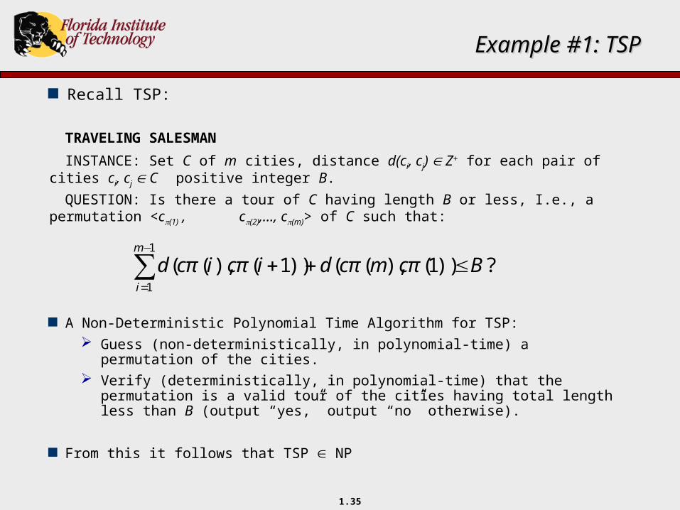
Recall TSP:
TRAVELING SALESMAN
INSTANCE: Set C of m cities, distance d(ci, cj) Z+ for each pair of cities ci, cj C positive integer B.
QUESTION: Is there a tour of C having length B or less, I.e., a permutation <c(1) , c(2),…, c(m)> of C such that:
A Non-Deterministic Polynomial Time Algorithm for TSP: Guess (non-deterministically, in polynomial-time) a
permutation of the cities. Verify (deterministically, in polynomial-time) that the
permutation is a valid tour of the cities having total length less than B (output “yes,” output “no” otherwise).
From this it follows that TSP NP
∑−
=
≤++1
1
?))1(),(())1(),((m
i
Bcmcdicicd ππππ
1.36
Example #2: Clique Example #2: Clique
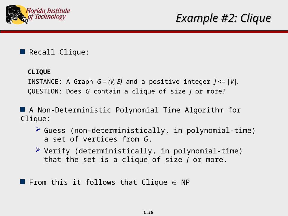
Recall Clique:
CLIQUE
INSTANCE: A Graph G = (V, E) and a positive integer J <= |V|.
QUESTION: Does G contain a clique of size J or more?
A Non-Deterministic Polynomial Time Algorithm for Clique:
Guess (non-deterministically, in polynomial-time) a set of vertices from G.
Verify (deterministically, in polynomial-time) that the set is a clique of size J or more.
From this it follows that Clique NP
1.37
Example #3: Graph K-ColorabilityExample #3: Graph K-Colorability
Recall Graph K-Colorability:
GRAPH K-COLORABILITY
INSTANCE: A Graph G = (V, E) and a positive integer K <= |V|.
QUESTION: Is the graph G K-colorable?
A Non-Deterministic Algorithm Polynomial Time for Graph K-colorability:
Guess (non-deterministically, in polynomial-time) a coloring of G.
Verify (deterministically, in polynomial-time) that the coloring is a valid K-coloring of G.
From this it follows that Graph K-colorability NP
1.38
Example #4: SAT Example #4: SAT
Recall Satisfiability:
SATISFIABILITY
INSTANCE: Set U of variables and a collection C of clauses over U.
QUESTION: Is there a satisfying truth assignment for C?
A Non-Deterministic Polynomial Time Algorithm for Satisfiability:
Guess (non-deterministically, in polynomial-time) a truth assignment for the variables in U.
Verify (deterministically, in polynomial-time) that the truth assignment satisfies C.
From this it follows that Satisfiability NP
1.39
Example #5: Non-Tautology Example #5: Non-Tautology
NON-TAUTOLOGY
INSTANCE: Boolean expression E (, , , ).
QUESTION: Is E not a tautology?
A Non-Deterministic Polynomial Time Algorithm for Non-Tautology:
Guess (non-deterministically, in polynomial-time) a truth assignment for E.
Verify (deterministically, in polynomial-time) that the truth assignment does not satisfy E.
From this it follows that Non-Tautology NP
1.40
Example #6: Tautology Example #6: Tautology
TAUTOLOGY
INSTANCE: Boolean expression E (, , , ).
QUESTION: Is E a tautology?
A Non-Deterministic Polynomial Time Algorithm for Tautology:
Guess ?
Verify ?
Is Tautology NP? We do not know!
1.41
Tentative View of the World of NP Tentative View of the World of NP
If P = NP then everything in NP can be solved in deterministic polynomial time.
If P≠ NP then: P NP Everything in P can be solved in deterministic polynomial time
Everything in NP - P is intractable
Hence, given a problem we would like to know if P or NP - P
Unfortunately, we do not know if P = NP or P≠ NP
It does appear that P≠ NP since there are many problem in NP for which nobody has been able to find deterministic polynomial time algorithms
1.42
Tentative View of the World of NP Tentative View of the World of NP
For some problems we can show that P
Unfortunately, we cannot not show that NP - P, at least not without resolving the P =? NP question, which appears to be very difficult
Hence, we will restrict ourselves to showing that for some problems, if P≠ NP then NP - P
Although the theory of NP-completeness assumes that P≠ NP, if it turned out that P = NP, then parts of the theory (i.e., transformations and reductions) can still be used to prove results concerning the relative complexity of problems.
1.43
Polynomial Transformation Polynomial Transformation
A polynomial transformation from a language L1 Σ1*
and to a language L2 Σ2* is a function f: Σ1
* Σ2*
that statisfies the following conditions: There is a polynomial time DTM program that computes f
For all x Σ1*, x L1
* iff and only if f(x) L2*
If there is a polynomial transformation from L1 to L2 then we write L1 L2, read “L1 transforms to L2“
1.44
Polynomial Transformation Polynomial Transformation
The significance of polynomial transformations follows from Lemma 2.1
Lemma 2.1: If L1 L2 and L2 P then L1 P
Proof: Let M be a polynomial time DTM that decides L2 , and let M’ be a polynomial time DTM that computes f. Then M’ and M can be composed to give a polynomial time DTM that decides .
Equivalently, if L1 L2 and L1 P then L2 P
1.45
Polynomial Transformation Polynomial Transformation
Informally, if L1 L2 then it is frequently said that: L1 Is no harder than L2
L2 Is no easier than L1
L2 Is at least as hard as L1
L1 Is as easy as L2
Note that “hard” and “easy” here are only with respect to polynomial v.s. exponential time We could have L1 decidable in 2n time, L2 decidable in
time, but where L1 is not.
€
2 n
1.46
Polynomial Transformation Polynomial Transformation
At the problem level we can regard a polynomial transformation from the decision problem 1 Σ1
* and to a decision problem 2 Σ2
* is a function f : D1
D2 that statisfies the following conditions:
f is computable by a polynomial time algorithm
For all I D1, I Y1 if and only if f ( I) Y2
We will deal with transformations only at the problem level
1.47
Polynomial Transformation Polynomial Transformation
Another helpful factoid concerning transformations:
Lemma 2.2: If L1 L2 and L2 L3 then L1 L3
In other words, polynomial transformations are transitive.
1.48
Definition of NP-Complete Definition of NP-Complete
A decision problem is NP-complete if: NP, and For all other decision problems ’ NP, ’
For many problems, proving the first requirement is easy.
On the surface, the second requirement would appear very difficult to prove, especially given that there are an infinite number of problems in NP.
As will be shown, the second requirement will be established using the following lemma:
Lemma 2.3: If L1 and L2 belong to NP, L1 is NP-complete, and L1 L2 then L2 is NP-complete.
1.49
Definition of NP-Complete, cont. Definition of NP-Complete, cont.
Let be an NP-complete problem
Observation: P If and only if P = NP
(only if) If an NP-complete problem can be solved in
polynomial time, then every problem in NP can be solved in polynomial time (should be clear, by definition). If P then P = NP
If any problem in NP is intractable, then so are all NP-complete problems. If P≠ NP then P (i.e., NP-P), for all NP-complete
problems
1.50
Definition of NP-Complete, cont. Definition of NP-Complete, cont.
Let be an NP-complete problem
Observation: P If and only if P = NP
(if) If every problem in NP can be solved in polynomial
time, then clearly every NP-complete problem can be also, since every NP-complete problem, by definition, is in NP. If P = NP then P, for all NP-complete problems
If any NP-complete problem in NP is intractable, then clearly P ≠ NP. If P (i.e., NP-P) then P ≠ NP, for any NP-complete
problem
1.51
Definition of NP-Complete, cont. Definition of NP-Complete, cont.
Could there be an NP-complete problem that is solvable in polynomial time, but where there is another problem in NP that requires exponential time? No!
For this reason, NP-complete problems are referred to as the “hardest” problems in NP.
1.52
Cooks Theorem - Background Cooks Theorem - Background
Our first NP-completeness proof will not use Lemma 2.3, but all others will.
Recall the Satisfiability problem (SAT)
SATISFIABILITY (SAT)INSTANCE: Set U of variables and a collection C of clauses over U.QUESTION: Is there a satisfying truth assignment for C?
Example #1:
U = u1, u2
C = u1, u2 , u1, u2 Answer is “yes” - satisfiable by make both variables T
Example #2:
U = u1, u2
C = u1, u2 , u1, u2 , u1 Answer is “no”
1.53
Statement of Cook’s Theorem Statement of Cook’s Theorem
Theorem: SAT is NP-complete (Cook).1. SAT NP2. We must show that for all NP, SAT
More formally, for all languages L NP, L L[SAT,e], for some reasonable encoding scheme e
Question: Is Cook’s theorem a polynomial-time transformation?
Answer: Sort of – it is a generic polynomial-time transformation.
Question: But in what sense is it generic?
Answer: It is generic in that, given any specific problem in NP, that problem combined with Cook’s theorem will give a specific polynomial-time transformation.
1.54
Cook’s Theorem Cook’s Theorem
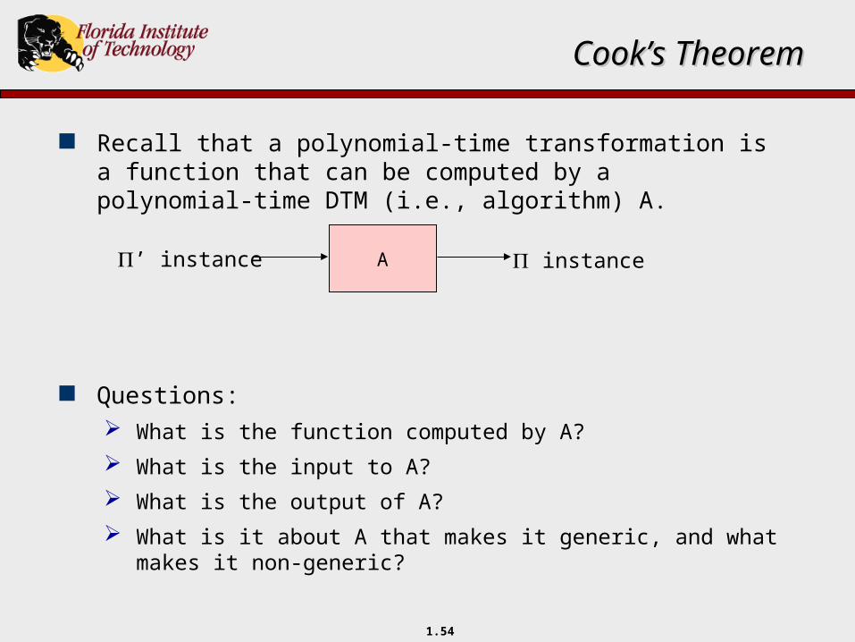
Recall that a polynomial-time transformation is a function that can be computed by a polynomial-time DTM (i.e., algorithm) A.
Questions: What is the function computed by A?
What is the input to A?
What is the output of A?
What is it about A that makes it generic, and what makes it non-generic?
A’ instance instance
1.55
Cook’s Theorem Cook’s Theorem
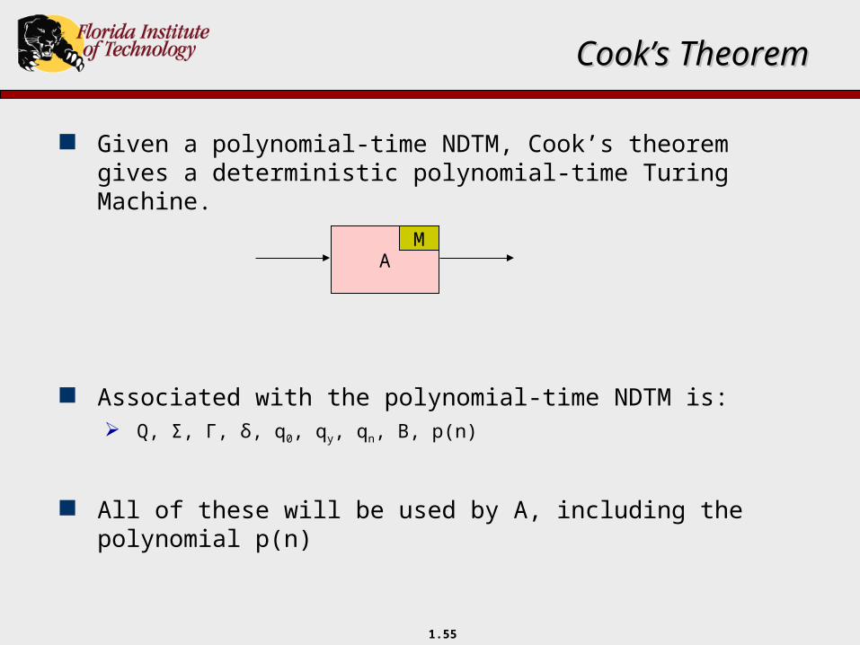
Given a polynomial-time NDTM, Cook’s theorem gives a deterministic polynomial-time Turing Machine.
Associated with the polynomial-time NDTM is: Q, Σ, Γ, δ, q0, qy, qn, B, p(n)
All of these will be used by A, including the polynomial p(n)
AM
1.56
Cook’s Theorem Cook’s Theorem
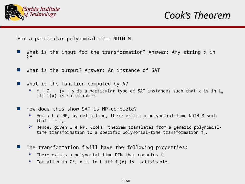
For a particular polynomial-time NDTM M:
What is the input for the transformation? Answer: Any string x in Σ*
What is the output? Answer: An instance of SAT
What is the function computed by A? f : Σ* y | y is a particular type of SAT instance such that x is in
LM iff f(x) is satisfiable.
How does this show SAT is NP-complete? For a L NP, by definition, there exists a polynomial-time NDTM M such
that L = LM. Hence, given L NP, Cooks’ theorem translates from a generic
polynomial-time transformation to a specific polynomial-time transformation fL.
The transformation fLwill have the following properties: There exists a polynomial-time DTM that computes fL
For all x in Σ*, x is in L iff fL(x) is satisfiable.
1.57
Cook’s Theorem Cook’s Theorem
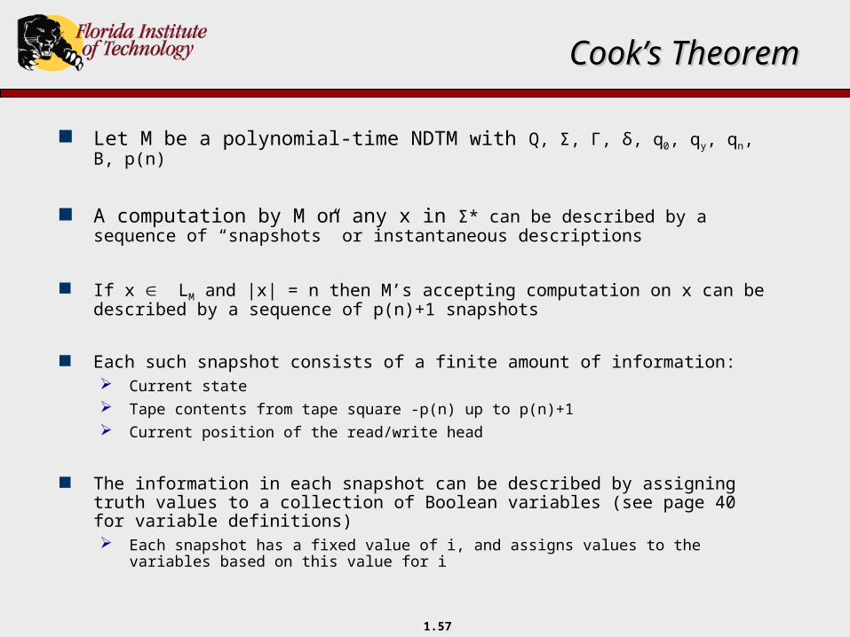
Let M be a polynomial-time NDTM with Q, Σ, Γ, δ, q0, qy, qn, B, p(n)
A computation by M on any x in Σ* can be described by a sequence of “snapshots” or instantaneous descriptions
If x LM and |x| = n then M’s accepting computation on x can be described by a sequence of p(n)+1 snapshots
Each such snapshot consists of a finite amount of information: Current state Tape contents from tape square -p(n) up to p(n)+1 Current position of the read/write head
The information in each snapshot can be described by assigning truth values to a collection of Boolean variables (see page 40 for variable definitions) Each snapshot has a fixed value of i, and assigns values to the
variables based on this value for i
1.58
Cook’s Theorem Cook’s Theorem
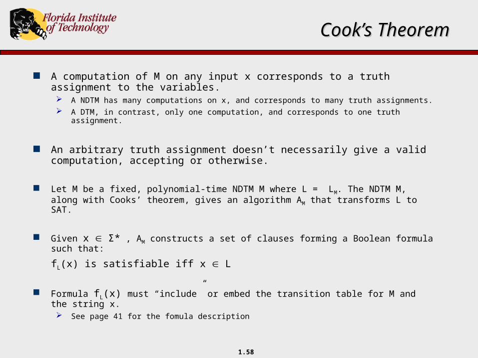
A computation of M on any input x corresponds to a truth assignment to the variables. A NDTM has many computations on x, and corresponds to many truth assignments. A DTM, in contrast, only one computation, and corresponds to one truth
assignment.
An arbitrary truth assignment doesn’t necessarily give a valid computation, accepting or otherwise.
Let M be a fixed, polynomial-time NDTM M where L = LM. The NDTM M, along with Cooks’ theorem, gives an algorithm AM that transforms L to SAT.
Given x Σ* , AM constructs a set of clauses forming a Boolean formula such that:
fL(x) is satisfiable iff x L
Formula fL(x) must “include” or embed the transition table for M and the string x. See page 41 for the fomula description
1.59
Cook’s Theorem Cook’s Theorem
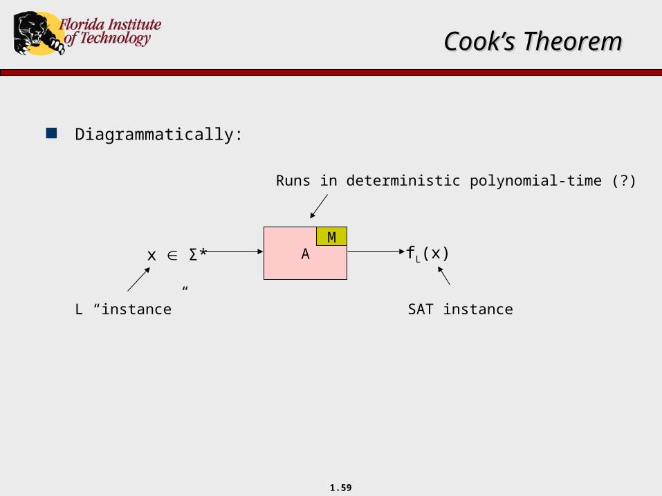
Diagrammatically:
AM
x Σ* fL(x)
L “instance” SAT instance
Runs in deterministic polynomial-time (?)
1.60
Cook’s Theorem Cook’s Theorem
If there is an accepting computation of M on x, then are the clauses satisfiable?
If the clauses are satisfiable, then is there an accepting computation of M on x?
How does each group of clauses work?
Where is the guess in all of the clauses, or how is it represented? See the last sentence on page 40. Wow! The assignments to the variables in the third group of clauses at time 0
on tape squares -p(n) to -1 tells us what the guess is.
Suppose is satisfiable. Can the non-deterministic guess be determined from the satisfying truth assignment? Yes, each satisfying truth assignment defines a guess and a
computation Note that the NDTM used in the construction could be based on
either model #1 or model #2
1.61
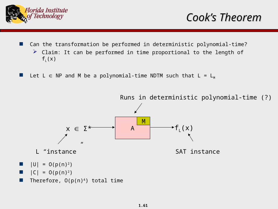
Cook’s Theorem Cook’s Theorem
Can the transformation be performed in deterministic polynomial-time? Claim: It can be performed in time proportional to the length of
fL(x)
Let L NP and M be a polynomial-time NDTM such that L = LM
|U| = O(p(n)2) |C| = O(p(n)2) Therefore, O(p(n)4) total time
AM
x Σ* fL(x)
L “instance” SAT instance
Runs in deterministic polynomial-time (?)


