11_Critical State Model

324

CHAPTER 11A CRITICAL STATE MODEL TO INTERPRET SOIL BEHAVIOR

11.0 INTRODUCTION

In this chapter, a simple soil model that combines consolidation and shear strength to interpret and pre-dict soil responses to static loading is presented. When you complete this chapter, you should be able to:

• Estimate failure stresses for soil.

• Estimate strains at failure.

• Understand the relationship among soil parameters.

• Estimate whether drained or undrained condition would be critical for practical problems.

• Estimate whether a soil will show a peak shear stress or not.

• Predict stress–strain characteristics of soils from a few parameters obtained from simple soil tests.

• Evaluate possible soil stress states and failure if the loading on a geotechnical system were to change.

You will make use of all the materials you studied in Chapters 2 to 10, but particularly:

• Index properties

• Effective stresses, stress invariants, and stress paths

• Primary consolidation

• Shear strength

Importance

So far, we have painted individual pictures of soil behavior. We have looked at the physical character-istics of soils, one-dimensional fl ow of water through soils, stresses in soils from surface loads, effective stresses, stress paths, one-dimensional consolidation, and shear strength. You know that if you consoli-date a soil to a higher stress state than its current one, the shear strength of the soil will increase. But the amount of increase depends on the soil type, the loading conditions (drained or undrained condition), and the stress paths. Therefore, the individual pictures should all be linked together. But how?

In this chapter, we are going to take the individual pictures and build a mosaic that will provide a basis for us to interpret and anticipate soil behavior. Our mosaic is mainly intended to unite con-solidation and shear strength. Real soils, of course, require a complex mosaic, not only because soils are natural, complex materials, but also because the loads and loading paths cannot be anticipated accurately.

Our mosaic will provide a simple framework to describe, interpret, and anticipate soil responses to various loadings. The framework is essentially a theoretical model based on critical state soil mechanics—critical state model (Schofi eld and Wroth, 1968). Laboratory and fi eld data, especially results from soft, normally consolidated clays, lend support to the underlying concepts embodied in the development of the critical state model. The emphasis in this chapter will be on using the critical state model to provide a gen-eralized understanding of soil behavior rather than on the mathematical formulation.

The critical state model (CSM) we are going to study is a simplifi cation and an idealization of soil behavior. However, the CSM captures the behavior of soils that are of greatest importance to geotechni-cal engineers. The central idea in the CSM is that all soils will fail on a unique failure surface in (p9, q, e) space (see book cover). Thus, the CSM incorporates volume changes in its failure criterion, unlike the Mohr–Coulomb failure criterion, which defi nes failure only as the attainment of the maximum stress obliquity. According to the CSM, the failure stress state is insuffi cient to guarantee failure; the soil struc-ture must also be loose enough.

The CSM is a tool to make estimates of soil responses when you cannot conduct suffi cient soil tests to completely characterize a soil at a site or when you have to predict the soil’s response from changes in loading during and after construction. Although there is a debate about the application of the CSM to real soils, the ideas behind the CSM are simple. It is a very powerful tool to get insights into soil behavior, especially in the case of the “what-if” situation. There is also a plethora of soil models in the literature that have critical state as their core. By studying the CSM, albeit a simplifi ed version in this chapter, you will be able to better understand these other soil models.

A practical scenario is as follows. An oil tank is to be constructed on a soft alluvial clay. It was decided that the clay would be preloaded with a circular embankment imposing a stress at least equal to the total applied stress of the tank when fi lled. Wick drains (Chapter 9) are to be used to accelerate the consolidation process. The foundation for the tank is a circular slab of concrete, and the purpose of the preloading is to reduce the total settlement of the foundation. You are required to advise the owners on how the tank should be fi lled during preloading to prevent premature failure and to achieve the desired settlement. After preloading, the owners decided to increase the height of the tank. You are requested to determine whether the soil has enough shear strength to support an additional increase in tank height, and if so, the amount of settlement that can be expected. The owners are reluctant to fi nance any further preloading and soil testing.

11.1 DEFINITIONS OF KEY TERMS

Preconsolidation ratio (Ro) is the ratio by which the current mean effective stress in the soil was exceeded in the past (Ro 5 p rc /p ro, where p rc is the preconsolidation mean effective stress, or, simply, pre-consolidation stress, and p ro is the current mean effective stress).

Compression index (l) is the slope of the normal consolidation line in a plot of void ratio versus the natural logarithm of mean effective stress.

Unloading/reloading index, or recompression index (k), is the average slope of the unloading/reloading curves in a plot of void ratio versus the natural logarithm of mean effective stress.

Critical state line (CSL) is a line that represents the failure state of soils. In (p9, q) space, the critical state line has a slope M, which is related to the friction angle of the soil at the critical state. In (e, ln p9) space, the critical state line has a slope l, which is parallel to the normal consolidation line. In three-dimensional (p9, q, e) space (see book cover), the critical state line becomes a critical state surface.

11.2 QUESTIONS TO GUIDE YOUR READING

1. What is soil yielding?

2. What is the difference between yielding and failure in soils?

3. What parameters affect the yielding and failure of soils?

4. Does the failure stress depend on the consolidation pressure?

5. What are the critical state parameters, and how can you determine them from soil tests?

6. Are strains important in soil failure?

11.2 QUESTIONS TO GUIDE YOUR READING 325

326 CHAPTER 11 A CRITICAL STATE MODEL TO INTERPRET SOIL BEHAVIOR

7. What are the differences in the stress–strain responses of soils due to different stress paths?

8. What are the differences in behavior of soils under drained and undrained conditions?

9. Are the results from triaxial compression tests and direct simple shear the same? If not, how do I estimate the shear strength of a soil under direct simple shear from the results of triaxial compression, or vice versa?

10. How do I estimate the shear strength of a soil in the fi eld from the results of lab tests?

11. How do loading (stress) paths affect the response of soils?

11.3 BASIC CONCEPTS

Interactive Concept Learning

Access www.wiley.com/college/budhu, click on Chapter 11, and download an interactive lesson (criticalstate.zip) (1) to learn the basic concepts of the critical state model, (2) to calculate yield and failure stresses and strains, (3) to calculate yield stresses and strains, and (4) to predict stress–strain responses for both drained and undrained conditions.

11.3.1 Parameter Mapping

In our development of the basic concepts on critical state, we are going to map certain plots we have studied in Chapters 8, 9, and 10 using stress and strain invariants and concentrate on a saturated soil under axisymmetric loading. However, the concepts and method hold for any loading condition. Rather than plotting s rn versus t, we will plot the data as p9 versus q (Figure 11.1a). This means that you must know the principal stresses acting on the element. For axisymmetric (triaxial) condition, you only need to know two principal stresses.

The Coulomb failure line in (s9n, t) space of slope f9cs 5 tan21[tcs/(s9n)f] is now mapped in (p9, q) space as a line of slope M 5 qf /p rf , where the subscript f denotes failure. Instead of a plot of s9z versus e, we will plot the data as p9 versus e (Figure 11.1b), and instead of s9n (log scale) versus e, we will plot p9 (ln scale) versus e (Figure 11.1c). The p9 (ln scale) versus e plot will be referred to as the (ln p9, e) plot.

We will denote the slope of the normal consolidation line (NCL) in the plot of p9 (ln scale) versus e as l and the unloading/reloading (URL) line as k. The NCL is a generic normal consolidation line. In the initial development of the CSM in this textbook, the NCL is the same as the isotropic consolidation line (ICL). Later, we will differentiate ICL from the one-dimensional consolidation line (KoCL). All these consolidation lines have the same slope. There are now relationships between f rcs and M, Cc and l, and Cr and k. The relationships for the slopes of the normal consolidation line, l, and the unloading/reloading line, k, are

l 5

Cc

ln 110 2 5Cc

2.35 0.434 Cc

(11.1)

k 5

Cr

ln 110 2 5Cr

2.35 0.434 Cr

(11.2)

Both l and k are positive for compression. For many soils, k/l has values within the range 110 to 15. We will

formulate the relationship between f rcs and M later. The overconsolidation ratio using stress invariants, called preconsolidation ratio, is

Ro 5p rcp ro

(11.3)

11.3 BASIC CONCEPTS 327

where p9o is the initial mean effective stress or overburden mean pressure and p9c is the preconsolidation mean effective stress or, simply, preconsolidation stress. The preconsolidation ratio, Ro, defi ned by Equa-tion (11.3) is not equal to OCR [Equation (9.13)] except for soils that have been isotropically consolidated.

EXAMPLE 11.1 Calculation of l and k from One-Dimensional Consolidation Test Results

The results of one-dimensional consolidation tests on a clay are Cc 5 0.69 and Cr 5 0.16. Calculate l and k.

Strategy This solution is a straightforward application of Equations (11.1) and (11.2).

Solution 11.1

Step 1: Calculate l and k.

l 5Cc

2.35

0.692.3

5 0.3

k 5Cr

2.35

0.162.3

5 0.07

FIGURE 11.1 Mapping of strength and consolidation parameters.

Failure line or critical state line: M =

Failure line: = tan–1–––––

qf–––p'f

q

e

p'

e

(a)

(b)

(c)

e

σ'n (log scale) p' (In scale)

e�

�Cr

Cr

Cc

φ'cs

φ'cs

τcs

τ

σ'n

λ

(σ'z)f

Normal effective stress, σ'n Mean effective stress, p'

She

ar s

tres

s

Dev

iato

ric

stre

ss


11.3.2 Failure Surface

The fundamental concept in CSM is that a unique failure surface exists in (p9, q, e) space (see book cover), which defi nes failure of a soil irrespective of the history of loading or the stress paths followed. Failure and critical state are synonymous. We will refer to the failure line as the critical state line (CSL) in this chapter. You should recall that critical state is a constant stress state characterized by continuous shear deformation at constant volume. In stress space (p9, q) the CSL is a straight line of slope M 5 Mc, for compression, and M 5 Me, for extension (Figure 11.2a). Extension does not mean tension but refers to the case where the lateral stress is greater than the vertical stress. There is a corresponding CSL in (p9, e) space (Figure 11.2b) or (ln p9, e) space (Figure 11.2c) that is parallel to the normal consolidation line.

We can represent the CSL in a single three-dimensional plot with axes p9, q, e (see book cover), but we will use the projections of the failure surface in the (q, p9) space and the (p9, e) space for sim-plicity. The failure surface shown on the book cover does not defi ne limiting stresses as Coulomb or Mohr–Coulomb failure surfaces. It is a failure surface based on a particular set of stress and strain invariants [p, q, εp, εq; see Equations (8.1) to (8.5)] that leads to energy balance (input energy 5 output or dissipated energy) for soil as a continuum. Coulomb and Mohr–Coulomb failure surfaces are failure surfaces or planes in which the soil masses above and below them are rigid bodies. These failure planes are planes of discontinuity.

11.3.3 Soil Yielding

You should recall from Chapter 7 (Figure 7.8) that there is a yield surface in stress space that separates stress states that produce elastic responses from stress states that produce plastic responses. We are going to use the yield surface in (p9, q) space (Figure 11.3) rather than (s91, s93) space so that our interpretation of soil responses is independent of the axis system.

FIGURE 11.2 Critical statelines, normal compression,and unloading/reloading lines.

URL

Mc

Me

CSL

CSL

p'

q

e

(a)

(b)

NCL

CSL

URL

p' (In scale)

e

(c)

NCL

CSL

p'

λ

λ

κ


The yield surface is assumed to be an ellipse, and its initial size or major axis is determined by the preconsolidation stress, p9c. Experimental evidence (Wong and Mitchell, 1975) indicates that an elliptical yield surface is a reasonable approximation for soils. The higher the preconsolidation stress, the larger the initial ellipse. We will consider the yield surface for compression, but the ideas are the same for extension except that the minor axis of the elliptical yield surface in extension is smaller than in compression.

All combinations of q and p9 that are within the yield surface, for example, point A in Figure 11.3, will cause the soil to respond elastically. If a combination of q and p9 lies on the initial yield surface (point B, Figure 11.3), the soil yields in a similar fashion to the yielding of a steel bar. Any tendency of a stress combination to move outside the current yield surface is accompanied by an expansion of the current yield surface, such that during plastic loading the stress point (p9, q) lies on the expanded yield surface and not outside, as depicted by C. Effective stress paths such as BC (Figure 11.3) cause the soil to behave elastoplastically.

If the soil is unloaded from any stress state below failure, the soil will respond like an elastic materi-al. As the initial yield surface expands, the elastic region gets larger. Expansion of the initial yield surface simulates strain-hardening materials such as loose sands and normally and lightly overconsolidated clays. The initial yield surface can also contract, simulating strain-softening materials such as dense sands and heavily overconsolidated clays. You can think of the yield surface as a balloon. Blowing up the balloon (applying pressure; loading) is analogous to the expansion of the yield surface. Releasing the air (gas) from the balloon (reducing pressure; unloading) is analogous to the contraction of the yield surface.

The critical state line intersects every yield surface at its crest. Thus, the intersection of the initial

yield surface and the critical state line is at a mean effective stress prc2

, and for the expanded yield surface

it is at prG2

.

11.3.4 Prediction of the Behavior of Normally Consolidated and Lightly Overconsolidated Soils Under Drained Condition

Let us consider a hypothetical situation to illustrate the ideas presented so far. We are going to try to predict how a sample of soil of initial void ratio eo will respond when tested under drained condition in a triaxial apparatus, that is, a standard CD test. You should recall that the soil sample in a CD test is isotropically consolidated and then axial loads or displacements are applied, keeping the cell pressure constant. We are going to consolidate our soil sample up to a maximum mean effective stress p9c, and then unload it to a mean effective stress p9o such that Ro 5 prc /p ro , 2. The limits imposed on Ro are only for presenting the basic ideas on CSM. More details on delineating lightly overconsolidated from heavily overconsolidated soils will be presented in Section 11.7.

On a plot of p9 versus e (Figure 11.4b), the isotropic consolidation path is represented by AC. You should recall from Figure 11.1 that the line AC maps as the normal consolidation line (NCL) of slope l. Because we are applying isotropic loading, the line AC is called the isotropic consolidation line (ICL).

FIGURE 11.3 Expansion of the yield surface.

Expanded yield surface

Initial yield surface in compression

2

CB

AG

p'p'cp'c p'G

Mc

q

A—elastic stress stateB—initial yieldingC—elastoplastic

2

p'G


FIGURE 11.4 Illustrative predicted results from a triaxial CD test on a lightly overconsolidated soil (1 , Ro # 2) using CSM.

ESP

Elastic

q q

qf

S

E

D

F

C GA

O

A

SF

O'

CSL

C

p'f p'

p'o p'G p'p'Cp'E

O' E'

O'E' = elastic axial strain

Elastoplasticresponse

OO' = plastic axial strain

(c)

(b) (d)

CSL

Compression

3

1

F

E

E

F

O

efef

e

e = Σ

D

DD

O

(a)

O

NCL = ICL

GE

ε1

ε1

∆e

As we consolidate the soil gradually from A to C and unload it gradually to O, the stress paths followed in the (p9, q) space are A S C and C S O, respectively (Figure 11.4a). We can also sketch a curve (CO, Figure 11.4b) to represent the unloading of the soil in (p9, e) space. The line CO is then the unloading/reloading line of slope, k, in (ln p9, e) space.

The preconsolidation mean effective stress, p9c, determines the size of the initial yield surface. Since the maximum mean effective stress applied is the mean effective stress at C, then AC is the major principal axis of the ellipse representing the initial yield surface. A semiellipse is sketched in Figure 11.4a to illustrate the initial yield surface for compression. We can draw a line, AS, of slope, Mc, from the origin to represent the critical-state line (CSL) in ( p9, q) space, as shown in Figure 11.4a. In (p9, e) space, the critical state line is parallel to the normal consolidation line (NCL), as shown in Figure 11.4b. Of course, we do not know, as yet, the slope M 5 Mc, or the equations to draw the initial yield surface and the CSL in (p9, e) space. We have simply selected arbitrary values. Later, we are going to develop equations to defi ne the slope M, the shape of the yield surface, and the critical state line in (p9, e) space or (ln p9, e) space. The CSL intersects the initial

mean effective stress. For example, when the yield surface expands with a major axis, say AG, the CSL

Let us now shear the soil sample at its current mean effective stress, p9o, by increasing the axial stress, keeping the cell pressure, s3, constant, and allowing the sample to drain. Because the soil is allowed to drain, the total stress is equal to the effective stress. That is, 1Ds1 5 Ds r1 . 0 2 and 1Ds3 5 Ds r3 . 0 2 . You should recall from Chapter 10 that the effective stress path for a standard triaxial CD test has a slope q/p r 5 3

(Proof: Dq

Dp r5

Ds r1 2 Ds r3Ds r1 1 2Ds r3

3

5Ds r1 2 0

Ds r1 1 2 3 03

5 3). The effective stress path (ESP) is shown by OF in

yield surface and all subsequent yield surfaces at prc2

, where p9c is the (generic) current preconsolidation

will intersect it at prG2

.


Figure 11.4a. The ESP is equal to the total stress path (TSP) because this is a drained test. The effective stress path intersects the initial yield surface at D. All stress states from O to D lie within the initial yield surface and, therefore, from O to D on the ESP the soil behaves elastically.

Assuming linear elastic response of the soil, we can draw a line OD in (ε1, q) space (Figure 11.4c) to represent the elastic stress–strain response. At this stage we do not know the slope of OD, but later you will learn how to get this slope. Since the line CO in (p9, e) space represents the unloading/reloading line (URL), the elastic response must lie along this line. The change in void ratio is De 5 eD 2 eo (Figure 11.4b) and we can plot the axial strain (ε1) versus e response, as shown by OD in Figure 11.4d.

Further loading from D along the stress path OF causes the soil to yield. The initial yield surface expands (Figure 11.4a) and the stress–strain is no longer elastic but elastoplastic (Chapter 7). At some arbitrarily chosen small increment of loading beyond initial yield, point E along the ESP, the size (major axis) of the yield surface is p9G (G in Figure 11.4a). There must be a corresponding point G on the NCL in ( p9, e) space, as shown in Figure 11.4b. The increment of loading shown in Figure 11.4 is exaggerated. Normally, the stress increment should be very small because the soil behavior is no longer elastic. The stress is now not directly related to strain but is related to the plastic strain increment.

The total change in void ratio as you load the sample from D to E is DE (Figure 11.4b). Since E lies on the expanded yield surface with a past mean effective stress, p9G, then E must be on the unloading line, GO9, as illustrated in Figure 11.4b. If you unload the soil sample from E back to O (Figure 11.4a), the soil will follow an unloading path, EO9, parallel to OC, as shown in Figure 11.4b. In the stress–strain plot, the unloading path will be EO9 (Figure 11.4c). The length OO9 on the axial strain axis is the plastic (permanent) axial strain, while the length OE9 is the elastic axial strain.

We can continue to add increments of loading along the ESP until the CSL is intersected. At this stage, the soil fails and cannot provide additional shearing resistance to further loading. The deviatoric stress, q, and the void ratio, e, remain constant. The failure stresses are p9f and qf (Figure 11.4a) and the

failure void ratio is ef (Figure 11.4b). In general, it is the ratio qf

prf15 M 2 and ef that are constants. For

each increment of loading, we can determine De and plot ε1 versus SDe [or εp 5 (SDe)/(1 1 eo)], as shown in Figure 11.4d. We can then sketch the stress–strain curve and the path followed in (p9, e) space.

Let us summarize the key elements so far about our model.

1. During isotropic consolidation, the stress state must lie on the mean effective stress axis in (p9, q) space and also on the NCL in (p9, e) space.

2. All stress states on an ESP within and on the yield surface must lie on the unloading/reloading line through the current preconsolidation mean effective stress. For example, any point on the semiellipse, AEG, in Figure 11.4a has a corresponding point on the unloading/reloading line, O9G. Similarly, any point on the ESP from, say, E will also lie on the unloading/reloading line O9G. In reality, we are projecting the mean effective stress component of the stress state onto the unloading/reloading line.

3. All stress states on the unloading/reloading line result in elastic response.

4. Consolidation (e.g., stress paths along the p9 axis) cannot lead to soil failure. Soils fail by the applica-tion of shearing stresses following ESP with slopes greater than the slope of the CSL for compression.

5. Any stress state on an ESP directed outward from the current yield surface causes further yielding. The yield surface expands.

6. Unloading from any expanded yield surface produces elastic response.

7. Once yielding is initiated, the stress–stain curve becomes nonlinear, with an elastic strain compo-nent and a plastic strain component.

8. The critical state line intersects each yield surface at its crest. The corresponding mean effective stress is one-half the mean effective stress of the major axis of the ellipse representing the yield surface.

9. Failure occurs when the ESP intersects the CSL and the change in volume is zero.


10. The soil must yield before it fails.

11. Each point on one of the plots in Figure 11.4 has a corresponding point on another plot. Thus, each point on any plot can be obtained by projection, as illustrated in Figure 11.4. Of course, the scale of the axis on one plot must match the scale of the corresponding axis on the other plot. For example, point F on the failure line, AS, in ( p9, q) space must have a corresponding point F on the failure line in ( p9, e) space.

In the case of a normally consolidated soil, the past mean effective stress is equal to the current mean effective stress (O in Figure 11.5a, b). The point O is on the initial yield surface. So, upon loading, the soil will yield immediately. There is no initial elastic region. An increment of effective stress corre-sponding to C in Figure 11.5 will cause the initial yield surface to expand. The preconsolidation mean effective stress is now p9G and must lie at the juncture of the normal consolidation line and the unloading/reloading line. Since C is on the expanded yield surface, it must have a corresponding point on the unloading/reloading line through G. If you unload the soil from C, you will now get an elastic response (C S O9, Figure 11.5b). The soil sample has become overconsolidated. Continued incremental loading along the ESP will induce further incremental yielding until failure is attained.

11.3.5 Prediction of the Behavior of Normally Consolidated and Lightly Overconsolidated Soils Under Undrained Condition

Instead of a standard triaxial CD test, we could have conducted a standard triaxial CU test after consolidating the sample. The slope of the TSP is 3. We do not know the ESP as yet. Let us examine what would occur to a lightly overconsolidated soil under undrained condition according to our CSM. We will use the abscissa as a dual axis for both p9 and p (Figure 11.6). We know (Chapter 10) that for undrained condition the soil volume remains constant, that is, De 5 0. Constant volume does not mean that there is no induced volumetric strain in the soil sample as it is sheared. Rather, it means that the elastic volumetric strain is balanced by an equal and opposite amount of plastic

FIGURE 11.5 Illustrative predicted results from a CD triaxial text on a normally consolidated soil (Ro 5 1) using CSM.

Elastic

q q

qfS

C

F

GA

O

A

F

O'

CSL

C

p'f p'

p'o p'G p'p'C

(c)

(b) (d)

CSL

ESP

Elastoplastic

Compression

3

1

F

C

F

O

efef

e

e = Σ

C

O

(a)

O

G

ε1

ε1

∆e


volumetric strains. We also know from Chapters 8 and 10 that the ESP for a linear elastic soil is vertical, that is, the change in mean effective stress, Dp9, is zero.

Because the change in volume is zero, the mean effective stress at failure can be represented by drawing a horizontal line from the initial void ratio to intersect the critical state line in (p9, e) space, as illustrated by OF in Figure 11.6b. Projecting a vertical line from the mean effective stress at failure in ( p9, e) space to intersect the critical state line in (p9, q) space gives the deviatoric stress at failure (Figure 11.6a). The initial yield stresses ( p9y, qy), point D in Figure 11.6a, are obtained from the intersection of the ESP and the initial yield surface. Points O and D are coincident in the (p9, e) plot, as illustrated in Figure 11.6b, because Dp9 5 0. The ESP (OD in Figure 11.6a) produces elastic response.

Continued loading beyond initial yield will cause the initial yield surface to expand. For example, any point E between D and F on the constant void ratio line will be on an expanded yield surface (AEG) in (p9, q) space. Also, point E must be on a URL line through G (Figure 11.6b). The ESP from D curves left toward F on the critical state line as excess porewater pressure increases signifi cantly after initial yield.

The TSP has a slope of 3, as illustrated by OX in Figure 11.6a. The difference in mean stress bet-ween the total stress path and the effective path gives the change in excess porewater pressure. The excess porewater pressures at initial yield and at failure are represented by the horizontal lines DW and FT, respectively.

The undrained shear response of a soil is independent of the TSP. The shearing response would be the same if we imposed a TSP OM (Figure 11.6a), of slope, say, 2 (V): 1 (H) rather than 3 (V): 1 (H), where V and H are vertical and horizontal values. The TSP is only important in fi nding the total excess porewater pressure under undrained loading.

The intersection of the TSP with the critical state line is not the failure point, because failure and deformation of a soil mass depend on effective stress, not total stress. By projection, we can

FIGURE 11.6 Illustrative predicted results from a triaxial CU test on a lightly overconsolidated soil using the CSM (1 , Ro # 2).

ESPElastic

TSP

q q

qf

XS

M

FE

GA

CSL

GFC

p', p

p'f p'G p'p'Cp'o

Elastoplastic response

(c)

(b) (d)

CSL23

11

FE

EF

O

eo = ef

e

u = Σ

D

D

O

O,D

ε1

ε1

∆u

∆uf

URL

NCL

(a)

O C

D∆uy

T

Elastic response

Positive excess porewaterpressureE

W


sketch the stress–strain response and the excess porewater pressure versus axial strain, as illustrated in Figure 11.6c, d.

For normally consolidated soils, yielding begins as soon as the soil is loaded (Figure 11.7). The ESF curves toward F on the failure line. A point C on the constant volume line, OF, in Figure 11.7b will be on an expanded yield surface and also on the corresponding URL (Figure 11.7a, b). The excess porewater pressures at C and F are represented by the horizontal lines CT and FW, respectively.

Let us summarize the key elements for undrained loading of lightly overconsolidated and nor-mally consolidated soils from our model.

1. Under undrained loading, also called constant-volume loading, the total volume remains constant. This is represented in (p9, e) space by a horizontal line from the initial mean effective stress to the failure line.

2. The portion of the ESP in (p9, q) space that lies within the initial yield surface is represented by a vertical line from the initial mean effective stress to the initial yield surface. The soil behaves elastically, and the change in mean effective stress is zero.

3. Normally consolidated soils do not show an initial elastic response. They yield as soon as the loading is applied.

4. Loading beyond initial yield causes the soil to behave as a strain-hardening elastoplastic material. The initial yield surface expands.

5. The difference in mean total and mean effective stress at any stage of loading gives the excess porewater pressure at that stage of loading.

6. The response of soils under undrained condition is independent of the total stress path. The total stress path is only important in fi nding the total excess porewater pressure.

FIGURE 11.7 Illustrative predicted results from a triaxial CU test on a normally consolidated soil using the CSM (Ro 5 1).

ESP

TSP

Elastic

q q

qf

S

F

GA

CSL

URL GF

O

p'

p'f p'p'Gp'o

(c)

(b) (d)

CSL 3

1

FC

O

CF

eo = ef

e

u = Σ

O ε1

ε1

∆u

∆uf

NCL

(a)

O

∆uc T

W

Elastoplastic

Positive excess porewaterpressure

C

C


11.3.6 Prediction of the Behavior of Heavily Overconsolidated Soils Under Drained and Undrained Condition

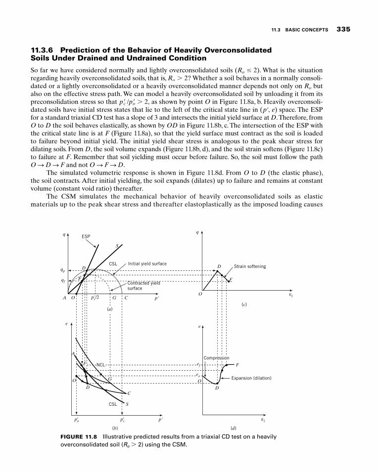
So far we have considered normally and lightly overconsolidated soils (Ro # 2). What is the situation regarding heavily overconsolidated soils, that is, Ro . 2? Whether a soil behaves in a normally consoli-dated or a lightly overconsolidated or a heavily overconsolidated manner depends not only on Ro but also on the effective stress path. We can model a heavily overconsolidated soil by unloading it from its preconsolidation stress so that p rc /p ro . 2, as shown by point O in Figure 11.8a, b. Heavily overconsoli-dated soils have initial stress states that lie to the left of the critical state line in (p9, e) space. The ESP for a standard triaxial CD test has a slope of 3 and intersects the initial yield surface at D. Therefore, from O to D the soil behaves elastically, as shown by OD in Figure 11.8b, c. The intersection of the ESP with the critical state line is at F (Figure 11.8a), so that the yield surface must contract as the soil is loaded to failure beyond initial yield. The initial yield shear stress is analogous to the peak shear stress for dilating soils. From D, the soil volume expands (Figure 11.8b, d), and the soil strain softens (Figure 11.8c) to failure at F. Remember that soil yielding must occur before failure. So, the soil must follow the path O S D S F and not O S F S D.

The simulated volumetric response is shown in Figure 11.8d. From O to D (the elastic phase), the soil contracts. After initial yielding, the soil expands (dilates) up to failure and remains at constant volume (constant void ratio) thereafter.

The CSM simulates the mechanical behavior of heavily overconsolidated soils as elastic materials up to the peak shear stress and thereafter elastoplastically as the imposed loading causes

FIGURE 11.8 Illustrative predicted results from a triaxial CD test on a heavily overconsolidated soil (Ro . 2) using the CSM.

CSL Initial yield surface

ESP

Strain softening

Contracted yieldsurface

S

D

F

O CG

O

D

A

C

G

S

O

O

D

F

F

D

p'

p'p'cp'o

ee

1

q q

qp

qf

A

(a)

(b)

(c)

(d)

1

CSL

ef

eo

Compression

Expansion (dilation)

ε

ε

F NCL

p'c/2


the soil to strain-soften toward the critical state line. In reality, heavily overconsolidated soils may behave elastoplastically before the peak shear stress is achieved, but this behavior is not captured by the simple CSM described here.

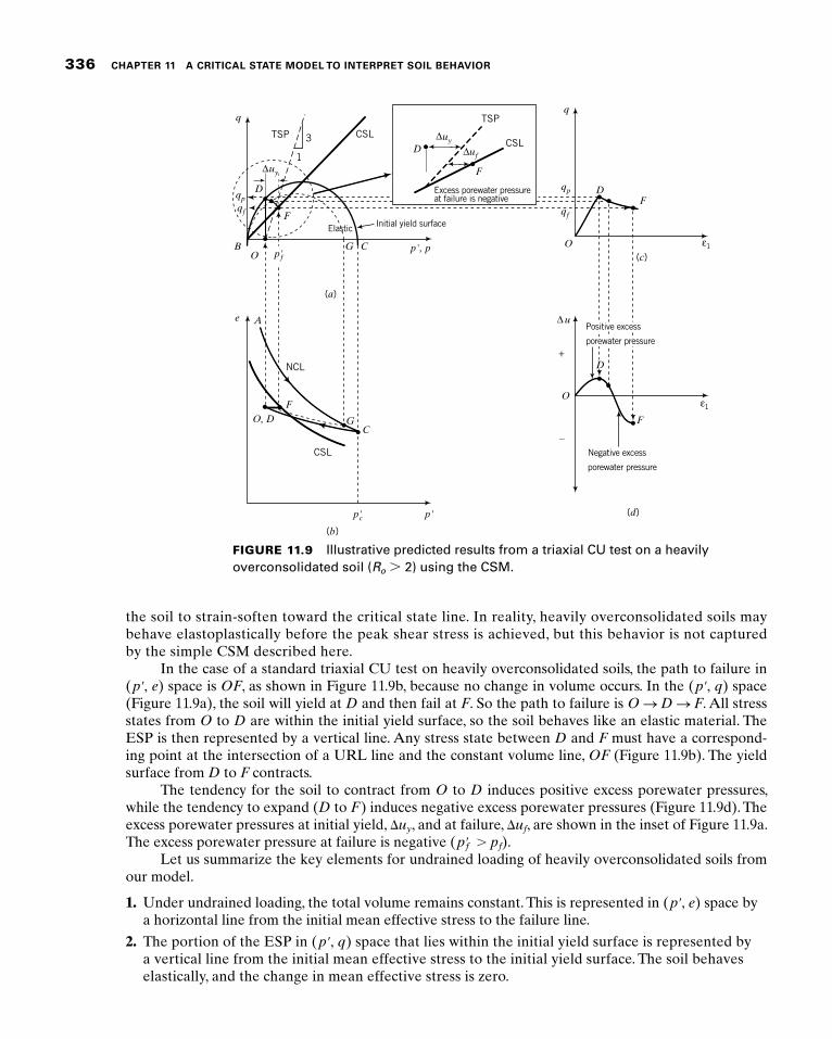
In the case of a standard triaxial CU test on heavily overconsolidated soils, the path to failure in (p9, e) space is OF, as shown in Figure 11.9b, because no change in volume occurs. In the (p9, q) space (Figure 11.9a), the soil will yield at D and then fail at F. So the path to failure is O S D S F. All stress states from O to D are within the initial yield surface, so the soil behaves like an elastic material. The ESP is then represented by a vertical line. Any stress state between D and F must have a correspond-ing point at the intersection of a URL line and the constant volume line, OF (Figure 11.9b). The yield surface from D to F contracts.

The tendency for the soil to contract from O to D induces positive excess porewater pressures, while the tendency to expand (D to F) induces negative excess porewater pressures (Figure 11.9d). The excess porewater pressures at initial yield, Duy, and at failure, Duf, are shown in the inset of Figure 11.9a. The excess porewater pressure at failure is negative (p9f . pf).

Let us summarize the key elements for undrained loading of heavily overconsolidated soils from our model.

1. Under undrained loading, the total volume remains constant. This is represented in (p9, e) space by a horizontal line from the initial mean effective stress to the failure line.

2. The portion of the ESP in (p9, q) space that lies within the initial yield surface is represented by a vertical line from the initial mean effective stress to the initial yield surface. The soil behaves elastically, and the change in mean effective stress is zero.

FIGURE 11.9 Illustrative predicted results from a triaxial CU test on a heavily overconsolidated soil (Ro . 2) using the CSM.

TSP

TSPCSL

CSL

CSL

NCL

D D

O, D

D

F

F

CG

F

F

F

OCG

A

B O

qq

qp

qp

qf qf

uy

u

1

1

uy

uf

Excess porewater pressure

Elastic Initial yield surface

at failure is negative

Negative excess

porewater pressure

3

1

(a)

(b)

(d)

p', p

p'p'c

e

+

–

O

(c)p'f

∆

∆

∆∆

ε

ε

Positive excess

porewater pressure

D


3. After initial yield, the soil may strain-soften (the initial yield surface contracts) or may strain-harden (the initial yield surface expands) to the critical state.

4. During elastic deformation under drained condition, the soil volume decreases (contracts), and after initial yield the soil volume increases (expands) to the critical state and does not change volume thereafter.

5. During elastic deformation under undrained condition, the soil develops positive excess porewater pressures, and after initial yield the soil develops negative excess porewater pressures up to the critical state. Thereafter, the excess porewater pressure remains constant.

6. The response of the soil under undrained condition is independent of the total stress path.

11.3.7 Prediction of the Behavior of Coarse-Grained Soils Using CSM

CSM is applicable to all soils. However, there are some issues about coarse-grained soils that require special considerations. Laboratory test data show that the NCL and CSL lines for coarse-grained soils are not well defi ned as straight lines in (ln p9, e) space (Figure 11.10) compared to those for fi ne-grained soils. The particulate nature of coarse-grained soils with respect to shape, size, roughness, structural arrangement (packing), particle hardness, and stiffness often leads to localized disconti-nuities. Tests using X rays on coarse-grained soils show shear banding (Figure 10.4) and nonuniform distribution of strains, even at low strains (,1%). Averaged stresses and strains normally deduced from measurements in soil test equipment cannot be relied upon to validate CSM. CSM is based on treating soils as continua, with smooth changes in stresses and strains. CSM cannot be used when shear bands occur. Other models (e.g., Coulomb or Mohr–Coulomb) may be more appropriate than CSM. However, the soil within the shear band is generally at critical state, and it is likely to behave as a viscous fl uid.

FIGURE 11.10 Illustrative volumetric responses of coarse-grained soils. p' (In scale)

NCL (dense sand)

Range of CSL

NCL (loose sand)e

Overconsolidation ratio and preconsolidation ratio are useful strictly for fi ne-grained soils. There is no standard technique to determine the preconsolidation stress for coarse-grained soils. There have been attempts to defi ne a new state parameter for coarse-grained soils within the CSM framework, with some success. These attempts are beyond the scope of this textbook. Despite the nonlinearity of the NCL and the CSL in (ln p9, e) space for coarse-grained soils, and the diffi culties in determining Ro or OCR, the framework by which CSM describes and integrates strength and deformation is still outstanding for all soils.

11.3.8 Critical State Boundary

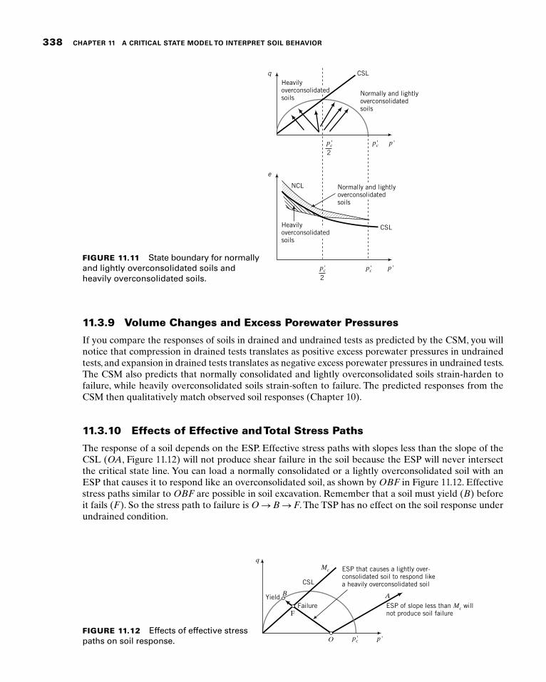
The CSL serves as a boundary separating normally consolidated and lightly overconsolidated soils from heavily overconsolidated soils (Figure 11.11). Stress states that lie to the right of the CSL will result in compression and strain-hardening of the soil; stress states that lie to the left of the CSL will result in expansion and strain-softening of the soil. More detailed analysis of how a soil will likely behave is given in Section 11.7.


11.3.9 Volume Changes and Excess Porewater Pressures

If you compare the responses of soils in drained and undrained tests as predicted by the CSM, you will notice that compression in drained tests translates as positive excess porewater pressures in undrained tests, and expansion in drained tests translates as negative excess porewater pressures in undrained tests. The CSM also predicts that normally consolidated and lightly overconsolidated soils strain-harden to failure, while heavily overconsolidated soils strain-soften to failure. The predicted responses from the CSM then qualitatively match observed soil responses (Chapter 10).

11.3.10 Effects of Effective and Total Stress Paths

The response of a soil depends on the ESP. Effective stress paths with slopes less than the slope of the CSL (OA, Figure 11.12) will not produce shear failure in the soil because the ESP will never intersect the critical state line. You can load a normally consolidated or a lightly overconsolidated soil with an ESP that causes it to respond like an overconsolidated soil, as shown by OBF in Figure 11.12. Effective stress paths similar to OBF are possible in soil excavation. Remember that a soil must yield (B) before it fails (F). So the stress path to failure is O S B S F. The TSP has no effect on the soil response under undrained condition.

FIGURE 11.11 State boundary for normally and lightly overconsolidated soils and heavily overconsolidated soils.

CSL

CSL

NCL

2

Normally and lightlyoverconsolidatedsoils

q

e

Heavilyoverconsolidatedsoils

Heavilyoverconsolidatedsoils

Normally and lightlyoverconsolidatedsoils

p'c p'c p'

2

p'c p'c p'

FIGURE 11.12 Effects of effective stress paths on soil response.

ESP that causes a lightly overconsolidated soil to respond like a heavily overconsolidated soil

B

F

q

O

FailureYield

CSL

Mc

p'

A

ESP of slope less than Mc willnot produce soil failure

p'c

11.4 ELEMENTS OF THE CRITICAL STATE MODEL 339

THE ESSENTIAL POINTS ARE: 1. There is a unique critical state line in (p9, q) space and a corresponding critical state line in (p9, e)

space for a soil.

2. There is an initial yield surface whose size depends on the preconsolidation mean effective stress.

3. The soil will behave elastically for stresses that are within the yield surface and elastoplastically for stresses directed outside the yield surface.

4. The yield surface expands for normally and lightly overconsolidated soils and contracts for heavily overconsolidated soils when the applied effective stresses exceed the initial yield stress.

5. The initial stress state of normally consolidated soils, Ro 5 1, lies on the initial surface.

6. Every stress state must lie on an expanded or contracted yield surface and on a corresponding URL.

7. Failure occurs when the ESP intersects the CSL and the change in volume is zero.

8. A soil must yield before it fails.

9. The excess porewater pressure is the difference in mean stress between the TSP and the ESP at a desired value of deviatoric stress.

10. The critical state model qualitatively captures the essential features of soil responses under drained and undrained loading.

What’s next . . . You were given an illustration using projection geometry of the essential ingredients of the critical state model. There were many unknowns. For example, you did not know the slope of the criti-cal state line and the equation of the yield surface. In the next section we will develop equations to fi nd these unknowns. Remember that our intention is to build a simple mosaic coupling the essential features of consolidation and shear strength.

11.4 ELEMENTS OF THE CRITICAL STATE MODEL

11.4.1 Yield Surface

The equation for the yield surface is an ellipse given by

1p r 2 2 2 p rprc 1q2

M2 5 0 (11.4a)

We can rewrite Equation (11.4a) as

q2 5 M 2pr 1prc 2 pr 2 (11.4b)

or

q 5 6M"p r 1p rc 2 p r 2 (11.4c)

or

q 5 6Mp rÅap rcp r

2 1b (11.4d)

or

p rc 5 pr 1q2

M2pr (11.4e)


The theoretical basis for the yield surface is presented by Schofi eld and Wroth (1968) and Roscoe and Burland (1968). You can draw the initial yield surface from the initial stresses on the soil if you know the values of M and p9c.

EXAMPLE 11.2 Plotting the Initial Yield Surface

A clay soil was consolidated to a mean effective stress of 250 kPa. If M 5 Mc 5 0.94, plot the yield surface.

Strategy For values of p9 from 0 to p9c, fi nd the corresponding values of q using Equation (11.4d). Then plot the results.

Solution 11.2

Step 1: Solve for q using values of p9 from 0 to p9c.

You can set up a spreadsheet to solve for q using various values of p9 from 0 to p9c 5 250 kPa, or you can use your calculator. For example, putting p9 5 100 kPa in Equation (11.4d) gives

q 5 60.94 3 100 c 250100

2 1 d12

5 6115.1 kPa

Step 2: Plot initial yield surface.

See Figure E11.2 (only the top half of the ellipse is shown).

FIGURE E11.2 p' (kPa)

3002001005000

40

100

80

20

60

140

120

150 250

q (k

Pa)

11.4.2 Critical State Parameters

11.4.2.1 Failure Line in (p9, q) Space The failure line in 1p r, q 2 space is

qf 5 Mp rf (11.5)

where qf is the deviatoric stress at failure, M is a frictional constant, and p9f is the mean effective stress at failure. By default, the subscript f denotes failure and is synonymous with critical state. For compression, M 5 Mc, and for extension, M 5 Me. The critical state line intersects the yield surface at p9c/2.


We can build a convenient relationship between M and f9cs for axisymmetric compression and extension and plane strain conditions as follows.

Axisymmetric Compression

Mc 5qf

p rf5

1s r1 2 s r3 2 fas r1 1 2s r3

3b

f

5

3as r1s r3

2 1bf

as r1s r3

1 2bf

We know from Chapter 10 that

as r1s r3b

f5

1 1 sin frcs

1 2 sin frcs

Therefore,

Mc 56 sin frcs

3 2 sin frcs (11.6)

or

sin frcs 53Mc

6 1 Mc (11.7)

Axisymmetric Extension In an axisymmetric (triaxial) extension, the radial stress is the major principal stress. Since in axial symmetry the radial stress is equal to the circumferential stress, we get

p rf 5 a2s r1 1 s r33

bf

qf 5 1s r1 2 s r3 2 fand

Me 5qf

p rf5

a2

s r1s r3

1 1bf

as r1s r3

2 1bf

56 sin frcs

3 1 sin frcs (11.8)

or

sin f rcs 53Me

6 2 Me (11.9)

An important point to note is that while the friction angle, f9cs, is the same for compression and exten-sion, the slope of the critical state line in (p9, q) space is not the same (Figure 11.13). Therefore, the fail-ure deviatoric stresses in compression and extension are different. Since Me , Mc, the failure deviatoric stress of a soil in extension is lower than that for the same soil in compression.


Plane Strain In plane strain, one of the strains is zero. In Chapter 7, we selected ε2 5 0; thus, s r2 2 0. In general, we do not know the value of s r2 unless we have special research equipment to mea-sure it. If s r2 5 C 1s r1 1 s r3 2 , where C 5 0.5, then

M 5 Mps 5 "3 sin frcs (11.10)

Taking C 5 0.5 presumes zero elastic compressibility. The subscript ps denotes plane strain. The constant, C, using a specially designed simple shear device (Budhu, 1984) on a sand, was shown to be approximately 12

tan f9cs. As an exercise, you can derive Equation (11.10) by following the derivation of Mc, but with p9

and q defi ned, as given by Equations (8.1) and (8.2).

11.4.2.2 Failure Line in (p9, e) Space Let us now fi nd the equation for the critical state line in (p9, e) space. We will use the (ln p9, e) plot, as shown in Figure 11.14c. The CSL is parallel to the nor-mal consolidation line and is represented by

ef 5 eG 2 l ln p rf (11.11)

where eG is the void ratio on the critical state line when p9 5 1 (G is the Greek uppercase letter gamma). This value of void ratio serves as an anchor for the CSL in (p9, e) space and (ln p9, e) space. The value of eG depends on the units chosen for the p9 scale. In this book, we will use kPa for the units of p9.

We will now determine eG from the initial state of the soil. Let us isotropically consolidate a soil to a mean effective stress p9c, and then isotropically unload it to a mean effective stress p9o (Figure 11.14a, b). Let X be the intersection of the unloading/reloading line with the critical state line. The mean effective stress at X is p9c/2, and from the unloading/reloading line,

eX 5 eo 1 k ln

proprc/2

(11.12)

where eo is the initial void ratio. From the critical state line,

eX 5 eG 2 l ln

prc2

(11.13)

Therefore, combining Equations (11.12) and (11.13), we get

eG 5 eo 1 1l 2 k 2 ln

prc2

1 k ln p ro (11.14)

FIGURE 11.13 Variation of the frictional constant M with critical state friction angle. φ'cs

353025200

0.4

1

0.8

0.2

0.6

1.6

1.2

1.4

MMe (extension)

Mc (compression)


THE ESSENTIAL CRITICAL STATE PARAMETERS ARE:l—Compression index, which is obtained from an isotropic or a one-dimensional consolidation test.

k—Unloading/reloading index or recompression index, which is obtained from an isotropic or a one-dimensional consolidation test.

M—Critical state frictional constant.

To use the critical state model, you must also know the initial stresses, for example, p9, eo, and p9c, and the initial void ratio, eo.

EXAMPLE 11.3 Calculation of M and Failure Stresses in Extension

A standard triaxial CD test at a constant cell pressure, s3 5 s93 5 120 kPa, was conducted on a sample of normally consolidated clay. At failure, q 5 s r1 2 s r3 5 140 kPa.

(a) Calculate Mc.

(b) Calculate p9f.

(c) Determine the deviatoric stresses at failure if an extension test were to be carried out so that failure occurs at the same mean effective stress.

Strategy You are given the fi nal stresses, so you have to use these to compute f9cs and then use Equation (11.6) to calculate Mc and Equation (11.8) to calculate Me. You can then calculate qf for the extension test by proportionality.

FIGURE 11.14 Void ratio, eG, to anchor critical state line.

CSL

e

e

O

e

q

eXeo

(c)(b)

(a)

1 p' (In scale)p'

p'

–––2

XX

CSL

CSL

Mc

p'c

p'c

–––2p'c

p'cp'o –––2p'c p'cp'o

λλ

κ

Γ


Solution 11.3

Step 1: Find the major principal stress at failure.

1s r1 2f 5 1s r1 2 s r3 2 1 s r3 5 140 1 120 5 260 kPa

Step 2: Find p9f .

p rf 5 as r1 1 2s r33

bf

5260 1 2 3 120

35 166.7 kPa

Step 3: Find f9cs.

sin f rcs 5s r1 2 s r3s r1 1 s r3

5140

260 1 1205 0.37

frcs 5 21.6°

Step 4: Find Mc and Me.

Mc 56 sin frcs

3 2 sin frcs5

6 3 0.373 2 0.37

5 0.84

Me 56 sin frcs

3 1 sin frcs5

6 3 0.373 1 0.37

5 0.66

Step 5: Find qf for extension.

qf 50.660.84

3 140 5 110 kPa; p rf 5qf

Me5

1100.66

5 166.7 kPa

EXAMPLE 11.4 Determination of l, k, and eG

A saturated soil sample is isotropically consolidated in a triaxial apparatus, and a selected set of data is shown in the table. Determine l, k, and eG.

Condition Cell pressure (kPa) Final void ratio

Loading 200 1.72 1000 1.20Unloading 500 1.25

Strategy Make a sketch of the results in (ln p9, e) space to provide a visual aid for solving this problem.

Solution 11.4

Step 1: Make a plot of ln p9 versus e.

See Figure E11.4.

Step 2: Calculate l.

From Figure E11.4,

l 5 2De

ln 1p rc 2 2 ln 1p r1 2 5 21.20 2 1.726.91 2 5.3

5 0.32

11.5 FAILURE STRESSES FROM THE CRITICAL STATE MODEL 345

Note: Figure E.11.4 is not a semilog (base e) plot. The abscissa is ln p9. If the data were plotted on a semilog (base e) plot, then

l 5 2De

ln 1p rc /p r1 2 5 21.20 2 1.72

ln a1000200

b5 0.32

Step 3: Calculate k.

From Figure E11.4,

k 5 2De

ln 1prc 2 2 ln 1pro 2 5 21.20 2 1.256.91 2 6.21

5 0.07

Step 4: Calculate eG.

eG 5 eo 1 1l 2 k 2 ln

prc2

1 k ln pro

5 1.25 1 10.32 2 0.07 2 ln

10002

1 0.07 ln 500 5 3.24

What’s next . . . We now know the key parameters to use in the CSM. Next, we will use the CSM to predict the shear strength of soils.

11.5 FAILURE STRESSES FROM THECRITICAL STATE MODEL

11.5.1 Drained Triaxial Test

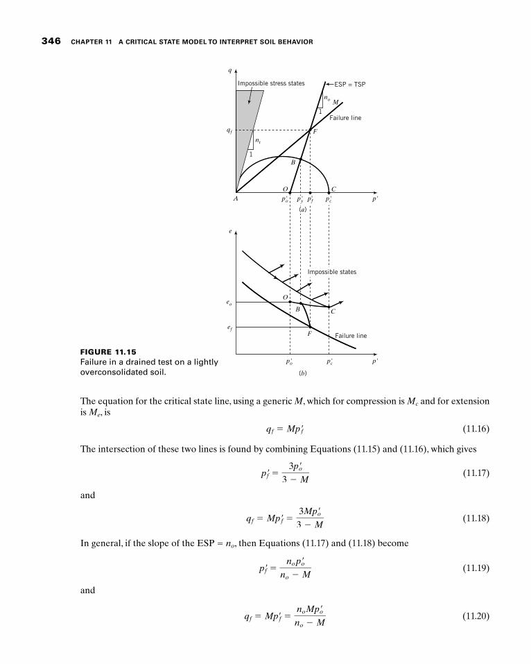
Let us consider a standard triaxial CD test in which we isotropically consolidate a soil to a mean effec-tive stress p9c and unload it isotropically to a mean effective stress of p9o (Figure 11.15a) such that Ro # 2. The slope of the ESP 5 TSP is 3, as shown by OF in Figure 11.15a. The ESP will intersect the critical state line at F. We need to fi nd the stresses at F. The equation for the ESP is

qf 5 3 1p rf 2 pro 2 (11.15)

FIGURE E11.4

76541.1

1.3

1.6

1.5

1.2

1.4

1.8

1.7

Void

rat

io

p1

λ = 0.32

κ = 0.07

p'cp'o

ln p''


The equation for the critical state line, using a generic M, which for compression is Mc and for extension is Me, is

qf 5 Mp rf (11.16)

The intersection of these two lines is found by combining Equations (11.15) and (11.16), which gives

p rf 53p ro

3 2 M (11.17)

and

qf 5 Mp rf 53Mp ro

3 2 M (11.18)

In general, if the slope of the ESP 5 no, then Equations (11.17) and (11.18) become

p rf 5nop ro

no 2 M (11.19)

and

qf 5 Mprf 5noMp rono 2 M

(11.20)

Impossible states

q

qf

e

eo

nt

no

ef

Impossible stress states

(a)

(b)

AO C

O

C

B

B

F

F

M

p'o p'y p'f p'c p'

p'p'cp'o

1

1Failure line

Failure line

ESP = TSP

FIGURE 11.15Failure in a drained test on a lightly overconsolidated soil.


Let us examine Equations (11.19) and (11.20). If M 5 Mc 5 no, then p9f → ` and qf → `. Therefore, Mc cannot have a value of no because soils cannot have infi nite strength. If Mc . no, then p9f is negative and qf is negative. Of course, p9f cannot be negative because soil cannot sustain tension. Therefore, we cannot have a value of Mc greater than no. Therefore, the region bounded by a slope q/p9 5 no originating from the origin and the deviatoric stress axis represents impossible soil states (Figure 11.15a). We will call this line the tension line. For standard triaxial tests, no 5 nt 5 3, where nt is the slope of the tension

line. For extension triaxial tests, the slope of the tension line is nt 5 232

. In the case of plane strain tests,

if tension is parallel to the minor principal effective stress 1s3r 2 and s r2 5 0.5 1s r1 1 s r3 2 , then the slope of the tension line nt 5 !3. (You should prove this as an exercise.)

Also, you should recall from Chapter 9 that soil states to the right of the normal consolidation line are impossible (Figure 11.15b). We have now delineated regions in stress space (p9, q) and in void ratio versus mean effective stress space—that is, (p9, e) space—that are possible for soils. Soil states cannot exist outside these regions.

For overconsolidated soil, the initial yield stress is attained when the ESP intersects the initial yieldsurface, point B in Figure 11.15a. The coordinate for the yield stresses is found by setting q 5 qy 5 no 1p ry 2 p ro 2 and p9 5 p9y. Thus,

no(pry 2 pro) 5 6Mp ry Åaprcpry

2 1b (11.21)

Solving for p9y gives

pry 5 prp 51M2p rc 1 2n2

o pro 2 1 "1M2prc 1 2n2o pro 2 2 2 4n2

o 1M2 1 n2o 2 1pro 2 2

2 1M2 1 n2o 2 (11.22)

Dividing the numerator on the right-hand side of Equation (11.22) by p9o gives

p ry 5

proC aM2

prcpro

1 2n2ob 1 ÅaM2

p rcpro

1 2n2ob

2

2 4n2o 1M2 1 n2

o 2 S2 1M2 1 n2

o 2 5

proS 1M2Ro 1 2n2o 2 1 "1M2Ro 1 2n2

o 2 2 2 4n2o 1M2 1 n2

o 2 T2 1M2 1 n2

o 2 (11.23)

The yield shear stress is

ty 5qy

25

no 1p ry 2 p ro 22

(11.24)

For the standard triaxial test, no 5 3.

11.5.2 Undrained Triaxial Test

In an undrained test, the total volume change is zero. That is, DV 5 0 or Dεp 5 0 or De 5 0 (Figure 11.16) and, consequently,

ef 5 eo 5 eG 2 l ln prf (11.25)


By rearranging Equation (11.25), we get

p rf 5 exp aeG 2 eo

lb (11.26)

Since qf 5 Mp9f, then

qf 5 M exp aeG 2 eo

lb (11.27)

Recall from Section 11.3.5 that the shear behavior of soils under undrained condition is indepen-dent of the total stress path. Equation (11.27) confi rms this, as it has no parameter that is related to the total stress path. The undrained shear strength, denoted by su, is defi ned as one-half the deviatoric stress at failure. That is,

1su 2 f 5qf

25

M2

exp aeG 2 eo

lb (11.28)

It is valid for normally consolidated, lightly overconsolidated, and heavily overconsolidated soils. For a given soil, M, l, and eG are constants and the only variable in Equation (11.28) is the initial void ratio. Therefore, the undrained shear strength of a particular saturated fi ne-grained soil depends only on the initial void ratio or initial water content. You should recall that we discussed this in Chapter 10 but did not show any mathematical proof. Also, su is not a fundamental soil property because it depends on the initial state of the soil.

CSL

ESPF

B

FF O, B

O C

C

A

uf

1

13

∆

TSP

p�f p�o

qy

eo = ef

qf

nt

e e

e

q

p�c p'

p' p' (In scale)

Impossible stress state

Impossible state

1

CSLCSL

NCL

O, B

Γ

NCL

FIGURE 11.16 Failure in an undrained test on a lightly overconsolidated soil.


We can use Equation (11.28) to compare the undrained shear strengths of two samples of the same soil tested at different void ratio, or to predict the undrained shear strength of one sample if we know the undrained shear strength of the other. Consider two samples, A and B, of the same soil. The ratio of their undrained shear strength is

1su 2A1su 2B 5

cexp aeG 2 eo

lb d

A

cexp aeG 2 eo

lb d

B

5 exp a 1eo 2B 2 1eo 2Al

b

For a saturated soil, eo 5 wGs and we can then rewrite the above equation as

1su 2A1su 2B 5 exp cGs 1wB 2 wA 2

ld (11.29)

Let us examine the difference in undrained shear strength for a 1% difference in water content between samples A and B. We will assume that the water content of sample B is greater than that of sample A, that is, (wB 2 wA) is positive, l 5 0.15 (a typical value for a silty clay), and Gs 5 2.7. Putting these values into Equation (11.29), we get

1su 2A1su 2B 5 1.20

That is, a 1% increase in water content causes a reduction in undrained shear strength of 20% for this soil. The implication for soil testing is that you should preserve the water content of soil samples, espe-cially samples taken from the fi eld, because the undrained shear strength can be signifi cantly altered by even small changes in water content.

The ESP is vertical 1Dp r 5 0 2 within the initial yield surface, and after the soil yields, the ESP bends toward the critical state line, as the excess porewater pressure increases considerably after yield. The excess porewater pressure at failure is found from the difference between the mean total stress and the corresponding mean effective stress at failure. It consists of two components. One component, called the shear component, Dus

f (Figure 11.17, FA), is related to the shearing behavior. The other component, called the total stress component, Dut

f (Figure 11.17, AB), is connected not to the shearing behavior but to the total stress path. If two samples of the same soil at the same initial stress state are subjected to two different TSP, say, OT and OR in Figure 11.17, the shear component of the excess porewater pressure would be the same, but the total stress path component would be different (compare AB and AD in Figure 11.17). The total excess porewater pressure at failure (critical state) is

Duf 5 Dusf 1 Dut

f 5 1p ro 2 p rf 2 1qf

no (11.30)

FIGURE 11.17Excess porewater pressuresduring undrained loading.

q

qf

TS

R

DB

F

O

A

p'f p'o

∆uft

∆uf = ∆ufs + ∆uf

t

∆ufs

TSPCSL

1

qf

no

no


Substituting qf 5 Mp rf in Equation (11.30), we get

Duf 5 p ro 2 p rf 1Mp rfno

5 p ro 1 p rf aMno

2 1b (11.31)

By substituting Equation (11.26) into Equation (11.31), we obtain

Duf 5 pro 1 aMno

2 1b exp aeG 2 eo

lb (11.32)

For a standard triaxial CU test, no 5 3, and

Duf 5 p ro 1 aM3

2 1b exp aeG 2 eo

lb (11.33)

The right-hand side of Equation (11.28) can be transformed into mean effective stress terms by substituting Equation (11.14) and carrying out algebraic manipulations. However, we will use a more elegant mathematical method (Wroth, 1984). We start by defi ning an equivalent stress originally pro-posed by Hvorslev (1937). The equivalent effective stress is the mean effective stress on the NCL that has the same void ratio as the current mean effective stress. With reference to Figure 11.18, the equiva-lent effective stress for point O on the URL is p ra.

Let us consider two samples of the same soil. One of them, sample I, is normally consolidated to C in Figure 11.18, i.e., Ro 5 1. The other, sample II, is normally consolidated to C and then unloaded to O. That is, sample II is heavily overconsolidated, with Ro greater than 2. The intersection of the CSL

with the URL is at X and the mean effective stress is prc2

. Both samples are to be loaded to failure

under undrained condition. Sample I will fail at D on the CSL, while sample II will fail at F on the CSL. The equivalent effective stress for sample I is p rc, while for sample II it is p ra. Note that sampleI is on both the NCL and the URL. The change in void ratio from A to C on the NCL is

ea 2 ec 5 l ln

p rcp ra

(11.34)

The change in void ratio from O to C on the URL is

eo 2 ec 5 k ln

prcpro

5 k ln Ro (11.35)

Now ea 5 eo, and thus

l ln p rcp ra

5 k ln Ro (11.36)

URL

NCL

CSL

e

eo = ea = ef

ed = ec

O FX

A

DC

p'o p'f p'd p'a p'c p' (In scale)

λ

λ

κ

FIGURE 11.18Normal consolidation, unloading/reloading, and critical state lines in (p9, e) space.


Points F and X are on the CSL. By similar triangles (FOX and AOC), we get

l ln prxp rf

5 k ln prxpro

(11.37)

By subtracting both sides of Equation (11.37) from l ln prxpro

, we get

l ln

prxpro

2 l ln

prxprf

5 l ln

prxp ro

2 k ln prxpro

(11.38)

which simplifi es to

l ln

p rfp ro

5 1l 2 k 2 ln

p rxp ro

(11.39)

Substituting prx 5prc2

and Ro 5prcpro

into Equation (11.39) gives

l ln

p rfpro

5 1l 2 k 2 ln

p rc2

pro5 1l 2 k 2 ln aRo

2b (11.40)

Simplifying Equation (11.40) gives

prfpro

5 aRo

2bL

(11.41)

where L 5l 2 k

l5 1 2

k

l5

Cc 2 Cr

Cc5 1 2

Cr

Cc is the plastic volumetric strain ratio (Schofi eld and

Wroth, 1968); L is Greek uppercase letter lambda. An approximate value for L is 0.8. The undrained shear strength at the critical state is then

1su 2 f 5qf

25

Mp rf2

5Mp ro

2 aRo

2bL

(11.42)

Equation (11.28) and Equation (11.42) will predict the same value of undrained shear strength at the critical state. These equations are just representations of the undrained shear strength with different parameters. Equation (11.28) is advantageous if the water content is known.

Heavily overconsolidated fi ne-grained or dense-to-medium-dense coarse-grained soils may exhibit a peak shear stress and then strain-soften to the critical state (Figure 11.9). However, the attainment of a peak stress depends on the initial stress state and the ESP. Recall that according to CSM, soils would behave elastically up to the initial yield stress (peak deviatoric stress), qy. By substituting p9 5 p9o and q 5 qy in the equation for the yield surface [Equation (11.4d)], we obtain

qy 5 Mp roÅprcpro

2 1 5 Mpro"Ro 2 1; Ro . 1 (11.43)

The undrained shear strength for fi ne-grained soils at initial yield is

1su 2 y 5M2

pro"Ro 2 1; Ro . 1 (11.44)

We will discuss the implications of Equation (11.44) for the design of geosystems in Section 11.7.


THE ESSENTIAL POINTS ARE:1. The intersection of the ESP and the critical state line gives the failure stresses.

2. The undrained shear strength depends only on the initial void ratio.

3. Small changes in water content can signifi cantly alter the undrained shear strength.

4. The undrained shear strength is independent of the total stress path.

EXAMPLE 11.5 Predicting Yield Stresses for Drained ConditionA clay sample was isotropically consolidated under a cell pressure of 250 kPa in a triaxial test and then unloaded isotropically to a mean effective stress of 100 kPa. A standard CD test is to be conducted on the clay sample by keeping the cell pressure constant and increasing the axial stress. Predict the yield stresses, p9y and qy, if M 5 0.94.

Strategy This is a standard triaxial CD test. The ESP has a slope no 5 3. The yield stresses can be found from the intersection of the ESP and the initial yield surface. The initial yield surface is known, since p9c 5 250 kPa and M 5 0.94.

Solution 11.5

Step 1: Make a sketch or draw a scaled plot of the initial yield surface.

1p r 2 2 2 250 p rc 1q2

y

10.94 2 2 5 0

The yield surface is the same as in Example 11.2. See Figure E11.5.

p' (kPa)

3002001005000

40

100

80

20

60

160

140

120

150

1

3

ESP

250

q (k

Pa)

B

Initial yield

FIGURE E11.5

Step 2: Find the equation for the ESP.

The equation for the ESP is

p r 5 p ro 1q

3

See Figure E11.5.

Step 3: Find the intersection of the ESP with the initial yield surface.

Let B 5 (p9y, qy) be the yield stresses at the intersection of the initial yield surface with the ESP (Figure E11.5). At B, the equation for the yield surface is

1p ry 2 2 2 250 pry 1q2

y

10.94 2 2 5 0 (1)


At B, the equation for the ESP is

pry 5 pro 1qy

3 (2)

Inserting Equation (2) into Equation (1), we can solve for qy as follows:

apro 1qy

3b2

2 250 apro 1qy

3b 1

q2y

10.94 2 2 5 0

5 a100 1qy

3b2

2 250 a100 1qy

3b 1

q2y

10.94 2 2 5 0

The solution gives qy 5 117 kPa and 2103.5 kPa. Since the test is compression, the correct solution is qy 5 117 kPa (see Figure E11.5).

Solving for p9y from Equation (2) gives

p ry 5 p ro 1qy

35 100 1

1173

5 139 kPa

You can also use Equation (11.23). Try this for yourself.

EXAMPLE 11.6 Predicting Yield Stresses for Undrained ConditionRepeat Example 11.5, except that the clay was sheared under undrained condition. In addition, calculate the excess porewater pressure at initial yield.

Strategy In this case, the TSP has a slope no 5 3. Since the soil will behave elastically within the initial yield surface, the ESP is vertical (see Chapter 8). The yield stresses can be found from the intersection of the ESP and the initial yield surface.

Solution 11.6

Step 1: Identify given parameters.

pro 5 100 kPa, p rc 5 250 kPa, Ro 5prcpro

5250100

5 2.5

M 5 0.94

Step 2: Calculate yield stresses.

qy 5 Mp ro"Ro 2 1 5 0.94 3 100"2.5 2 1 5 115 kPa

p ry 5 p ro 5 100 kPa

See Figure E11.6.

FIGURE E11.6 p' (kPa)

3002001005000

40

100

80

20

60

160

140

120

150

1

3

TSP

ESP

250

q (k

Pa)

B


Step 3: Calculate the total mean stress at yield.

py 5 po 1qy

35 100 1

1153

5 138.3 kPa

Step 4: Calculate the excess porewater pressure at yield.

Duy 5 py 2 p ro 5 138.3 2 100 5 38.3 kPa

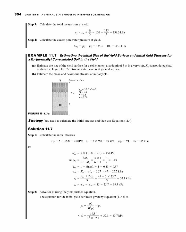
EXAMPLE 11.7 Estimating the Initial Size of the Yield Surface and Initial Yield Stresses for a Ko- (normally) Consolidated Soil in the Field

(a) Estimate the size of the yield surface for a soil element at a depth of 5 m in a very soft, Ko-consolidated clay, as shown in Figure E11.7a. Groundwater level is at ground surface.

(b) Estimate the mean and deviatoric stresses at initial yield.

γsat = 18.8 kN/m3

M = 1.0λ = 0.3κ = 0.06

Ground surface

5 m

FIGURE E11.7a

Strategy You need to calculate the initial stresses and then use Equation (11.4).

Solution 11.7

Step 1: Calculate the initial stresses.

szo 5 5 3 18.8 5 94 kPa; uo 5 5 3 9.8 5 49 kPa; s rzo 5 94 2 49 5 45 kPa

or

s rzo 5 5 3 118.8 2 9.8 2 5 45 kPa

sin fcs 53Mc

6 1 Mc5

3 3 16 1 1

537

5 0.43

Ko 5 1 2 sin frcs 5 1 2 0.43 5 0.57

s rxo 5 Ko 3 srzo 5 0.57 3 45 5 25.7 kPa

pro 5s rzo 1 2srxo

35

45 1 2 3 25.73

5 32.1 kPa

qo 5 s rzo 2 s rxo 5 45 2 25.7 5 19.3 kPa

Step 2: Solve for prc using the yield surface equation.

The equation for the initial yield surface is given by Equation (11.4e) as

p rc 5q2

o

M2pro1 pro

6 prc 519.32

12 3 32.11 32.1 5 43.7 kPa


Step 3: Estimate stresses at initial yield.

pry 5 pro 5 32.1 kPa; qy 5 qo 5 19.3 kPa

See Figure E11.7b for a plot of the initial yield surface and initial yield point, O.

FIGURE E11.7b

5040 4530 3510 15 20 25500

5

10

15

20

25

30

35

ESP

p' (kPa)

q (k

Pa)

Ko consolidation

O(32.1, 19.3)

Failure lineM = 1

Failure (23.6, 23.6)

EXAMPLE 11.8 Predicting Failure Stresses for a Ko- (normally) Consolidated Soil in the Field

(a) For the soil element in Example 11.7, what additional stresses, Dp9 and Dq, will cause it to fail under undrained condition?

(b) Predict the undrained shear strength.

Strategy You need to calculate the failure stresses for undrained loading. From the given data, calculate eo and eG, then fi nd the failure stresses. The additional stresses are the differences between the initial and failure stresses.

Solution 11.8

Step 1: Find eo and eG.

gsat 5 aGs 1 eo

1 1 eobgw

eo 5 ±Gs 2

gsat

gw

gsat

gw2 1

≤ 5 ±2.7 2

18.89.8

18.89.8

2 1≤ 5 0.84

eG 5 eo 1 1l 2 k 2 ln

p rc2

1 k ln p ro

5 0.84 1 10.3 2 0.06 2 ln 43.7

21 0.06 ln 132.1 2 5 1.788

Step 2: Find failure stresses.

p rf 5 exp aeG 2 eo

lb 5 exp a1.788 2 0.84

0.3b 5 23.6 kPa

Since qf 5 Mp9f, then qf 5 1 3 23.6 5 23.6 kPa. You will get the same result using Equation (11.41).

Step 3: Find increase in stresses to cause failure.

Dprf 5 p rf 2 p ro 5 23.6 2 32.1 5 28.5 kPa

Dqf 5 qf 2 qo 5 23.6 2 19.3 5 4.3 kPa

Note that there is no initial elastic state for a normally consolidated soil. See Figure E11.7b.


Step 4: Calculate the undrained shear strength.

1su 2 f 5qf

25

23.62

5 11.8 kPa

EXAMPLE 11.9 Predicting Yield and Failure Stresses and Excess Porewater PressuresTwo specimens, A and B, of a clay were each isotropically consolidated under a cell pressure of 300 kPa and then unloaded isotropically to a mean effective stress of 200 kPa. A CD test is to be conducted on specimen A and a CU test is to be conducted on specimen B.

(a) Estimate, for each specimen, (a) the yield stresses, p9y, qy, (s91)y, and (s93)y; and (b) the failure stresses p9f, qf, (s91)f, and (s93)f.

(b) Estimate for sample B the excess porewater pressure at yield and at failure.

The soil parameters are l 5 0.3, k 5 0.05, eo 5 1.10, and f9cs 5 308. The cell pressure was kept constant at 200 kPa.

Strategy Both specimens have the same consolidation history but are tested under different drainage condi-tions. The yield stresses can be found from the intersection of the ESP and the initial yield surface. The initial yield surface is known since p9c 5 300 kPa, and M can be found from f9cs. The failure stresses can be obtained from the intersection of the ESP and the critical state line. It is always a good habit to sketch the q versus p9 and the e versus p9 graphs to help you solve problems using the critical state model. You can also fi nd the yield and failure stresses using graphical methods, as described in the alternative solution.

Solution 11.9

Step 1: Calculate Mc.

Mc 56 sin 30°

3 2 sin 30°5 1.2

Step 2: Calculate eG.

With p9o 5 200 kPa and p9c 5 300 kPa,

eG 5 eo 1 1l 2 k 2 ln

p rc2

1 k ln p ro

5 1.10 1 10.3 2 0.05 2 ln 300

21 0.05 ln 200 5 2.62

Step 3: Make a sketch or draw scaled plots of q versus p9 and e versus p9.

See Figure E11.9a, b.

Step 4: Find the yield stresses.

Drained Test Let p9y and qy be the yield stress (point B in Figure E11.9a). From the equation for the yield surface [Equation (11.4d)],

qy 5 6Mp ryÅap rcp ry

2 1b 5 61.2p ryÅa300p ry

2 1b (1)

From the ESP,

qy 5 3 1p ry 2 p ro 2 5 3p ry 2 600 (2)


Solving Equations (1) and (2) for p9y and qy gives two solutions: p9y 5 140.1 kPa, qy 5 2179.6 kPa; and p9y 5 246.1 kPa, qy 5 138.2 kPa. Of course, qy 5 2179.6 kPa is not possible because we are conducting a compression test. The yield stresses are then p9y 5 246.1 kPa, qy 5 138.2 kPa.

Now,

qy 5 1s r1 2 y 2 1s r3 2 y 5 138.2 kPa; 1s r3 2 f 5 200 kPa

Solving for (s91)f gives

1s r1 2 f 5 138.2 1 200 5 338.2 kPa

Undrained Test The ESP for the undrained test is vertical for the region of stress paths below the yield stress, that is, Dp9 5 0. From the yield surface [Equation (11.4d)] for p9 5 p9y 5 p9o, we get

q 5 qy 5 6Mp roÅap rcp ro

2 1b 5 61.2 3 200Åa300200

2 1b 5 169.7 kPa

From the TSP, we can fi nd py (B9, Figure E11.9c):

py 5 p ro 1qy

35 200 1

169.73

5 256.6 kPa

The excess porewater pressure at yield is

Duy 5 py 2 p ry 5 py 2 pro 5 256.6 2 200 5 56.6 kPa

Now,

p ry 5 p ro 51s r1 2 y 1 2 1s r3 2 y

35 200 kPa

qy 5 1s r1 2 y 2 1s r3 2 y 5 169.7 kPa

5004003002001000

50040030020010000.5

1

1.5

2

2.5

0

100

200

300

400

500

B

BF

Initial yield surface

F CSL

CSL

p'y

qy

p'f

A C

A

C

O

p' (kPa)

p' (kPa)

q (k

Pa)

(a)

(b)

e

FIGURE E11.9a, b


Solving for (s91)y and (s93)y gives

1s r1 2 y 5 313.3 kPa; 1s r3 2 y 5 143.4 kPa

Check

1s3 2 y 5 1s r3 2 y 1 Duy 5 143.4 1 56.6 5 200 kPa

Step 5: Find the failure stresses.

Drained Test

Equation (11.17): p rf 53 3 2003 2 1.2

5 333.3 kPa

Equation (11.18): qf 5 1.2 3 333.3 5 400 kPa

Now,

qF 5 1s r1 2 f 2 1s r3 2 f 5 400 kPa and 1s r3 2 f 5 200 kPa

Solving for (s91)f, we get

1s r1 2 f 5 400 1 200 5 600 kPa

Undrained Test

L 5l 2 k

l5

0.3 2 0.050.3

5 0.833; Ro 5 300/200 5 1.5

p' (kPa)

50040030020010000

100

200

300

400

500

q (k

Pa)

(c)

(d)

ESP

TSP

CSLS

Initial yield surface

B'B

A C

F F'10557

qf

p'f

qy

p' (kPa)

50040030020010000.5

1

1.5

2

2.5

e

CSL F

AC

FIGURE E11.9c, d


Equation (11.41): p rf 5 p roaRo

2bL

5 200 a1.52b0.833

5 157 kPa

Equation (11.5): qf 5 1.2 3 157 5 188.4 kPa

Alternatively:

Equation (11.26): p rf 5 expa2.62 2 1.100.3

b 5 158.6 kPa

Equation (11.5): qf 5 1.2 3 158.6 5 190.3 kPa

The difference between the results of Equation (11.41) and Eq. (11.26) is due to rounding errors.

Now,

p rf 51s r1 2 f 1 2 1s r3 2 f

35 158.6 kPa

qf 5 1s r1 2 f 2 1s r3 2 f 5 190.4 kPa

Solving for (s91)f and (s93)f, we fi nd

1s r1 2 f 5 285.5 kPa and 1s r3 2 f 5 95.1 kPa

We can fi nd the excess porewater pressure at failure from either Equation (11.34),

Duf 5 200 1 a1.23

2 1bexpa2.62 2 1.100.3

b 5 104.9 kPa

or

Duf 5 s3 2 1s r3 2 f 5 200 2 95.1 5 104.9 kPa

Graphical Method We need to fi nd the equations for the normal consolidation line and the critical state lines.

Normal Consolidation Line Void ratio at preconsolidation stress:

ec 5 eo 2 k ln p rcp ro

5 1.10 2 0.05 ln 300200

5 1.08

Void ratio at p9 5 1 kPa on NCL:

en 5 ec 1 l ln p rc 5 1.08 1 0.3 ln 300 5 2.79

The equation for the normal consolidation line is then

e 5 2.79 2 0.3 ln p r

The equation for the unloading/reloading line is

e 5 1.08 1 0.05 ln p rcp r

The equation for the critical state line in (ln p9, e) space is

e 5 2.62 2 0.3 ln p r

Now you can plot the normal consolidation line, the unloading/reloading line, and the critical state line, as shown in Figure E11.9b.


Plot Initial Yield Surface The yield surface [Equation (11.4d)] is

q 5 61.2p rÅ300p r

2 1

For p9 5 0 to 300, plot the initial yield surface, as shown in Figure E11.9a.

Plot Critical State Line The critical state line is

q 5 1.2p r

and is plotted as OF in Figure E11.9a.

Drained Test The ESP for the drained test is

p r 5 200 1q

3

and is plotted as AF in Figure E11.9a. The ESP intersects the initial yield surface at B and the yield stresses are p9y 5 240 kPa and qy 5 138 kPa. The ESP intersects the critical state line at F, and the failure stresses are p9f 5 333 kPa and qf 5 400 kPa.

Undrained Test For the undrained test, the initial void ratio and the fi nal void ratio are equal. Draw a horizontal line from A to intersect the critical state line in (p9, e) space at F (Figure E11.9d). Project a vertical line from F to intersect the critical state line in (p9, q) space at F (Figure E11.9c). The failure stresses are p9f 5 159 kPa and qf 5 190 kPa. Draw the TSP, as shown by AS in Figure E11.16c. The ESP within the elastic region is vertical, as shown by AB. The yield stresses are p9y 5 200 kPa and qy 5 170 kPa. The excess porewater pressures are:

At yield—horizontal line BB9: Duy 5 57 kPa

At failure—horizontal line FF9: Duf 5 105 kPa

EXAMPLE 11.10 Predicting su in Compression and Extension Tests on a Heavily Overconsolidated ClayDetermine the undrained shear strength at initial yield in (a) a CU compression test and (b) a CU extension test for a clay soil with Ro 5 5, p9o 5 70 kPa, and f9cs 5 258.

Strategy Since you are given f9cs, you should use Equations 11.6 and 11.8 to fi nd Mc and Me. Use Equation (11.44) to solve the problem.

Solution 11.10

Step 1: Calculate Mc and Me.

Mc 56 sin f rcs

3 2 sin f rcs5

6 sin 25°3 2 sin 25°

5 0.98

Me 56 sin f rcs

3 1 sin f rcs5 0.74

Step 2: Calculate su.

Use Equation (11.44).

Compression: 1su 2 y 50.98

23 70"5 2 1 5 68.6 kPa

Extension: 1su 2 y 50.74

23 70"5 2 1 5 51.8 kPa

11.6 MODIFICATIONS OF CSM AND THEIR PRACTICAL IMPLICATIONS 361

Or, by proportion,

Extension: 1su 2 y 50.740.98

3 68.6 5 51.8 kPa

EXAMPLE 11.11 Effects of Change of Water Content on su

The in situ water content of a soil sample is 48%. The water content decreases to 44% due to transportation of the sample to the laboratory and during sample preparation. What difference in undrained shear strength could be expected if l 5 0.13 and Gs 5 2.7?

Strategy The solution to this problem is a straightforward application of Equation (11.29).

Solution 11.11

Step 1: Determine the difference in su values.

Use Equation (11.29).

1su 2 lab1su 2 field5 exp

3Gs 1wfield 2 wlab 2 4l

5 exp c 2.7 10.48 2 0.44 20.13

d 5 2.3

The laboratory undrained shear strength would probably show an increase over the in situ undrained shear strength by a factor greater than 2.

What’s next . . . In the next section, we consider some practical implications of the CSM.

11.6 MODIFICATIONS OF CSM AND THEIRPRACTICAL IMPLICATIONS

The CSM is the foundation of many popular soil models used in numerical analyses. CSM have been shown to be particularly good in simulations of normally and lightly overconsolidated fi ne-grained soils, but not as good for heavily overconsolidated clays and coarse-grained soils. Various modifi cations in the literature have been made to CSM so as to model more complex loading conditions than those described so far in this chapter and to better describe heavily overconsolidated clays and coarse-grained soils. We are going to make some simple modifi cations to CSM to improve its versatility in modeling a wide range of soil types and to establish some additional conceptual understanding of soil behavior.

We considered a particular shape of the yield surface in developing the concept of critical state model. Other shapes of yield surfaces have been developed and used in predicting soil responses. For example, Schofi eld and Wroth (1968) developed a bullet-shaped yield surface using energy methods. For heavily overconsolidated soils, the peak (initial yield) shear strength occurs on the initial yield surface, which in our case is an ellipse. Experimental data from shear box tests on heavily overconsolidated clays presented by Hvorslev (1937) reveal that the locus of peak shear strength is approximately a straight line. In considering heavily overconsolidated fi ne-grained soils, we will replace that portion of the initial elliptical yield surface on the left side of the critical state line by the straight line found by Hvorslev. This line defi nes limiting stress states and is not a yield surface.

In Figure 11.19a, b, AT, At, and ac are lines that separate possible from impossible states; ac is the normal consolidation line; AT and At delineate limiting tensile stress states labeled TL; AF and gf are the critical state or failure lines; TF is Hvorslev’s surface, labeled HV surface. Line ct is an unloading/reloading line.


The HV surface defi nes stress states at incipient instability and is fi xed in stress space. It lies

between p r 5prc2

and prt, where prt is mean effective stress at the intersection of the TL and the HV

surfaces. The surface FC is a yield surface and not a limiting stress surface. It is labeled RSW (after Roscoe, Schofi eld, and Wroth, 1958). Unlike the HV surface, the RSW surface is not fi xed in stress space. It can expand or contract. It is bounded by the critical state line and the mean effective stress axis [isotropic stress path in (p9, q) space]. Soil stress states on AT will cause the soil to fail in tension. Recall that uncemented soils cannot sustain tension.

We are going to describe three regions of soil behavior, as in Section 10.7.

Region I. Soil stress states within Region I are impossible. During unloading the soil cannot follow paths right of the normal consolidation line, ac (Figure 11.19b). Also, uncemented soils cannot have stress states left of the tension line, AT or At.

Region II. Soil stress states within Region II, area ATFA (Figure 11.19a), would cause the soil to behave elastically, but on approaching the HV surface it may exhibit discontinuous response and fail with one or more bifurcations. In laboratory shear tests, it has been observed that just prior to achieving the peak shear strength and during strain softening, preferential zones of dilation (shear bands, Figure 10.4) develop. Due to progressive softening, the size of these preferential zones of dilation increases during postpeak shear deformation.

The permeability or hydraulic conductivity of the soil (especially within the shear bands or pref-erential zones of dilation) increases and, if water is present, this increased permeability can lead to sudden failure due to seepage (for example, fl ow slides on a slope). The presence of preferential zones of dilation as the soil mass strain-softens renders CSM inadmissible because CSM treats soils as continua. Calculations using CSM in the strain-softening regime of soil behavior cannot be expected to be accurate.

Loads that bring the soil to stress states near or on the HV surface present a high safety risk.

Region III. Soil stress states within Region III (AFCA, Figure 11.19a) will cause the soil to behave in a ductile manner. It is desirable to design geotechnical systems such that the soil will behave in

CSL

CSLURL

NCL

2

Yield surfaceRSW

q

C

clf

e

Discontinuousresponse,brittleness

HVRegion I

Region II

Region III

Ductile,plasticyielding

p'cp't p'c p'

a

t

A

A

L

Fnt

TTL

Region I

Region I

Region II

1

2

p'cp't p'c

g

(a)

(b)

Region IIIDuctile responseFIGURE 11.19

Regional description and expected responses of soil.

11.6 MODIFICATIONS OF CSM AND THEIR PRACTICAL IMPLICATIONS 363

a ductile manner under anticipated loadings. Soil states on the CSL are failure states. Your design loads should not bring the soil state to failure under any anticipated loading condition.

Let us examine the behavior of three samples of the same soil in undrained triaxial tests. The fi rst, sample A, is lightly overconsolidated, 2 . Ro . 1. The second, sample B, is heavily overconsolidated,

Rt . Ro . 2, where Rt 5prcprt

. The third, sample C, is very heavily overconsolidated, Ro . Rt. The theoretical

response of the lightly overconsolidated soil is shown in Figure 11.20a. From O to A the soil behaves elastically [recall that the ESP for an elastic soil under undrained condition is vertical in (p9, q) space]. At A, the soil yields, and as further loading is applied the initial yield surface (RSW) expands, excess porewater pressures increase, and the soil fails at F. The deviatoric stress–deviatoric strain relationship is shown as OAF in the right-hand side plot of Figure 11.20a. The soil stress–strain response is that of a ductile material. The tension line and the HV surface are deliberately not shown in Figure 11.20a for clarity. They play no role in the stress–strain response of soils as ductile materials.

The theoretical response of the heavily overconsolidated soil is shown in Figure 11.20b. From O to A the soil behaves elastically. At A, the soil reaches the HV surface, and CSM no longer applies. Since the HV surface is a limiting stress surface, the stress state of any soil element must be either on this surface or below it. In reality, as A is approached the soil may start to develop discontinuities. When the HV is reached, signifi cant redistribution of stresses within the soil occurs in ways that are diffi cult to predict.

Failure (or failure mode) on the HV surface is generally driven by one or more narrow shear bands. When this happens, the lateral strains are approximately zero. Deformation of the soil is then essentially one-dimensional (vertical). The soil mass within the shear bands are at critical state. This type

(a) Lightly overconsolidated, sample A

(b) Heavily overconsolidated, sample B

(c) Very heavily overconsolidated, sample C

CSL

2

Elastic

HV

ESP

RSW

q

p'cp't p'c p'

q

A

O

A

O X

F

TL

εq

CSL

2

ElasticESPRSW

q

p'cp't p'c p'

q

T

BA F

O O

FT B A

TL

εq

CSL

2

ESP

ElasticRSW

q

p'c p'c p'

q

A A

F

O O

F

εq

HV

FIGURE 11.20 Theoretical responses of lightly overconsolidated, heavily overconsolidated,and very heavily overconsolidated soils from modifi cations of CSM.


of failure mode is called localization. In fact, as stated before, the shear bands may initiate just before the HV surface is reached and can cause a fl uttering type of response. We will disregard this fl uttering effect and regard the onset of instability as when the effective stress path reaches the HV surface. Recall that the soil is no longer a continuum when the HV surface is reached.

Various responses of the soil can occur after the HV surface is reached, depending on how the stresses are redistributed (sometimes called load shedding). We can consider three stress redistribution cases (Figure 11.20b). For case 1, the stresses may be redistributed to induce the stress state to move up the HV surface toward the critical state line, path A to F. The stress–strain response would be similar to a strain-hardening type of response, as illustrated by OAF in the right-hand side plot of Figure 11.20b. From A to F, the soil is a discontinuous material, with more of the soil mass approaching critical state. At F, a suffi cient amount of soil mass, but not necessarily the whole soil mass, has attained critical state. The soil may continue to show a strain-hardening type of response beyond F as load shedding continues. Eventually, the soil mass as a whole would reach critical state at very large strains.

For case 2, the applied stresses may cause the stress state to move down toward the tension line, path AB, and then move upward toward the critical state line. The deviatoric stress–deviatoric strain relationship for this case is shown by OABF. The soil would exhibit a strain-softening type of response, AB, and then a strain-hardening type of response, BF. For case 3, the stress state may move down the HV surface toward the tension line and fail by tension at T. The deviatoric stress–deviatoric strain relationship for this case is shown by OAT. The deviatoric strain is indeterminate after T is reached using classical continuum mechan-ics. Another possible case is that the soil stress state can initially move toward F and then later move toward T. This case is not shown in Figure 11.20b for clarity. Sketch the response for this case as an exercise.

The theoretical response of the very heavily overconsolidated soil is shown in Figure 11.20c. From O to A the soil behaves elastically. At A, the soil reaches the tension line and fails in tension. The soil mass becomes discontinuous and the post-tension behavior is diffi cult to predict. One possible post-tension case is that the deviatoric stress becomes zero after the effective stress path reaches the tension line. The deviatoric stress–deviatoric strain relationship for this case is shown by OAX. The deviatoric strain is indeterminate after A is reached.

THE ESSENTIAL POINTS ARE:1. Soil stress states for normally and lightly overconsolidated soils between the CSL and the p9

axis are expected to induce an initial elastic response followed by a strain-hardening response by the expansion of the RSW surface until failure occurs on the CSL. These soils exhibit ductile response.

2. Soil stress states for heavily overconsolidated soils are expected to induce an initial elastic response up to the HV surface.

3. The response of the soil after the HV surface is reached depends on how the stresses are redistributed with the soil mass. Four possible responses are (1) a strain-hardening type of response and then failure on the CSL, (2) a strain-softening type of response followed by a strain-hardening type of response and then failure on the CSL, (3) a strain-softening response and failure by tension, and (4) a strain-hardening response followed by a strain-softening type of response and failure by tension.

4. It is desirable to design geotechnical systems such that the soil will behave in a ductile manner under anticipated loadings.

What’s next . . . We have discussed the basis for CSM; derived equations to calculate the failure and yield stresses, failure and yield void ratio, and failure and yield excess porewater pressures; and made some modifi cations. CSM allows us to build a number of relationships, for example, relationships be-tween drained and undrained conditions, yielding and critical state, and peak and critical state stresses. In the next section, we build some key relationships using CSM to further our understanding of soil behavior and to relate these to practice.

11.7 RELATIONSHIPS FROM CSM THAT ARE OF PRACTICAL SIGNIFICANCE 365

11.7 RELATIONSHIPS FROM CSM THAT ARE OF PRACTICAL SIGNIFICANCE

In this section, we will explore some relationships of practical interest by manipulating the various equations we have derived using CSM. One way of building relationships is to use dimensionless quan-tities. We learned from CSM that the initial state of the soil strongly infl uences its behavior. So, we will normalize (make dimensionless) stress parameters such as p9y, qp (5 qy), and tf by dividing them by the initial mean effective stress, p9o. We will also use f9cs, wherever possible, as the base for relationships because it is a fundamental soil property. Only compression will be considered, but the relationships will be cast in terms of a generic M value. You can replace M by Me in the derived relationships for soil extension consideration. CSM parameters will be used to build the relationships and then be converted to soil parameters familiar to practicing engineers where necessary. Some of the benefi ts of these rela-tionships are:

1. They impart further insights into the mechanical behavior of soils.

2. They allow us to use a few well-established soil parameters obtained from simple soil tests such as one-dimensional consolidation and triaxial tests to predict soil strength for various field conditions.

3. They provide us with guidance as to what condition (drained or undrained) would likely be critical in analyzing the safety of geosystems.

4. They allow us to convert the shear strength from axisymmetric tests (triaxial) to plane strain tests (direct simple shear).

5. They guide us to the kind of analysis (elastic or elastoplastic) that may be appropriate for geosys-tems design.

6. They help us to estimate under what conditions a soil would likely exhibit a peak shear stress.

7. They defi ne limits to provide guidance on when a soil will behave in a ductile manner or show discontinuous response.

11.7.1 Relationship Between Normalized Yield (peak) Shear Stress and Critical State Shear Stress Under Triaxial Drained Condition

Normalizing (making dimensionless) Equation (11.23) by dividing both sides of it by p9o, we get

prypro

51M2Ro 1 2n2

o 2 1 "1M2Ro 1 2n2o 2 2 2 4n2

o 1M2 1 n2o 2

2 1M2 1 n2o 2 (11.45)

Similarly, Equation (11.24) becomes

ty

pro5

noaprypro

2 1b2

(11.46)

For the standard triaxial CD test, no 5 3 and Equation (11.45) can be written as

prypro

51M2Ro 1 18 2 1 "1M2Ro 1 18 2 2 2 36 1M2 1 9 2

2 1M2 1 9 2 (11.47)


Similarly, Equation (11.46) and Equation (11.20) become

ty

pro5

3 aprypro

2 1b2

(11.48)

and

tf

pro5

3M2 13 2 M 2 (11.49)

We defi ne a ratio, apcs, to relate the normalized initial yield shear stress to the normalized shear stress at the critical state for triaxial drained test. Thus,

apcs 5

ty

protf

pro

5

3 aprypro

2 1b2

3M2 13 2 M 2

5

aprypro

2 1b 13 2 M 2M

(11.50)

For triaxial compression, M is given by Equation (11.6), and by substitution in Equation (11.50) we get

apcs 5

ty

protf

pro

5

1.5 aprypro

2 1b 11 2 sin frcs 2sin frcs

(11.51)

A plot of Equation (11.51) showing the relationship among apcs, Ro, and f9cs is shown in Figure 11.21.

φ'cs

Ro = 3

α pcs

40

Strain-softening

16

10

5

Strain-hardening

36 3832 343028262422200

5

4.5

2

2.5

3

3.5

4

1.5

1

0.5

αpcs = =

(1 – sin φ'cs)1.5τy

p'oτf

p'o

sin φ'cs

p'yp'o

– 1

FIGURE 11.21 Variation of initial yield (peak) shear stress to critical state shear strength with critical state friction angle for different values of Ro under drained triaxial compression.

Soils that have apcs , 1 would not show a peak shear strength and would behave in a ductile manner. They would strain-harden to failure (critical state). For example, if a soil has an Ro 5 3 and f9cs 5 308, then apcs 5 0.9 (Figure 11.21). Therefore, the initial yield shear stress is 0.9 times the critical state shear stress. Such a soil would not show a peak shear stress. Recall that according to CSM the soil will behave elastically for shear stresses below the initial shear stress. Therefore, if your geosystem is located on a soil with Ro 5 3 and f9cs 5 308, and is loaded axisymmetrically as in a standard triaxial test, the soil will behave elastically for imposed shear stresses less than 0.9 times the critical state shear stress. An elastic analysis would then be valid according to CSM. Otherwise, an elastoplastic analysis would have to be carried out.

Soils with apcs . 1 would show a peak shear strength and then strain-soften to the critical state. If the HV surface is employed, these soils will show localization. Soils with Ro . 4.4 show peak shear stress for all values of critical state friction angles (Figure 11.21). If a soil has an Ro 5 10 and f9cs 5 308, then apcs 5 2.7. The normalized peak (initial yield) shear stress is 2.7 times the normalized critical state shear strength. An elastic analysis would then be valid for imposed shear stresses less than the peak shear stress.

The value of apcs tends to decrease with increasing critical friction angle (Figure 11.21). Ro does not cover the full range because of the tension limit (see Section 11.7.2).

Normally consolidated soils are not shown in Figure 11.21 because they do not show an initial elastic response. They yield as soon as the load is applied. Therefore, an elastoplastic analysis has to be carried out for the analysis of geosystems founded on normally consolidated soils.

We have only considered an effective stress path similar to the standard triaxial drained test. For other effective stress paths, we can use the general expressions, Equations (11.45) and (11.46).

11.7.2 Relationships Among the Tension Cutoff, Mean Effective Stress, and Preconsolidation Stress

Certain effective stress paths can cause uncemented soils, essentially fi ne-grained uncemented soils, to fail on the tension line (Figure 11.19), i.e., the soil ruptures and tension cracks develop. The mean effective stress at the intersection of the initial yield surface and the tension line is found from Equa-tion (11.4e) by substituting pr 5 prt and q 5 qt 5 ntprt, where the subscript t denotes tension and nt is the slope of the tension line. Thus,

prc 5 prt 1q2

t

M2prt5 prt 1

1ntprt 2 2M2prt

5 prt a1 1nt

2

M2b (11.52)

Solving for prt, we get

prt 5prc

a1 1nt

2

M2b (11.53)

For triaxial compression, nt 5 3,

prtprc

5 tc 51

a1 132

M2b5

1

1 19

a 6 sin frcs

3 2 sin frcsb2

(11.54)

The inverse of Equation (11.54) gives the preconsolidation ratio for tension cutoff. Thus,

prcprt

5 Rt 5 a1 1n2

t

M2b (11.55)



That is, for triaxial compression,

Rt 5 1 19

a 6 sin frcs

3 2 sin frcsb2 5 1 1

1

a 2 sin f rcs

3 2 sin f rcsb2 (11.56)

For plane strain, nt 5 !3 and M 5 !3 sin frcs. Therefore,

tc 51

1 1A!3 B 2

A!3 sin frcsB25

sin2 frcs

1 1 sin2 frcs

(11.57)

and

Rt 51 1 sin2 frcs

sin2 frcs

(11.58)

A plot of Equation (11.58) for different values of critical state friction angle is shown in Figure 11.22. The practical implication of Equation (11.58) is that fi ne-grained soils under undrained loading would rupture on the tension line at certain limiting values of Rt . For example, if frcs 5 20°, then for Ro 5 Rt . 16 (OCR < 57; see Section 11.7.5 or Figure 11.29) the soil would fail in tension, while if frcs 5 36°, the limiting Ro 5 Rt is 5 (OCR < 5.5; see Section 11.7.5 or Figure 11.29). You need then to be extra-careful as a geotechnical engineer when dealing with heavily overconsolidated fine-grained soils.

When the soil ruptures, it is no longer a continuum. The rupture normalized undrained shear strength is

a su

prob

t5

nt

2 (11.59)

For triaxial compression,

a su

prob

t5 1.5 (11.60)

φ'cs

Rt

40

Plane strain

OCR = 57

353025200

18

8

10

12

14

16

6

4

2

OCR = 5.5

Triaxialcompression

FIGURE 11.22 Tension cutoff preconsolidation ratio.


For plane strain,

a su

prob

t5!32

5 0.866 (11.61)

11.7.3 Relationships Among Undrained Shear Strength, Critical State Friction Angle, and Preconsolidation Ratio

Dividing both sides of Equation (11.42) byp ro, we get

1su 2 fpro

5M2

aRo

2bL

(11.62)

The ratio at the left-hand side of Equation (11.62) is called the normalized undrained shear strength at critical state. It is dimensionless. For triaxial compression on an isotropically consolidated soil, pro 5 srzo, and Equation (11.62) becomes

c 1su 2 fs rzo

dic

53 sin frcs

3 2 sin frcs aRo

2bL

(11.63)

The subscript ic denotes isotropic consolidation. The practical implication of Equation (11.63) is that it provides a relationship among the undrained shear strength, the critical state friction angle, and the preconsolidation ratio. The critical state friction is a fundamental soil property; the undrained shear strength is not. A plot of Equation (11.63) is shown in Figure 11.23 for L 5 0.8. This plot shows that the undrained shear strength increases with Ro for a given fi ne-grained soil. For example, if the normalized undrained shear strength for an isotropically consolidated fi ne-grained soil is 1 and Ro 5 5, then the cor-responding critical state friction angle is 248.

Ro

20

Tension cutoff

155 1000

2.5

2

1.5 36° 32° 28° 24°

1

0.5

(su)f

ic

=(su)f

ic

3 sin φ'cs

3 – sin φ'csσ'zo

σ'zo

Ro

2

Λ

φ'cs = 20°

Λ = 0.8

FIGURE 11.23 Variation of theoretical normalized undrained shear strength at critical state with critical state friction angle and Ro for isotropically consolidated fi ne-grained soils under triaxial compression.

For normally consolidated soils, Ro 5 1, and Equation (11.63) becomes

c 1su 2 fs rzo

dnc2ic

5M2

a12bL

53 sin f rcs

3 2 sin f rcs a1

2bL

(11.64)

A plot of Equation (11.64) is shown in Figure 11.24 for practical ranges of L. Some soils may have L lower than 0.75, but rarely greater than 0.85. The maximum difference in the predicted undrained shear strength ratio at critical state for L between 0.75 and 0.85 is only about 10%. The subscript nc–ic refers to a normally consolidated soil from isotropic loading.

Soil test results (Mesri, 1975) show that su

s rzo5 0.22. CSM shows that

su

s rzo depends on Ro and f9cs.

The value of su

srzo from Equation (11.64) for f9cs 5 208 for Ro 5 1 is 0.22, or you can use Figure 11.24 to get

the same result.

11.7.4 Relationship Between the Normalized Undrained Shear Strength at the Critical State for Normally Consolidated and Overconsolidated Fine-Grained Soils

Let us now defi ne a ratio, aR, between the normalized undrained shear strength ratio at critical state for an overconsolidated fi ne-grained soil and the undrained shear strength ratio at critical state for the same soil but normally consolidated. From Equations (11.63) and (11.64), aR is

aR 5

c 1su 2 fs rzo

doc2ic

c 1su 2 fs rzo

dnc2ic

5

M2

aRo

2bL

M2a1

2bL 5 1Ro 2L (11.65)

where the subscript oc–ic refers to an overconsolidated soil from isotropic loading. A plot of Equation (11.65) for L ranging from 0.75 to 0.85 is shown in Figure 11.25. The practical implication of Equation (11.65) is that the normalized undrained shear strength at the critical state is proportional to the pre-consolidation ratio. Therefore, if, say, the undrained shear strength of a fi ne-grained soil at the critical state is known for a normally consolidated soil, then we can predict the undrained shear strength at any preconsolidation ratio for that same soil. For example, if the normalized undrained shear strength of a normally consolidated fi ne-grained soil is 0.25, then the normalized undrained shear strength of the same soil with a preconsolidation ratio of 10 from Equation (11.65) or Figure 11.25 is 6.3 times greater,

that is, c 1su 2fsrzo

doc

5 6.3 3 0.25 5 1.58 for L 5 0.8.

370 CHAPTER 7 STRESSES, STRAINS, AND ELASTIC DEFORMATIONS OF SOILS

φ'cs

40

Λ = 0.85

Λ = 0.75

Λ = 0.8

3525 30200

0.5

0.05

0.15

0.1

0.2

0.3

0.35

0.4

0.45

0.25(su)f

nc – ic

=3 sin φ'cs

3 – sin φ'cs

(su)f

nc – ic

σ'zo

σ'zo

12

Λ

FIGURE 11.24 Variation of theoretical normalized undrained shear strength ratio at critical state for a normally consolidated soil with critical state friction angle and L.


11.7.5 Relationship Between the Normalized Undrained Shear Strength of One-Dimensionally Consolidated or Ko-Consolidated and Isotropically Consolidated Fine-Grained Soils

Soils in the fi eld are one-dimensionally consolidated or Ko-consolidated. The Ko consolidation line

(KoCL) is parallel to the ICL (Figure 11.26). Under Ko consolidation, pro 511 1 2Koc

o 23

s rzo; Koco is the lateral

earth pressure coeffi cient at rest for overconsolidated soils. For normally consolidated soils, use Knco .

Therefore, the Ko consolidation line is shifted left by asrzo211 1 2Koc

o 23

srzob 52 112Koc

o 23

srzo. In effect, the

Ro

20155 1000

12

10

4

6

8

2

α R

Λ = 0.85

Λ = 0.8

Λ = 0.75αR = = (Ro)

Λ

(su)f

nc – icσ'zo

(su)f

oc – icσ'zo

FIGURE 11.25 Variation of theoretical normalized undrained shear strength ratio at critical state for an overconsolidated soil to that of a normally consolidated soil for different values of L.

URL

ICL

CSL

e

eo = ef

ed = ec

OF

X

λKo consolidation (KoCL)

D C

p'o p'f p'd p'k p'c p' (In scale)

λ

λ

κ K

ICL

Unloading

CSL

K (p'k,qk)

p'o, qo

p'p'c

q

KoCL

FIGURE 11.26 Loading and unloading a Ko-consolidated fi ne-grained soil.


simple CSM is treating a Ko consolidated soil as if it were an overconsolidated soil with respect to iso-tropic consolidation. For example, the stress point K located on the Ko consolidation line must also be on a URL from the isotropic consolidation line. That is, point K must be on the line OC. From Equation (11.62), we obtain, by substitution for p ro ,

c 1su 2 fs rzo

dKoCL

511 1 2Koc

o 23

M2

aRo

2bL

(11.66)

Substituting Koco < 11 2 sin frcs 2OCR

12 and M 5

6 sin frcs

3 2 sin frcs into Equation (11.66), we get

c 1su 2fs rzo

dKoCL

<3 sin frcs

3 2 sin frcs

c1 1 2 11 2 sin frcs 2 OCR

12 d

3 aRo

2bL

(11.67)

Now Ro has to be calculated based on the preconsolidation stress, prc (see Figure 11.27). From Equa-tion (11.4e),

p rc 5 p rk 1q2

k

M2p rk (11.68)

Dividing both sides of the above equation by p9o, we obtain

p rcp ro

5 Ro 5p rkp ro

1q 2

k

M2p rk p ro

(11.69)

We now insert the following into Equations (11.68) and (11.69).

pro 511 1 2Koc

o 23

srzo <c1 1 2 11 2 sin frcs 2

OCR12 2 d

3 srzo

prk 511 1 2Knc

o 23

srzc <31 1 2 11 2 sin frcs 2 4

3 s rzc <

13 2 2 sin frcs 23

srzc

qk 5 11 2 Knco 2

srzc < 31 2 11 2 sin frcs 2 4 srzc < 1sin frcs 2 srzc

FIGURE 11.27 Relationship among critical state friction angle and preconsolidation stress and maximum past vertical effective stress.

φ'cs

p'cσ'zc

40353025200.86

1.04

0.94

0.96

0.98

1

1.02

0.92

0.9

0.88


In doing so, we get for axisymmetric loading, after simplifi cation,

p rcs rzc

<13

c 13 2 2 sin f rcs 22 13 2 sin f rcs 2 2

4 12 sin f rcs 2 3 2 d (11.70)

A plot of Equation (11.70) is shown in Figure 11.27, which provides an easy means of determining the preconsolidation stress from the past maximum vertical effective stress.

The preconsolidation ratio is

Ro 5p rcp ro

5 R*o <c 13 2 2 sin f rcs 2 2

1sin f rcs 2 3 2 24 12 sin f rcs 2 3 2 d

1 1 2 11 2 sin f rcs 2OCR12

OCR (11.71)

The superscript * is used to differentiate Ro, defi ned using stress invariants from isotropic loading, from the Ko-consolidated loading. A plot of Equation (11.71) is shown in Figure 11.28. You cannot replace Ro

directly by OCR 5s rzc

s rzo that is obtained from the one-dimensional consolidation test in the relationships

we have developed based on CSM. Rather, you need to convert OCR to Ro using Equation (11.71) or extract the appropriate Ro from Figure 11.28. For example, if OCR 5 10 and f9cs 5 208, then R*o 5 Ro 5 6.

The ratio of the normalized undrained shear strength under Ko consolidation and the normalized undrained shear strength under isotropic consolidation at critical state, aKo2ic

, is

aKo 2 ic5

c 1su 2 fs rzo

dKoCL

c 1su 2 fs rzo

dic

5

11 1 2Koco 2

3 M2

aR*o2bL

M2

aRo

2bL <

13

a1 1 2 11 2 sin frcs 2OCR12b aR*o

RobL

(11.72)

where R*o is found from Equation (11.71). For isotropically consolidated fi ne-grained soils, Ro 5 OCR 5 1. Equation (11.72) reduces to

1aKo2ic2nc <

13

13 2 2 sin f rcs 2 a1 21sin f rcs 2 3 2 2

4 12 sin frcs 2 3 2 13 2 2 sin f rcs 2 bL

(11.73)

The values of 1aKo2ic 2nc for L 5 0.8 and different values of f9cs are plotted in Figure 11.29. A Ko-consoli-dated fi ne-grained soil with OCR 5 1 and f9cs 5 308 would have a normalized undrained shear strength that is about 0.87 times the normalized undrained shear strength of the same soil isotropically consoli-dated. The practical implication is that the undrained shear strengths from standard triaxial isotropically

FIGURE 11.28 Variation of R*o with OCR for one-dimensionally consolidated fi ne-grained soils.

7050 6030 4010 20002

4

6

8

10

12

14

16

18

OCR

Tension cutoff

φ'cs = 28°

φ'cs = 20°

R* o

φ'cs = 36°


consolidated tests have to be converted for field application. Equations (11.72) and (11.73) or Figure 11.29 provide the theoretical factor for such a conversion.

11.7.6 Relationship Between the Normalized Undrained Shear Strength at Initial Yield and at Critical State for Overconsolidated Fine-Grained Soils Under Triaxial Test Condition

We can develop a relationship between the normalized undrained shear strength at initial yield and at the critical state for overconsolidated fi ne-grained soils. We know from Chapter 10 and Section 11.4 that under a certain initial stress state and effective stress path, a soil can exhibit a peak shear stress and then strain-soften to the critical state. CSM allows us to establish what initial soil states will cause a fi ne-grained soil to show a peak undrained shear strength. Let us denote the ratio of the normalized undrained shear strength at initial yield to the normalized shear strength at the critical state as aycs. From Equations (11.42) and (11.43), we obtain

aycs 5

1su 2 yp ro1su 2 fp ro

5

M2!Ro 2 1

M2

aRo

2bL 5

!Ro 2 1

aRo

2bL

(11.74)

A plot of Equation (11.74) is shown in Figure 11.30 for L in the range 0.75 to 0.85. When aycs . 1, the normalized yield undrained shear strength is greater than the normalized critical state undrained shear strength. This occurs over a limited range of Ro. For L 5 0.8, the range is 2 , Ro , 4. Since for each soil type there is a limiting value of Ro at which rupture would occur, then there is a cutoff value Ro 5 Rt for each value of critical state friction angle (see Figure 11.22). Figure 11.30 is applicable to f9cs 5 208.

The practical signifi cance of aycs is to estimate the undrained shear strength at initial yield from knowing the undrained shear strength at the critical state and vice versa. Knowing the initial yield stress allows you to use an elastic analysis to analyze your geosystem.

Recall from Figure 11.19 that Hvorslev found that peak shear stresses when normalized to the equivalent effective stress for overconsolidated fi ne-grained soils lie along the line TF. The slope of this line (TF in Figure 11.31) is

m 5

Mp rc2

2 nt tc

p rc

p rc2

2 tc p rc

50.5M 2 nt tc

0.5 2 tc5

M 2 2nttc

1 2 2tc (11.75)

FIGURE 11.29 Variation of theoretical normalized undrained shear strength at critical state for Ko-consolidated soils to that of isotropically consolidated soils.

40353025200.8

0.82

0.84

0.86

0.88

0.9

0.92

0.94

0.96

0.98

φ'cs

Λ = 0.8

α Ko–

ic

nc

αKo–ic ≈ 1.17 – 0.01φ'cs


where nt is the slope of the tension line and tc is the intersection of the HV surface with the tension line given by Equation (11.55). Recall that in the triaxial compression test, nt 5 3. The initial deviatoric stress on the HV surface, qyH, is then

qyH 5 m 1p ro 2 tc p rc 2 1 nt

tc p rc 5 p ro 3m 11 2 tcRo 2 1 nt

tc Ro 4 (11.76)

where prc2

$ p ro $ tc p rc and the subscript yH denotes the limiting stress state on reaching the HV surface.

The normalized undrained shear strength of the soil on reaching the HV surface is

1su 2 yH

p ro5 0.5 cM 2 2tc

nt

1 2 2tc 11 2 tc

Ro 2 1 tc ntRo d (11.77)

A plot of Equation (11.77) is shown in Figure 11.32. For Ro , 2, stable yielding would occur. For each value of critical state friction angle, there is a critical Ro 5 Rt at which the soil would rupture (tension

FIGURE 11.30 Variation of theoretical normalized yield to critical state undrained shear strength for isotropically consolidated fi ne-grained soils under undrained condition.

1001010.5

0.6

0.7

0.8

0.9

1

1.1

q

D

F

FF

F

Y Y YUD

UD

D

Y

Λ = 0.75

Λ = 0.8

Λ = 0.85F = FailY = YieldD = DrainedUD = Undrained

p'

φcs = 20°

Ro (log scale)

Ro

2

Λ

Ro − 1αycs =

α ycs

FIGURE 11.31 Hvorslev’s limiting stress surface within CSM.

p'

q

p'c–––2p'cp'otc p'c

nt tc p'c

qyH

nt1

m

T

HV surface

CSL, slope = M

F

RSWSurface

m (p'o – t'c p'c)

1


limit), as discussed previously. The end point of the curve for each critical state friction angle in Figure 11.32 indicates the tension limit. The practical signifi cance of Equation (11.77) is that it is an expression to calculate the limiting stresses (incipient instability) for heavily overconsolidated fi ne-grained soils.

11.7.7 Undrained Shear Strength Under Direct Simple Shear (plane strain) Condition

For plane strain condition, Mps < !3 sin f rcs (Equation 11.10). If s r2 5 C 1s r1 1 s r3 2 where C 5 0.5, then

p ro 5s r1 1 s r2 1 s r3

35

s r1 1 0.5 1s r1 1 s r3 2 1 s r33

512

1s r1 1 s r3 2So, for a Ko-consolidated fi ne-grained soil in a direct simple shear test (initial shear stress is zero; s r3 5 s rxo 5 Koc

o s r1 5 Koco s rzo 2 ,

c 1su 2 fsrzo

dDSS

512

11 1 Koco 2 !3 sin frcs

2 aR*o

2bL

5 !34

c11 11 2 sin f rcs 2OCR12 d sin f rcs aR*o

2bL

(11.78)

Equation (11.78) with L 5 0.8 and OCR 5 1 is plotted in Figure 11.33, where the results of direct simple shear tests on different normally consolidated fi ne-grained soils are also plotted. The agreement between the predicted (theoretical) results from Equation (11.78) and the experimental data is quite good. The experimental data are based on a simple interpretation of normalized undrained shear strength whereby the shear stress on the horizontal plane is divided by the vertical effective stress. Equation (11.78) is based on considering the complete stress state of the soil. Let us see what would happen if we were to limit our consideration to the stresses on the horizontal plane in the direct simple shear test. In this case, p ro 5 s rzo and R*o 5 OCR, and Equation (11.78) becomes

c 1su 2 fs rzo

dDSS

5!3 sin frcs

2 aOCR

2bL

(11.79)

For a normally consolidated fi ne-grained soil, OCR 5 1 and L 5 0.8. Equation (11.79) then reduces to

c 1su 2 fs rzo

dDSS

< 0.5 sin f rcs (11.80)

FIGURE 11.32 Variation of theoretical normalized undrained shear strength on the Hvorslev’s surface for isotropically con-solidated fi ne-grained soils.

Ro

20

Stableyielding

Failure bytension forφ'cs = 20°

155 1000

1.6

1.4

32° 28° 24° 20°

1

1.2

0.6

0.8

0.4

0.2

(su)yH

φ'cs = 36°

po'


The agreement between the predicted normalized undrained shear strength from Equation (11.80) and the test data is excellent (Figure 11.33). The exponent L 5 0.8 has been shown (Wroth, 1984) to be an excellent fi t to direct simple shear test data. The theoretical DSS results for different OCR are shown in Figure 11.34.

11.7.8 Relationship Between Direct Simple Shear Tests and Triaxial Tests

In practice, direct simple shear apparatus are not as readily available compared with triaxial apparatus. However, the stress states imposed by the majority of geosystems are similar to direct simple shear (plane strain). Therefore, if we could fi nd a relationship between triaxial test results (axisymmetric con-dition) and direct simple shear results, it would allow us to use results from triaxial tests to analyze

FIGURE 11.33 Variation of theoretical normalized undrained shear strength at critical state for normally consolidated fi ne-grained soils under direct simple shear and comparison with experimental data shown by the symbols. (Data extracted from Mayne et al., 2009.)

φ'cs

393424 29190

0.4

0.3

0.2

0.1

(su)f

DSSσ'zo

(su)f

DSSσ'zo

≈ 0.5 sin φ'cs

Ro*

2

Λ4

1 + (1 – sin φ'cs) OCR2 sin φ'cs

3=

(su)f

DSSσ'zo

1

; OCR = 1

FIGURE 11.34 Variation of theoretical normalized undrained shear strength at critical state with OCR and critical state friction angle for direct simple shear tests.

OCR (log scale)

Tension cutoff

1001010

2.6

1.8

2

2.2

2.4

1

0.6

0.8

1.2

1.4

1.6

0.4

0.2

(su)f

DSSσ'zo

OCR2

Λ2

sin φ'cs

32°28°

24°

20°

36°

3=

(su)f

DSSσ'zo

Λ = 0.8


geosystems for which the imposed stress state is best simulated by direct simple shear. Recall that in the triaxial test we can only rotate the principal axis of stress by 908 instantaneously, whereby in the direct simple shear test the principal axes of stress rotate gradually. In the fi eld, many structural loads impose gradual rotation of the principal axis of stress.

The ratio of the normalized undrained shear strength of a fi ne-grained soil under direct simple shear and the normalized undrained shear strength of the same soil isotropically consolidated and then sheared under triaxial undrained condition, aDSS2ic, is

aDSS2ic 5

c 1su 2 fs rzo

dDSS

c 1su 2 fs rzo

dic

5

!3 sin f rcs

2aR*o

2bL

3 sin f rcs

3 2 sin f rcsaRo

2bL 5

13 2 sin f rcs 22!3

aR*oRobL

513 2 sin f rcs 2

2!3 (11.81)

since, in this case, R*oRo

5 1.

A plot of Equation (11.81) is shown in Figure 11.35. The normalized undrained shear strength in a direct simple shear test is always less than that in the triaxial test on isotropically consolidated samples of the same soil. Suppose the critical state friction angle of a fi ne-grained soil is 308; then the normalized undrained shear strength from a triaxial isotropically consolidated sample must be multiplied by about 0.72 to estimate the undrained shear strength of the same soil sample subjected to direct simple shear test. Recall that frcs is a fundamental soil property and, as such, it is independent of the type of test.

The practical implication is that triaxial test results from isotropically consolidated samples must be corrected to apply to the analysis of geosystems in which the stress states are best simulated by direct simple shear. Examples of these geosystems are retaining walls and slopes. In the case of slopes, the design safety margin is generally small (1 , FS # 1.5; FS is factor of safety). If you do not account for the reduction in undrained shear strength from triaxial test results, the risk of failure increases.

11.7.9 Relationship for the Application of Drained and Undrained Conditions in the Analysis of Geosystems

In the analysis of geosystems on or within fi ne-grained soils, we often consider two limit conditions—short-term and long-term conditions. Short-term condition (undrained condition) is assumed to simulate

FIGURE 11.35 Variation of the theoreti-cal ratio of normalized undrained shear strength at critical state for direct simple shear tests to that of triaxial isotropically consolidated tests. φ'cs

403525 30200.69

0.78

0.74

0.75

0.76

0.77

0.73

0.71

0.72

0.7

α DS

S–i

c

αDSS–ic =(su)f

icσ'zo

(su)f

DSSσ'zo (3 – sin φ'cs)

2 3=


the stress state during and soon after construction. Long-term condition (drained condition) is assumed to simulate the stress state during the life of the structure or when the excess porewater pressure has dis-sipated. We can now build a relationship between a soil at an initial stress state subjected to undrained loading and the same soil at the same initial stress state subjected to drained loading. We defi ne a ratio, aSL, to describe the ratio of the shear strength of a soil under undrained short-term condition (S in the subscript) to the shear strength under long-term condition (L in the subscript). From Equations (11.20) and (11.49), we get

aSL 5

1su 2 fp rotf

p ro

5

M2

aRo

2bL

M2

no

no 2 M

51no 2 M 2

no aRo

2bL

(11.82)

For the standard triaxial test condition, no 5 3 and Equation (11.82) becomes

aSL 513 2 M 2

3 aRo

2bL

(11.83)

Substituting Equation (11.6) into Equation (11.83) and simplifying, we get

aSL 53 11 2 sin f rcs 213 2 sin f rcs 2 aRo

2bL

(11.84)

Two plots of Equation (11.84) are shown in Figure 11.36 for L 5 0.8 and different values of Ro. The same data are plotted on both graphs for ease of use. When aSL is less than 1, the normalized shear strength under undrained condition at critical state is lower than that under drained condition. There-fore, undrained loading would be critical. On average, this occurs for soils with Ro less than about 3. The actual value of Ro for which undrained condition is critical depends on the critical state friction value. Higher critical state friction angles result in higher Ro at which undrained condition is critical. Drained condition is critical when aSL . 1 because the normalized undrained shear strength at critical state is greater than the normalized drained shear strength at critical state.

This relationship is of practical importance because it provides guidance on which one of these conditions would be critical. A soil with different Ro would have different critical (design) conditions. For example, if f9cs 5 308, Ro 5 1, and L5 0.8, then from Figure 11.36a, aSL 5 0.35. Therefore, undrained loading would be critical. But if Ro 5 5 for the same soil, aySL 5 1.25 and drained loading would be critical. Equation (11.84) applies only to critical state condition.

If we were to consider peak (initial yield) stress state, then

aySL 5

1su 2 yp roty

p ro

5

M2!Ro 2 1

32ap ry

p ro2 1b

5M!Ro 2 1

3 ap ryp ro

2 1b5

2 sin f rcs13 2 sin f rcs 2!Ro 2 1

ap ryp ro

21b (11.85)

Equation (11.85) is plotted in Figure 11.37. If we were to compare Fig.11.36b with Figure 11.37, we would notice that drained and undrained conditions are approximately reversed. For Ro , 2, drained loading is critical, but for Ro . 2, undrained loading is critical. Consider a tank foundation on an over-consolidated clay with OCR 5 10 and f9cs 5 288. Which of undrained or drained loading would be critical for soil yielding? From Figure 11.28, Ro 5 6.5 for OCR 5 10. From Figure 11.37, aySL 5 0.78, and therefore yielding under undrained condition would be critical. However, if we were to consider failure (critical state), aSL 5 1.3 (Figure 11.36) and drained loading would be critical.


φ'cs

Ro = 1

α SL

40

5

4

2

353025200

1.8

0.8

1

1.2

1.4

1.6

0.6

0.4

0.2

Λ = 0.8 αSL = =3(1 – sin φ'cs)

(su)f

p'oτf

p'o(3 – sin φ'cs)

Ro

2

Λ

(a)

Drained conditionis critical

Undrained conditionis critical

FIGURE 11.37 Theoretical ratio of normalized undrained shear strength at initial yield to the normalized initial yield shear stress under drained condition for different Ro.

Ro

α ySL

18

Tension cutoff

1610 12 146 80 2 4

φ'cs = 20°36°

Undrained condition is critical

0

1.8

0.8

1

1.2

1.4

1.6

0.6

0.4

0.2

αySL = =2 sin φ'cs

(su)y

σ'zoτy

σ'zo

(3 – sin φ'cs)

Ro − 1

p'yp'o

– 1

Drained condition is critical

FIGURE 11.36 Theoretical ratio of nor-malized undrained shear strength at critical state to the normalized shear strength at critical state under drained condition for different Ro. The same data are plotted in the two graphs for ease of use.

Ro

α SL

18

Tension cutoff

1610 12 146 80 2 40

4.5

2

2.5

3

3.5

4

1.5

1

0.5

Λ = 0.8 φ'cs = 20°

24°

28°

32°

36°

Drained condition is critical

Undrained condition is critical

αSL = =3(1 – sin φ'cs)

(su)f

p'oτf

p'o(3 – sin φ'cs)

Ro

2

Λ

(b)


11.7.10 Relationship Among Excess Porewater Pressure, Preconsolidation Ratio, and Critical State Friction Angle

Recall (Chapter 10) that Skempton (1954) proposed the A and B porewater pressure coeffi cients for the triaxial test; A is related to the shear component and B is related to the degree of saturation. We can use CSM to establish the theoretical A coeffi cient and its relationship to Ro and f9cs. Let us consider the excess porewater pressure at failure (critical state) for a saturated soil. From Equation (10.51),

Af 5Duf

1Ds1 2 f 2 1Ds3 2 f (11.86)

For the standard triaxial undrained test, 1Ds3 2 f 5 0 since the cell pressure is held constant and the axial (deviator) stress is increased to bring the soil to failure. Thus, qf 5 1Ds1 2 f and

Af 5Duf

qf (11.87)

Substitution of Equation (11.30) into Equation (11.87) gives

Af 5

ap ro 2qf

Mb 1

qf

3qf

51M

ap rop rf

2 1b 113

51M

c aRo

2b2L

2 1 d 113

(11.88)

or

Af 53 2 sin f rcs

6 sin f rcsc aRo

2b2L

2 1 d 113

(11.89)

The shear component of the excess porewater pressures is the fi rst part of the right-hand side of Equation

(11.89), while the last part, 13

, is the total stress path component. A plot of Equation (11.89) is shown in

Figure 11.38. The Af is dependent not only on Ro but also on f9cs. Recall that Skempton’s Af is dependent only on the Ro.

FIGURE 11.38 Variation of Af with Ro and critical state friction angle.

Af

18

Tension cutoff

1610 12 146 80 2 4

φ'cs = 20°

36°32°

28°24°

– 1

1.5

1

0.5

0

– 0.5

Af = – 1 +3 – sin φ'cs

6 sin φ'cs

Ro

2

–Λ

13

Λ = 0.8

Ro


11.7.11 Undrained Shear Strength of Clays at the Liquid and Plastic Limits

Wood (1990), using test results reported by Youssef et al. (1965) and Dumbleton and West (1970), showed that

1su 2PL1su 2LL

5 R (11.90)

where R depends on activity (Chapter 3) and varies between 30 and 100, and the subscripts PL and LL denote plastic limit and liquid limit, respectively. Wood and Wroth (1978) recommend a value of R 5 100 as reasonable for most soils (R up to 170 has been reported in the literature). The recommended value of (su)LL, culled from the published data, is 2 kPa (the test data showed variations between 0.9 and 8 kPa) and that for (su)PL is 200 kPa. Since most soils are within the plastic range, these recommended values place lower (2 kPa) and upper (200 kPa) limits on the undrained shear strength of disturbed or remolded clays.

11.7.12 Vertical Effective Stresses at the Liquid and Plastic Limits

Wood (1990) used results from Skempton (1970) and recommended that

1s rz 2LL 5 8 kPa (11.91)

The test results showed that 1s rz 2LL varies from 6 to 58 kPa. Laboratory and fi eld data also showed that the undrained shear strength is proportional to the vertical effective stress. Therefore,

1srz 2PL 5 R 1s rz 2LL < 800 kPa (11.92)

11.7.13 Compressibility Indices (l and Cc) and Plasticity Index

The compressibility index Cc or l is usually obtained from a consolidation test. In the absence of consoli-dation test results, we can estimate Cc or l from the plasticity index. With reference to Figure 11.39,

2 1ePL 2 eLL 2 5 l ln 1s rz 2PL1s rz 2LL

5 l ln R

Now, eLL 5 wLL Gs, ePL 5 wPLGs, and Gs 5 2.7. Therefore, for R 5 100,

LL 2 PL 5l

2.7 ln R < 1.7 l

FIGURE 11.39 Illustrative graph of e versus s rz (In scale).

e

eLL

ePL

(σ'z)LL (σ'z)PL 'z (In scale)

λ

κ

σ


and

l < 0.59 PI (11.93)

or

Cc 5 2.3 l < 1.35 PI (11.94)

Equation (11.93) indicates that the compression index increases with the plasticity index.

11.7.14 Undrained Shear Strength, Liquidity Index, and Sensitivity

Let us build a relationship between liquidity index and undrained shear strength. The undrained shear strength of a soil at a water content w, with reference to its undrained shear strength at the plastic limit, is obtained from Equation (11.29) as

1su 2w1su 2PL5 expaGs

1PL 2 w 2l

bPutting Gs 5 2.7 and l 5 0.59 PI in the above equation, and recalling that

LI 5w 2 PL

PI

we get

1su 2w 5 1su 2PL exp 124.6LI 2 < 200 exp 124.6LI 2 (11.95)

Clays laid down in saltwater environments and having fl occulated structure (Chapter 2) often have in situ (natural) water contents higher than their liquid limit but do not behave like a viscous liquid in their natural state. The fl occulated structure becomes unstable when fresh water leaches out the salt. The undistributed or intact undrained shear strengths of these clays are signifi cantly greater than their disturbed or remolded undrained shear strengths. The term sensitivity, St, is used to defi ne the ratio of the intact undrained shear strength to the remolded undrained shear strength:

St 51su 2 i1su 2 r (11.96)

where i denotes intact and r denotes remolded. By substituting Equation (11.95) into Equation (11.96), we obtain

1su 2 r < 200 exp 124.6 LI 2 (11.97)

For values of St . 8, the clay is called a quick clay. Quick clay, when disturbed, can fl ow like a viscous liquid (LI . 1). Bjerrum (1954) reported test data on quick clays in Scandinavia, which yield an empiri-cal relationship between St and LI as

LI 5 1.2 log10 St (11.98)

11.7.15 Summary of Relationships Among Some Soil Parameters from CSM

Table A.14 (Appendix A) provides a summary of the relationships among some soil parameters from CSM. The approximate expressions for practical use were obtained by a curve fi tting the CSM expres-sions. The approximate expressions should be used to get a quick estimate during preliminary design. They are accurate to about 10% or less.


EXAMPLE 11.12 Predicting the Shear Strength of a Fine-Grained Soil Using CSMA standard undrained triaxial test was performed on a fi ne-grained soil in a normally consolidated state. The cell pressure was 100 kPa, and the axial stress at failure (critical state) was 70 kPa. Assuming L 5 0.8,

(a) Determine the normalized undrained shear strength.

(b) Estimate f9cs.

(c) Estimate the undrained shear strength at critical state of the same soil if it were overconsolidated with Ro 5 5. Assume the preconsolidation stress is the same.

(d) Estimate the undrained shear strength at critical state of the same soil if it were to be subjected to direct simple shear.

(e) The same soil exists in the fi eld as a 10-m-thick layer with a saturated unit weight of 19.8 kN/m3. Ground-water is at the surface. Estimate the undrained shear strength at a depth of 5 m if OCR 5 4.

(f) Estimate the excess porewater pressure in the test.

Strategy Use the relationships given in Section 11.7 to answer the questions.

Solution 11.12

Step 1: Calculate the normalized undrained shear strength.

1su 2f 5qf

25

702

5 35 kPa

1su 2 fp ro

535

1005 0.35

Note that the initial mean effective stress is 100 kPa. But, at failure, this value changes because of the development of excess porewater pressures.

Step 2: Estimate the critical state friction angle.

From Figure 11.24 or Equation (11.63) with su

p ro5 0.35 and L 5 0.8, f9cs 5 308.


Mc 56 sin 30°

3 2 sin 30°5 1.2

Step 4: Calculate the undrained shear strength for Ro 5 5.

c 1su 2 fp ro

dRo55

51su 2 fp ro

1Ro 2L 5 0.35 3 15 2 0.8 5 1.27

Since Ro 5 5, then p ro 5p rcRo

5100

55 20 kPa.

C 1su 2 fDRo55 5 1.27 3 20 5 25.4 kPa

Step 5: Estimate the undrained shear strength for DSS.

c 1su 2 fs rzo

dDSS

< 0.5 sin f rcs < 0.5 sin 30° 5 0.25

3 1su 2 f 4DSS 5 0.25 3 100 5 25 kPa

Step 6: Estimate the shear strength of the soil in the fi eld.

OCR 5 4


R*o 5

c 13 2 2 sin f rcs 2 21sin f rcs 2 3 2 2

4 12 sin f rcs 2 3 2 d1 1 2 11 2 sin f rcs 2OCR

12

OCR 5

c 13 2 2 sin 30° 2 21sin 30° 2 3 2 2

4 12 sin 30° 2 3 2 d1 1 2 11 2 f rcs sin 30° 241

2

4 5 3.7

From Equation (11.72) with Ro 5 1,

c 1su 2 fs rzo

dKoCL

< c 1su 2 fs rzo

dic

31 1 2 11 2 sin f rcs 2OCR 12 4 1R*o 2L3

< 0.35 331 1 2 11 2 sin 30° 241

2 4 13.7 2 0.8

3 5 1

The vertical effective stress in the fi eld is 5 3 (19.8 2 9.8) 5 50 kPa. Therefore,

3 1su 2 f 4KoCL 5 50 3 1 < 50 kPa

Step 7: Estimate the excess porewater pressure.

p rf 5qf

M5

701.2

5 58.3 kPa

pf 5 p ro 1qf

35 100 1

703

5 123.3 kPa

Duf 5 pf 2 p rf 5 123.3 2 58.3 5 65 kPa

EXAMPLE 11.13 Predicting the Peak and Critical State Shear Strength of a Sand from Knowing the Angle of ReposeA dry sand sample is slowly poured on a table and the angle of repose is measured as 30o. A triaxial drained com-pression test is to be carried out on a specimen of this soil by applying incremental cell pressures starting from 12.5 kPa and doubling each increment thereafter. Each increment will remain on the specimen for about 15 min-utes. After a maximum cell pressure of 400 kPa, the specimen will be incrementally unloaded to a cell pressure of 40 kPa. The specimen will then be sheared by increasing the axial stress and keeping the cell pressure constant.

(a) Predict the shear stress at critical state using CSM.

(b) Will the sand show a peak shear stress? If so, calculate the peak shear stress.

(c) Calculate the normalized undrained shear strength.

(d) Over what range of shear stress would the sand behave like a linearly elastic materiaI?

(e) Calculate the shear stress at the critical state if the soil were to be subjected to direct simple shear condition following an ESP with a slope of 2.5.

Strategy The angle of repose is approximately equal to the critical state friction angle. We will use this value to fi nd M, and then we can unleash the power of CSM for predicting the shear strength of soils from very few soil parameters.

Solution 11.13


The critical state friction angle is approximately equal to the angle of repose.

f9cs 5 308



Mc 56 sin 30°

3 2 sin 30°5 1.2

Step 3: Calculate the shear stress at critical state.

p9o 5 40 kPa, p9c 5 400 kPa, Ro 5p rcp rc

540040

5 10

Since the test is a standard triaxial drained test, the slope of the ESP is 3.

tf

p ro5

3M2 13 2 M 2 5

3 3 1.22 13 2 1.2 2 5 1

tf 5 1 3 p ro 5 40 kPa

Step 4: Determine if the sand will exhibit a peak shear stress.

From Figure 11.22, with f9cs 5 308 and Ro 5 10, apcs 5 2.7. Therefore, the sand is likely to show a peak shear stress.

Step 5: Calculate the (peak) shear stress at initial yield.

ty

p ro5 apcs 3

tf

p ro5 2.7 3 1 5 2.7

ty 5 2.7 3 p ro 5 2.7 3 40 5 108 kPa

By calculation:

p ryp ro

51M 2Ro 1 18 2 1 "1M 2Ro 1 18 2 2 2 36 1M 2 1 9 2

2 1M 2 1 9 2 5

11.22 3 10 1 18 2 1 "11.22 3 10 1 18 2 2 2 36 11.22 1 9 22 11.22 1 9 2 5 2.8

ty

p ro5

3ap ryp ro

2 1b2

53 12.8 2 1 2

25 2.7

ty 5 2.7 3 p ro 5 2.7 3 40 5 108 kPa

Step 6: Determine the range in which the sand will behave like an elastic material.

The range of shear stress for which the soil will behave like an elastic material is 0 to 108 kPa.

Step 7: Calculate critical state shear stress for DSS.

no 5 2.5, M 5 "3 sin f rcs 5 "3 sin 30° 5 0.866

tcs 512

noMp ro1no 2 M 2 5

12

2.5 3 0.866 3 4012.5 2 0.866 2 5 26.5 kPa

EXAMPLE 11.14 Estimating the Undrained Shear Strength for Direct Simple Shear for Field Application Based on the Result from a Triaxial Undrained Compression TestA soil sample, 50 mm in diameter and 450 mm long, was extracted in a sampling tube from the ground such that its center is at 5 m below the surface (Figure E11.14a). Groundwater is at the surface. The sample was coated in wax to prevent water content changes. One specimen, 50 mm in diameter 3 25 mm thick, from the sampling tube was used


for a one-dimensional consolidation test. Another specimen, 50 mm in diameter 3 100 mm long, near the center of the sampling tube was used to conduct a standard triaxial undrained compression test. The soil technician, who conducted the two tests according to ASTM standards, reported the following results from the consolidation test: gsat 5 18.8 kN/m3, Cc 5 0.35, Cr 5 0.07, and OCR 5 6. For the triaxial undrained compression test, the technician consolidated the specimen by increasing the cell pressure up to 300 kPa. Each increment of cell pressure was kept constant for 24 hours, and the specimen was permitted to drain the excess porewater pressure. When the cell pres-sure of 300 kPa was achieved and more than 95% of the excess porewater pressure was drained from the specimen, the drainage valves were closed and the specimen sheared by increasing the axial stress. The cell pressure of 300 kPa was held constant during shearing. The soil technician reported a maximum axial load at failure of 330 N at a verti-cal compression of 1 mm. She also reported that the soil in the sampling tube seems homogeneous.

(a) Calculate the undrained shear strength.

(b) Calculate the normalized undrained shear strength.

(c) Is this the undrained shear strength at critical state? If not, estimate the normalized undrained shear strength at critical state using CSM.

(d) Estimate the critical state friction angle.

(e) Is the undrained triaxial test on the lab specimen representative of the undrained strength of the soil in the fi eld? If not, estimate its value.

(f) If a geosystem were to impose a stress state analogous to direct simple shear, estimate the undrained shear strength you would use in the analysis.

Strategy The solution to this problem makes use of several of the relationships in Section 11.7. You are given the maximum axial load and it is uncertain whether this is the peak or critical state load. You can make an assumption as to which one and then check your assumption. The soil in the fi eld is Ko-consolidated, while in the lab the soil sample is isotropically consolidated. So you need to correct the test results.

Solution 11.14

Step 1: Calculate the undrained shear strength.

Pmax 5 330 N, DL 5 1mm; L 5 100 mm; εz 5DLL

51

1005 0.01

D 5 50 mm, initial area, Ao 5pD2

45

p 10.05 2 24

5 1.96 3 1023 m2

A 5Ao11 2 εz 2 5

1.96 3 1023

11 2 0.01 2 5 1.98 3 1023 m2

q 5Pmax

A5

330 3 1023

1.98 3 1023 5 166.7 kPa

su 5q

25

166.72

5 83.4 kPa

γsat = 18.8 kN/m3

Cc = 0.35Cr = 0.07OCR = 6

Ground surface

5 m

FIGURE E11.14a


Step 2: Calculate the normalized undrained shear strength.

1pro 2 lab 5 300 kPa

su1pro 2 lab

583.4300

5 0.278

Step 3: Check if the normalized undrained shear strength is at critical state or at initial yield.

We do not know whether the cell pressure of 300 kPa applied by the soil technician is below or above the preconsolidation stress. Let’s assume that it is above the preconsolidation stress and then check if the assumption is valid. In this case, Ro in the test is equal to 1, and from Figure 11.24 with

su1p ro 2 lab

5su1s rzo 2 lab

5 0.278 and L 5Cc 2 Cr

Cc5

0.35 2 0.070.35

5 0.8, we get f9cs 5 24.58. You can also

use Equation (11.64) to fi nd f9cs.

The initial stresses for the soil in the fi eld are:

szo 5 5 3 18.8 5 94 kPa; uo 5 5 3 9.8 5 49 kPa; s rzo 5 94 2 49 5 45 kPa

or

s rzo 5 5 3 118.8 2 9.8 2 5 45 kPa

Mc 56 sin f rcs

3 2 sin f rcs5

6 sin 24.5°3 2 sin 24.5°

5 0.96

Knco 5 1 2 sin f rcs 5 1 2 0.41 5 0.59

Koco 5 Knc

o OCR12 5 0.59 3 6

12 5 1.45

s rxo 5 Koco 3 s rzo 5 1.45 3 45 5 65.3 kPa

p ro 5s rzo 1 2s rxo

35

45 1 2 3 65.33

5 58.5 kPa

qo 5 s rzo 2 s rxo 5 45 2 65.3 5 220.3 kPa

srzc 5 6 3 45 5 270 kPa

p rk 5 s rzoa1 1 2knco

3b 5 270a1 1 2 3 0.59

3b 5 196.2 kPa

qk 5 s rzc 11 2 K nco 2 5 270 11 2 0.59 2 5 110.7 kPa

prc 5 pro 1q2

o

M2 pro5 196.2 1

110.72

0.962 3 196.25 264 kPa

See the initial stresses illustrated in Figure E11.14b.

FIGURE E11.14b

ICL

Unloading

CSL: M = 0.96

K (196.2, 110.7)

O (58.5, –20.3)

p' (kPa)p'c = 264

q(k

Pa)

KoCL

The cell pressure of 300 kPa applied in the lab test is higher than the preconsolidation stress (5 264 kPa). Therefore, the specimen in the lab is reconsolidated along the ICL. The normalized undrained shear strength from the test is the critical state value.


f9cs 5 24.58 (see Step 3)

Step 5: Check if the undrained triaxial test from the soil specimen is representative of the undrained strength of the soil in the fi eld.

The Ro used in the lab test is 1 and the soil specimen was isotropically consolidated, while the OCR of the soil in the fi eld is 6 and was Ko-consolidated.

R*o 5

c 13 2 2 sin f rcs 2 21sin f rcs 2 3 2 2

4 12 sin f rcs 2 3 2 d1 1 2 11 2 sin f rcs 2 OCR

12

OCR

5c 13 2 2 sin 24.5° 2 2

1sin 24.5° 2 3 2 24 12 sin 24.5° 2 3 2 d

1 1 2 11 2 sin 24.5° 2 41 2

3 6 5 4.6

From Equation (11.72) with Ro 5 1,

c 1su 2 fs rzo

dfield

< c 1su 2 fpro

dic

A1 1 2 11 2 sin frcs 2OCR12B 1R*o 2L

3

< 0.278 3A1 1 2 11 2 sin 24.5° 261

2B 14.6 2 0.8

35 1.21

The vertical effective stress in the fi eld is 45 kPa. Therefore,

3 1su 2 f 4field 5 45 3 1.21 < 54.7 kPa

Step 6: Estimate the undrained shear strength for direct shear simple shear.

c 1su 2 cs

s rzod

DSS5!3 sin f rcs

2 aOCR

2bL

< 0.5 sin f rcs OCR0.8 5 0.5 sin 24.5° 3 60.8 5 0.87

3 1su 2cs 4DSS < 0.87s rzo 5 0.87 3 45 5 39 kPa

What’s next . . . We have estimated failure stresses. We also need to know the deformations or strains. But before we can get the strains from the stresses we need to know the elastic, shear, and bulk moduli. In the next section, we will use the CSM to determine these moduli.

11.8 SOIL STIFFNESS

The effective elastic modulus, E9, or the shear modulus, G, and the effective bulk modulus, K9, character-ize soil stiffness. In practice, E9 or G and K9 are commonly obtained from triaxial or simple shear tests. We can obtain an estimate of E9 or G and K9 using the critical state model and results from axisymmetric, isotropic consolidation tests. The void ratio during unloading/reloading is described by

e 5 ek 2 k ln pr (11.99)

11.8 SOIL STIFFNESS 389


where ek is the void ratio on the unloading/reloading line at p9 5 1 unit of stress (Figure 11.40). The unloading/reloading path BC (Figure 11.40) is reversible, which is a characteristic of elastic materials. Differentiating Equation (11.99) gives

de 5 2k dprpr

(11.100)

The elastic volumetric strain increment is

dεep 5 2

de1 1 eo

5k

1 1 eo dprpr

(11.101)

But, from Equation (8.17),

dεep 5

dprKr

Therefore,

dprK r

5k

1 1 eo dprpr

Solving for K9, we obtain

K r5pr 11 1 eo 2

k (11.102)

From Equation (8.18),

E r 5 3K r 11 2 2vr 2Therefore,

Er53 pr 11 1 eo 2 11 2 2vr 2

k (11.103)

Also, from Equation (8.20),

G 5E r

2 11 1 v r 2Therefore,

G 53 p r 11 1 eo 2 11 2 2v r 2

2k 11 1 v r 2 51.5 p r 11 1 eo 2 11 2 2v r 2

k 11 1 v r 2 (11.104)

Equations (11.106) and (11.104) indicate that the elastic constants, E9 and G, are proportional to the mean effective stress. This implies nonlinear elastic behavior, and therefore calculations must be

FIGURE 11.40 Loading and unloading/reloading (elastic) response of soils in (ln p9, e) space. p' (ln scale)

Elastoplastic

1

C

A

B

eκ

e

Elasticλ

κ

11.8 SOIL STIFFNESS 391

carried out incrementally. For overconsolidated soils, Equations (11.103) and (11.104) provide useful estimates of E9 and G from conducting an isotropic consolidation test, which is a relatively simple soil test. However, it was argued (Zytynski et al., 1978) that relating E9, G, and K9 to the in situ stress state leads to unrealistically low values for fi ne-grained soils. Randolph et al. (1979) recommended that G should be related to the historically maximum value of K9, such that

K rmax 51 1 ec

kp rc (11.105)

where p9c is the preconsolidation mean effective stress and ec is the void ratio corresponding to p9c.

ec 5 eo 2 k ln p rcp ro

5 eo 2 k ln Ro (11.106)

Therefore, from Equation (8.18),

E r 53 p rc 11 1 ec 2 11 2 2vr 2

k (11.107)

From Equation (8.20),

G 51.5 p rc 11 1 ec 2 11 2 2vr 2

k 11 1 vr 2 (11.108)

In this textbook, we will continue to use Equations (11.103) and (11.104) to maintain the simple framework of CSM. For practical geotechnical problems, you should consider using Equations (11.105), (11.107), and (11.108) for fi ne-grained soils.

Soil stiffness is infl uenced by the amount of shear strains applied. Increases in shear strains tend to lead to decreases in G and E9, while increases in volumetric strains lead to decreases in K9. The net effect is that the soil stiffness decreases with increasing strains.

It is customary to identify three regions of soil stiffness based on the level of applied shear strains. At small shear strains (g or εq usually , 0.001%), the soil stiffness is approximately constant (Figure 11.41) and the soil behaves like a linearly elastic material. At intermediate shear strains between 0.001% and 1%, the soil stiffness decreases signifi cantly and the soil behavior is elastoplastic (nonlinear). At large strains (g . 1%), the soil stiffness decreases slowly to an approximately constant value as the soil approaches critical state. At the critical state, the soil behaves like a viscous fl uid.

Intermediate strains Large strains

γ

Small strains

10.001 , p, q (%)

G,

K',

E'

ε ε

FIGURE 11.41 Schematic variation of shear, bulk, and Young’s elastic moduli with strain levels.


In practical problems, the shear strains are in the intermediate range, typically g , 0.1%. However, the shear strain distribution within the soil is not uniform. The shear strains decrease with distance away from a structure, and local shear strains near the edge of a foundation slab, for example, can be much greater than 0.1%. The implication of a nonuniform shear strain distribution is that the soil stiffness var-ies within the loaded region of the soil. Consequently, large settlements and failures are usually initiated in the loaded soil region where the soil stiffness is the lowest.

In conventional laboratory tests, it is not practical to determine the soil stiffness at shear strains less than 0.001% because of inaccuracies in the measurement of the soil displacements due to displacements of the apparatuses themselves and to resolution and inaccuracies of measuring instruments. The soil stiffness at small strains is best determined in the fi eld using wave propagation techniques. In one such technique, vibrations are created at the soil surface or at a prescribed depth in the soil, and the shear wave velocity (Vsh) is measured. The shear modulus at small strains is calculated from

G 5g 1Vsh 2 2

g (11.109)

where g is the bulk unit weight of the soil and g is the acceleration due to gravity. In the laboratory, the shear modulus at small strains can be determined using a resonance column test (Drnevich, 1967). The resonance column test utilizes a hollow-cylinder apparatus (Chapter 10) to induce resonance of the soil sample. Resonance column tests show that G depends not only on the level of shear strain but also on void ratio, overconsolidation ratio, and mean effective stress. Various empirical relationships have been proposed linking G to e, overconsolidation ratio, and p9. Two such relationships are presented below.

Jamiolkowski et al. (1985) for Clays

G 5

198

e1.31Ro 2 a !pr MPa

(11.110)

where G is the initial shear modulus, p9 is the mean effective stress (MPa), and a is a coeffi cient that depends on the plasticity index, as follows:

PI (%) a

0 0 20 0.18 40 0.30 60 0.41 80 0.48 $100 0.50

Seed and Idriss (1970) for Sands

G 5 k1"p r MPa (11.111)

e k1 Dr (%) k1

0.4 484 30 235 0.5 415 40 277 0.6 353 45 298 0.7 304 60 360 0.8 270 75 408 0.9 235 90 484

EXAMPLE 11.15 Calculation of Soil StiffnessThe in situ water content of a saturated soil sample taken at a depth of 5 m is 37%. The groundwater level is at 6 m below the surface. The results from a one-dimensional consolidation test on the sample are l 5 0.3, k 5 0.05, and OCR 5 1. If Ko 5 0.5 and n9 5 0.3, calculate the effective elastic and bulk moduli and the shear modulus.

Strategy The solution to this problem is a straightforward application of stiffness equations.

Solution 11.15

Step 1: Determine the initial void ratio.

e 5 wGs 5 0.37 3 2.7 5 1.0

Step 2: Determine the initial mean effective stress.

gsat 5 aGs 1 eo

1 1 eob gw 5 a2.7 1 1

1 1 1b 9.8 5 18.1 kN/m3

s rzo 5 gsatz 5 18.1 3 5 5 90.5 kPa

p ro 511 1 2Ko 2

3 s rzo 5

1 1 2 3 0.53

3 90.5 5 60.3 kPa

Step 3: Determine stiffnesses.

E r 53p r 11 1 eo 2 11 2 2v r 2

k5

3 3 90.5 11 1 1 2 11 2 2 3 0.3 20.05

5 4344 kPa

K r 5p r 11 1 eo 2

k5

90.5 3 11 1 1 20.05

5 3620 kPa

G 5E r

2 11 1 v r 2 54344

2 3 11 1 0.3 2 5 1671 kPa

What’s next . . . Now that we know how to calculate the shear and bulk moduli, we can move on to determine strains, which we will consider next.

11.9 STRAINS FROM THE CRITICAL STATE MODEL

11.9.1 Volumetric Strains

The total change in volumetric strains consists of two parts: the recoverable part (elastic) and the unre-coverable part (plastic). We can write an expression for the total change in volumetric strain as

Dεp 5 Dεep 1 Dε p

p (11.112)

where the superscripts e and p denote elastic and plastic, respectively. Let us consider a soil sample that is isotropically consolidated to a mean effective stress p9c and unloaded to a mean effective stress p9 o, as represented by ACO in Figure 11.42a and b. In a CD test, the soil will yield at D. Let us now consider a small increment of stress, DE, which causes the yield surface to expand, as shown in Figure 11.42a.

11.9 STRAINS FROM THE CRITICAL STATE MODEL 393


The change in void ratio for this stress increment is De 5 eD 2 eC (Figure 11.42).

eD 5 eC 1 k lnprCprD

eE 5 eG 1 k ln p rGp rE

but

eG 5 eC 1 l ln p rGp rC

Therefore,

eD 2 eC 5 De 5 1l 2 k 2 ln ap rGp rCb 1 k ln ap rE

p rDb

The corresponding total change in volumetric strain is

Dεp 5De

1 1 eo5

11 1 eo

e 1l 2 k 2 ln p rGp rC

1 k ln p rEp rDf (11.113)

FIGURE 11.42 Determination of plastic strains.

CSL

NCL

CSL

ESP

∆ε∆ε

∆ε

p

q, q

p', εp

ε

pq

pp

E

D

D

D'

O

O

E

C

G

A

A

C G

p'o p'D p'c

p'D p'E p'

p'E p'G p'

e

eD

eE

e

eDeEeG

(a)

(b)

E

D

D'


The volumetric elastic strain component is represented by ED9. That is, if you were to unload the soil from E back to its previous stress state at D, the rebound would occur along an unloading/reloading line associated with the maximum mean effective stress for the yield surface on which unloading starts. The elastic change in volumetric strain from E to D9 is

Dεep 5

De1 1 eo

5eDr 2 eE

1 1 eo5

k

1 1 eo ln

p rEp rD

(11.114)

We get a positive value of Dεep because rather than computing the rebound (expansion) from E to D9, we

compute the compression from D9 to E.The volumetric elastic strains can also be computed from Equation (8.17) as

Dεep 5

Dp rK r

(11.115)

The change in volumetric plastic strain is

Dεpp 5 Dεp 2 Dεe

p 5 a l 2 k

1 1 eob ln

p rGp rC

(11.116)

Under undrained conditions, the total volumetric change is zero. Consequently, from Equation (11.112),

Dεep 5 2Dεp

p (11.117)

11.9.2 Shear Strains

Let the yield surface be represented by

F 5 1p r 2 2 2 p rp rc 1q2

M2 5 0 (11.118)

To fi nd the shear or deviatoric strains, we will assume that the resultant plastic strain increment, Dεp, for an increment of stress is normal to the yield surface (Figure 11.42a). Normally, the plastic strain incre-ment should be normal to a plastic potential function, but we are assuming here that the plastic potential function, and the yield surface (yield function, F ) are the same. A plastic potential function is a scalar quantity that defi nes a vector in terms of its location in space. Classical plasticity demands that the sur-faces defi ned by the yield and plastic potential coincide. If they do not, then basic work restrictions are violated. However, advanced soil mechanics theories often use different surfaces for yield and potential functions to obtain more realistic stress–strain relationships. The resultant plastic strain increment has two components—a deviatoric or shear component, Dεp

q, and a volumetric component, Dεpp, as shown in

Figure 11.42a. We already found Dεpp in the previous section.

Since we know the equation for the yield surface [Equation (11.118)], we can fi nd the normal to it by differentiation of the yield function with respect to p9 and q. The tangent or slope of the yield surface is

dF 5 2p rdp r 2 p rc dp r 1 2q

dq

M2 5 0 (11.119)

Rearranging Equation (11.119), we obtain the slope as

dq

dp r5 ap rc /

2 2 p r

q/M2 b (11.120)

The normal to the yield surface is

2

1dq/dp r

5 2

dp rdq


From Figure 11.42a, the normal, in terms of plastic strains, is dεpq /dεp

p. Therefore,

dεp

q

dεpp

5 2

dp rdq

5 2

q/M2

p rc/2 2 p r (11.121)

which leads to

dεpq 5 dεp

p q

M2 1p r 2 p rc/2 2 (11.122)

The elastic shear strains can be obtained from Equation (8.19) as

Dεeq 5

13G

Dq (11.123)

These equations for strain increments are valid only for small changes in stress. For example, you cannot use these equations to calculate the failure strains by simply substituting the failure stresses for p9 and q. You have to calculate the strains for small increments of stresses up to failure and then sum each component of strain separately. We need to do this because the critical state model considers soils as elastoplastic materials and not linearly elastic materials.

EXAMPLE 11.16 Calculation of StrainsA sample of clay was isotropically consolidated to a mean effective stress of 225 kPa and was then unloaded to a mean effective stress of 150 kPa, at which stress eo 5 1.4. A standard triaxial CD test is to be conducted. Calculate (a) the elastic strains at initial yield, and (b) the total volumetric and deviatoric strains for an increase of deviatoric stress of 12 kPa after initial yield. For this clay, l 5 0.16, k 5 0.05, f9cs 5 25.58, and v9 5 0.3.

Strategy It is best to sketch diagrams similar to Figure 11.4 to help you visualize the solution to this problem. Remember that the strains within the yield surface are elastic.

Solution 11.16

Step 1: Calculate initial stresses, Ro and Mc.

p rc 5 225 kPa, p ro 5 150 kPa

Ro 5225150

5 1.5

Mc 56 sin f rcs

3 2 sin f rcs5

6 sin 25.5°3 2 sin 25.5°

5 1

Step 2: Determine the initial yield stresses.

The yield stresses are the stresses at the intersection of the initial yield surface and the effective stress path.

Equation for the yield surface: 1p r 2 2 2 p rp rc 1q2

M2c

5 0

Equation of the ESP: p r 5 p ro 1q

3

At the initial yield point D (Figure 11.4): p ry 5 p ro 1qy

35 150 1

qy

3


Substituting p9 5 p9y, q 5 qy, and the values for Mc and p9c into the equation for the initial yield surface [Equation (11.4a)] gives

a150 1qy

3b2

2 a150 1qy

3b 225 1

q2y

12 5 0

Simplifi cation results in

q2y 1 22.5qy 2 10,125 5 0

The solution for qy is qy 5 90 kPa or qy 5 2112.5 kPa. The correct answer is qy 5 90 kPa since we are applying compression to the soil sample. Therefore,

p ry 5 150 1q ry3

5 150 1903

5 180 kPa

Step 3: Calculate the elastic strains at initial yield.

Elastic volumetric strains

Elastic volumetric strains: Dε ep 5

k

1 1 eo ln

p ryp ro

50.05

1 1 1.4 ln

180150

5 38 3 1024

Alternatively, you can use Equation (11.115). Take the average value of p9 from p9o to p9y to calculate K9.

p rav 5p ro 1 p ry

25

150 1 1802

5 165 kPa

K r 5p r 11 1 eo 2

k5

165 11 1 1.4 20.05

5 7920 kPa

Dε ep 5

Dp rK r

5180 2 150

79205 38 3 1024

Elastic shear strains

G 51.5p r 11 1 eo 2 11 2 2v r 2

k 11 1 v r 2 51.5 3 165 11 1 1.4 2 11 2 2 3 0.3 2

0.05 11 1 0.3 2 5 3655 kPa

Dε eq 5

Dq

3G5

903 3 3655

5 82 3 1024

Alternatively:

Void ratio corresponding to p9c is:

ec 5 eo 2 k ln

p rcp ro

5 1.4 2 0.05 ln

225150

5 1.38

Equation (11.115): K rmax 51 1 ec

k p rc 5

1 1 1.380.05

3 225 5 10,710 kPa

Equation (11.108): G 51.5p rc 11 1 ec 2 11 2 2v r 2

k 11 1 v r 2 51.5 3 225 3 11 1 1.38 2 11 2 2 3 0.3 2

0.05 11 1 0.3 2 5 4943 kPa

The elastic shear strains computed using G from Equation (11.108) would be a4943 2 36553655

b 3 100 5 35%

less than using G from Equation (11.104). For heavily overconsolidated clays, Equation (11.108) would give more realistic values of G than Equation (11.104). For this problem, we will continue to use Equation (11.104).


Step 4: Determine expanded yield surface.

After initial yield: Dq 5 12 kPa

6 Dp r 5Dq

35

123

5 4 kPa

The stresses at E (Figure 11.4) are p9E 5 p9y 1 Dp 5 180 1 4 5 184 kPa, and

qE 5 qy 1 Dq 5 90 1 12 5 102 kPa

The preconsolidation mean effective stress (major axis) of the expanded yield surface is obtained by substituting p9E 5 184 kPa and qE 5 102 kPa in the equation for the yield surface [Equation (11.4e)]:

p rc 5 p ro 1q2

M2p ro5 184 1

1022

12 3 1845 240.5 kPa

Step 5: Calculate strain increments after yield.

Dε p 51

1 1 eoe 1l 2 k 2 ln

p rGp rC

1 k ln p rEp rDf 5

11 1 1.4

e 10.16 2 0.05 2 ln

240.5225

1 0.05 ln 184180

f 5 35 3 1024

Dε p

p 5l 2 k

1 1 eo ln

p rGp rC

50.16 2 0.05

1 1 1.4 ln

240.5225

5 31 3 1024

Dεp

q 5 Dεpp

qE

M2c 3p rE 2 1p rc 2E/2 4 5 31 3 1024 102

12 1184 2 240.5/2 2 5 50 3 1024

Assuming that G remains constant, we can calculate the elastic shear strain from

Equation (11.123): Dεeq 5

Dq

3G5

123 3 3655

5 11 3 1024

Step 6: Calculate total strains.

Total volumetric strains: εp 5 Dεep 1 Dεp 5 138 1 35 21024 5 73 3 1024

Total shear strains: εq 5 Dεeq 1 Dεp

q 5 3 182 1 11 2 1 50 41024 5 173 3 1024

EXAMPLE 11.17 Expansion of Yield SurfaceShow that the yield surface in an undrained test increases such that

p rc 5 1p rc 2prevap rprev

p rbk/1l2k2

where p9c is the current value of the major axis of the yield surface, 1p rc 2prev is the previous value of the major axis of the yield surface, p9prev is the previous value of mean effective stress, and p9 is the current value of mean effective stress.

Strategy Sketch an e versus ln p9 diagram and then use it to prove the equation given.

Solution 11.17

Step 1: Sketch an e versus ln p9 diagram.

See Figure E11.17.

FIGURE E11.17

eo = eA = eCC

λ

A

B

D

eB

eD

p' p'prev p'c(p'c)prev

κ

κ

Step 2: Prove the equation.

Line AB

eB 2 eA 5 k

ln a 1p rc 2prev

p rprevb

(1)

Line CD

eD 2 eC 5 k ln

p rcp r

(2)

Subtracting Equation (2) from Equation (1), noting that eA 5 eC, we obtain

eD 2 eB 5 k ln e 1p rc 2prev

p rprevf 2 k ln

p rcp r

(3)

But, from the normal consolidation line BD, we get

eD 2 eB 5 l ln e p rc1p rc 2prev

f (4)

Substituting Equation (4) into Equation (3) and simplifying gives

l ln c p rc1p rc 2prevd 5 k ln c 1p rc 2prev

1p r 2prevd 2 k ln ap rc

p rb

p rc 5 1p rc 2prevap rprev

p rbk/1l2k2

What’s next . . . We have calculated the yield stresses, the failure stresses, and strains for a given stress increment. In the next section, a procedure is outlined to calculate the stress–strain, volume change, and excess porewater pressure responses of a soil using the critical state model.

11.10 CALCULATED STRESS–STRAIN RESPONSE

Computer Program Utility

Access www.wiley.com/college/budhu and click Chapter 11 and the criticalstate.xls to calculate and plot the stress–strain responses of drained and undrained compression tests. You can predict the stress–strain response, volume changes, and excess porewater pressure from the initial stress state to the failure stress state using the methods described in the previous sections. The required soil param-eters are p9o, eo, p9c, or OCR, l, k, f9cs, and v9. The procedures for a given stress path are as follows.

11.10 CALCULATED STRESS–STRAIN RESPONSE 399


11.10.1 Drained Compression Tests

1. Determine the mean effective stress and the deviatoric stress at initial yield, that is, p9y and qy, by fi nding the coordinates of the intersection of the initial yield surface with the effective stress path. For a CD test,

p ry 51M2prc 1 2n2

o pro 2 1 "1M2prc 1 2n2

o pro 2 2 2 4n2

o 1M2 1 n2o 2 1pro 2 2

2 1M2 1 n2o 2 (11.124)

qy 5 no 1pry 2 pro 2 (11.125)

where no is the slope of the ESP and M 5 Mc. For the standard triaxial drained test, no 5 3.

2. Calculate the mean effective stress and deviatoric stress at failure using Equations (11.19) and (11.20).

3. Calculate G using Equation (11.104) or Equation (11.108). Use an average value of p r 3 p r 5 1p ro 1 p ry 2 /2 4 to calculate G if Equation (11.108) is used.

4. Calculate the initial elastic volumetric strain using Equation (11.115) and initial elastic deviatoric strain using Equation (11.123).

5. Divide the ESP between the initial yield stresses and the failure stresses into a number of equal stress increments. Small increment sizes (,5% of the stress difference between qf and qy) tend to give a more accurate solution than larger increment sizes.

For each mean effective stress increment up to failure:

6. Calculate the preconsolidation stress, p9c, for each increment; that is, you are calculating the major axis of the ellipse using Equation (11.4e).

7. Calculate the total volumetric strain increment using Equation (11.113).

8. Calculate the plastic volumetric strain using Equation (11.116).

9. Calculate the plastic deviatoric strain increment using Equation (11.122).

10. Calculate the elastic deviatoric strain increment using Equation (11.123).

11. Add the plastic and elastic deviatoric strain increments to give the total deviatoric strain increment.

12. Sum the total volumetric strain increments (εp).

13. Sum the total deviatoric shear strain increments (εq).

14. Calculate

ε1 53εq 1 εp

35 εq 1

εp

3 (11.126)

15. If desired, you can calculate the principal effective stresses for axisymmetric compression from

s r1 52q

31 p r and s r3 5 p r 2

q

3 (11.127)

The last value of mean effective stress should be about 0.99p9f to prevent instability in the solution.

11.10.2 Undrained Compression Tests

1. Determine the mean effective stress and the deviatoric stress at initial yield, that is, p ry and qy. Remember that the effective stress path within the initial yield surface is vertical. Therefore, py 15 p ro 2 and qy are found by determining the intersection of a vertical line originating at p ro with the initial yield surface. The equation to determine qy for an isotropically consolidated soil is


qy 5 Mp ro Åp rcpro

2 1 (11.128)

If the soil is heavily overconsolidated, then qy 5 qp.

2. Calculate the mean effective and deviatoric stress at failure from Equations (11.41) and (11.16).

3. Calculate G using Equation (11.104) or Equation (11.108).

4. Calculate the initial elastic deviatoric strain from Equation (11.123).

5. Divide the horizontal distance between the initial mean effective stress, p ro, and the failure mean effective stress, p rf , in the (p9, e) plot into a number of equal mean effective stress increments. You need to use small stress increment size, usually less than 0.05 1p ro 2 p rf 2 .

For each increment of mean effective stress, calculate the following:

6. Determine the preconsolidation stress after each increment of mean effective stress from

p rc 5 1p rc 2prev ap rprev

p rbk/1l2k2

where the subscript prev denotes the previous increment, p rc is the current preconsolidation stress or the current size of the major axis of the yield surface, and p9 is the current mean effective stress.

7. Calculate q at the end of each increment from

q 5 MprÅprcpr

2 1

8. Calculate the volumetric elastic strain increment from Equation (11.115).

9. Calculate the volumetric plastic strain increment. Since the total volumetric strain is zero, the volumetric plastic strain increment is equal to the negative of the volumetric elastic strain increment; that is, Dεp

p 5 2Dεep.

10. Calculate the deviatoric plastic strain increment from Equation (11.122).

11. Calculate the deviatoric elastic strain increment from Equation (11.123).

12. Add the deviatoric elastic and plastic strain increments to get the total deviatoric strain increment.

13. Sum the total deviatoric strain increments. For undrained conditions, ε1 5 εq.

14. Calculate the current mean total stress from the TSP. Remember, you know the current value of q from Step 7. For a standard triaxial CU test, p 5 pro 1 q/no where no 5 3.

15. Calculate the change in excess porewater pressure by subtracting the current mean effective stress from the current mean total stress.

EXAMPLE 11.18 Predicting Stress–Strain Responses for Drained and Undrained Conditions

Computer Program Utility

Access www.wiley.com/college/budhu and click Chapter 11 and the criticalstate.xls to calculate and plot the stress–strain responses of drained and undrained compression tests. You can predict the stress–strain response, volume changes, and excess porewater pressure from the initial stress state to the failure stress state using the methods described in the previous sections. The required soil param-eters are p9o, eo, p9c, or OCR, l, k, f9cs, and n9. The procedures for a given stress path are as follows.

Estimate and plot the stress–strain curve, volume changes (drained conditions), and excess porewater pressures (undrained conditions) for two samples of the same soil. The fi rst sample, sample A, is to be subjected to conditions similar to a standard triaxial CD test, and the second sample, sample B, is to be subjected to conditions similar to a


standard triaxial CU test. The soil parameters are l 5 0.25, k 5 0.05, f rcs 5 24°, v r 5 0.3, eo 5 1.15, p ro 5 200 kPa, and p rc 5 250 kPa.

Strategy Follow the procedures listed in Section 11.9. A spreadsheet can be prepared to do the calculations. However, you should manually check some of the spreadsheet results to be sure that you entered the correct formu-lation. A spreadsheet will be used here, but we will calculate the results for one increment for each sample.

Solution 11.18

Calculate Mc: Mc 56 sin f rcs

3 2 sin f rcs5

6 sin 24°3 2 sin 24°

5 0.94

Calculate eG: eG 5 eo 1 1l 2 k 2 ln

prc2

1 k ln pro

5 1.15 1 10.25 2 0.05 2 ln

2502

1 0.05 ln 200 5 2.38

For the standard triaxial test, no 5 3.

Each step corresponds to the procedures listed in Section 11.9.

Sample A, Drained TestStep 1:

p ry 51M2prc 1 2n2

opro 2 1 "1M2prc 1 2n2o pro 2 2 2 4n2

o 1M2 1 n2o 2 1pro 2 2

2 1M2 1 n2o 2

510.942 3 250 1 2 3 9 3 200 2 1 "10.942 3 250 1 2 3 9 3 200 2 2 2 4 3 9 3 10.942 1 9 2 1200 2 2

2 10.942 1 9 2 5 224 kPa

qy 5 3 1p ry 2 p ro 2 5 3 1224 2 200 2 5 72 kPa

Step 2: p rf 53pro

3 2 M ;

p rf 5

3 3 2003 2 0.94

5 291.3 kPa, qf 5 Mp rf 5 0.94 3 291.3 5 273.8 kPa

Step 3: p rav 5200 1 224

25 212 kPa

G 51.5p r 11 1 eo 2 11 2 2v r 2

k 11 1 v r 2 51.5 3 212 11 1 1.15 2 3 11 2 2 3 0.3 2

0.05 11 1 0.3 2 5 4207 kPa

Step 4: 1Dεeq 2 initial 5

Dq

3G5

71.93 3 4207

5 5.7 3 1023

1Dεep 2 initial 5

k

1 1 eo ln

prypro

50.05

1 1 1.15 ln

224200

5 2.6 3 1023

Step 5: Let Dp r 5 4 kPa; then Dq 5 no 3 Dp r 5 3 3 4 5 12 kPa.

First stress increment after the initial yield follows.

Step 6: p r 5 224 1 4 5 228 kPa, q 5 71.9 1 12 5 83.9 kPa

prc 5 p r 1q2

M2p r5 228 1

83.92

0.942 3 2285 262.9 kPa


Step 7: Dε p 51

1 1 eoe 1l 2 k 2 ln

p rGp rc

1 k ln

p rEp rDf 5

11 1 1.15

e 10.25 2 0.05 2 ln

262.9250

1 0.05 ln

228224

f 5 5.1 3 1023

Step 8: Dε pp 5

l 2 k

1 1 eo ln

pG

p rc510.25 2 0.05 2

1 1 1.15 ln

262.9250

5 4.6 3 1023

Step 9: Dε pq 5 Dε p

p q

M2 1p r 2 p rc/2 2 5 4.6 3 1023 83.9

0.942 1228 2 262.9/2 2 5 4.5 3 1023

Step 10: Assuming G is constant,

Dε eq 5

Dq

3G5

123 3 4207

5 1.0 3 1023

Step 11: Dε q 5 Dε eq 1 Dε p

q 5 11.0 1 4.5 2 3 1023 5 5.5 3 1023

Step 12: ε p 5 1Dε ep 2 initial 1 Dε p 5 12.6 1 5.1 2 3 1023 5 7.7 3 1023

Step 13: ε q 5 1Dε eq 2 initial 1 Dε q 5 15.7 1 5.5 2 3 1023 5 11.2 3 1023

Step 14: ε 1 5 ε q 1ε p

35 a11.2 1

7.73b 3 1023 5 13.8 3 1023

The spreadsheet program and the stress–strain plots are shown in the table below and in Figure E11.18a, b. There are some slight differences between the calculated values shown above and the spreadsheet because of number rounding.

Drained Case

Given data Calculated values

l 0.25 M 0.94 Dp9 4 kPa* k 0.05 Ro 1.25 Dq 12 kPa f rcs 24 eG 2.38 G 4207.0 kPa eo 1.15 p rf 291.4 kPa Dεe

p 0.0026 p ro 200 kPa qf 274.2 kPa Dεe

q 0.0057 p rc 250 kPa pry 224.0 kPa v r 0.3 qy 71.9 kPa

*Selected increment.

Tabulation

p9 SDq q p9c D´p ´p 5SD´p ´pp ´p

q éq D´q D´q 5 S´q ´1

(kPa) (kPa) (kPa) (kPa) 31023 31023 31023 31023 31023 31023 31023 31023

0 0 0 0 0.0 0.0 0.0 0.0 0.0 0.0 0.0 0.0224.0 0.0 71.9 250.0 2.6 2.6 0.0 0.0 5.7 5.7 5.7 6.6228.0 12.0 83.9 262.8 5.1 7.7 4.6 4.6 1.0 5.5 11.2 13.8232.0 24.0 95.9 276.7 6.4 14.1 4.8 5.5 1.0 6.5 17.7 22.4236.0 36.0 107.9 291.6 6.5 20.6 4.9 6.6 1.0 7.6 25.3 32.1240.0 48.0 119.9 307.6 6.6 27.2 4.9 7.8 1.0 8.7 34.0 43.0244.0 60.0 131.9 324.4 6.6 33.8 5.0 9.1 1.0 10.0 44.0 55.2

(continued)


p×

10

–3

5004003002001000

500

600

6004003002001000

0

50

100

150

200

250

300

q (k

Pa)

0

20

40

60

80

100

120

(a)

(b)

1 × 10–3ε

1 × 10–3ε

ε

FIGURE E11.18a, b

Sample B, Undrained Test

Step 1: qy 5 Mp ro Åp rcp ro

2 1 5 0.94 3 200 Å250200

2 1 5 94 kPa

Step 2: p rf 5 exp aeG 2 eo

lb 5 exp a2.38 2 1.15

0.25b 5 137 kPa

qf 5 Mp rf 5 0.94 3 137 5 128.8 kPa

248.0 72.0 143.9 342.2 6.6 40.3 5.0 10.5 1.0 11.4 55.4 68.9252.0 84.0 155.9 360.8 6.5 46.9 4.9 12.1 1.0 13.1 68.5 84.1256.0 96.0 167.9 380.3 6.5 53.3 4.9 14.1 1.0 15.0 83.5 101.3260.0 108.0 179.9 400.5 6.4 59.7 4.8 16.4 1.0 17.3 100.8 120.8264.0 120.0 191.9 421.4 6.3 66.0 4.7 19.3 1.0 20.3 121.1 143.1268.0 132.0 203.9 443.1 6.2 72.2 4.7 23.1 1.0 24.1 145.2 169.2272.0 144.0 215.9 465.4 6.1 78.3 4.6 28.4 1.0 29.4 174.6 200.6276.0 156.0 227.9 488.4 5.9 84.2 4.5 36.3 1.0 37.3 211.9 239.9280.0 168.0 239.9 512.0 5.8 90.0 4.4 49.7 1.0 50.6 262.5 292.5284.0 180.0 251.9 536.2 5.7 95.7 4.3 77.1 1.0 78.1 340.5 372.4288.0 192.0 263.9 561.0 5.6 101.3 4.2 167.7 1.0 168.7 509.2 543.0

Tabulation (continued)

p9 SDq q p9c D´p ´p 5SD´p ´pp ´p

q éq D´q D´q 5 D´q ´1

(kPa) (kPa) (kPa) (kPa) 31023 31023 31023 31023 31023 31023 31023 31023


Step 3: G 51.5p r 11 1 eo 2 11 2 2v r 2

k 11 1 v r 2 51.5 3 200 11 1 1.15 2 3 11 2 2 3 0.3 2

0.05 11 1 0.3 2 5 3969.2 kPa

Step 4: 1Dεeq2 initial 5

Dq

3G5

943 3 3939.2

5 7.9 3 1023

Step 5: Let Dp r 5 3 kPa.

First stress increment after the initial yield follows.

Step 6: p r 5 p ro 2 Dp r 5 200 2 3 5 197 kPa

p rc 5 1p rc 2prev apprev

pbk/ 1l2k2

5 250 a200197

b0.05/ 10.2520.0525 250.9 kPa

Step 7: q 5 Mp rÅp rcp r

2 1 5 0.94 3 197Å250.9197

2 1 5 97 kPa

Step 8: Dεep 5

k

1 1 eo ln

p rprev

p r5

0.051 1 1.15

ln 200197

5 0.35 3 1023

Step 9: Dεpp 5 2Dεe

p 5 20.35 3 1023

Step 10: Compression is positive.

Dε pq 5 Dεp

p

q

M2 1p r 2 p rc/2 2 5 0.35 3 1023 97

0.942 1197 2 250.9/2 2 5 0.54 3 1023

Step 11: Dεeq 5

Dq

3G5

97 2 94.13 3 3969.2

5 0.24 3 1023

Step 12: Dεq 5 εeq 1 Dεp

q 5 10.24 1 0.54 2 3 1023 5 0.78 3 1023

Step 13: εq 5 ε1 5 1Dεeq 2 initial 1 Dεq 5 17.9 1 0.78 2 3 1023 5 8.7 3 1023

Step 14: p 5 pro 1q

35 200 1

973

5 232.3 kPa

Step 15: Du 5 p 2 p r 5 232.3 2 197 5 35.3 kPa

The spreadsheet program and the stress–strain plots are shown in the table below and Figure E11.18c, d.

Undrained Triaxial Test

Given data Calculated values

l 0.25 M 0.94 Dp 3 kPak 0.05 Ro 1.25 Dq 9 kPaf rcs 24 eG 2.38 G 3969.2 kPaeo 1.15 p rf 137.3 kPa εe

p 0p ro 200 kPa qf 129.2 kPa εe

q 0.0079p rc 250 kPa p ry 200.0 kPav r 0.3 qy 94.1 kPa Duf 105.8 kPa


Tabulation

p9 p9c q Dép D´p

p D´pq Dé

p D´q ´q 5 SD´q ´1 p Du(kPa) (kPa) (kPa) 31023 31023 31023 31023 31023 31023 31023 (kPa) (kPa)

0 0 0 0.0 0.0 0.0 0.0 0.0 0.0 0 0 200.0 250.0 94.1 0.0 0.0 0.0 7.9 7.9 7.9 7.9 231.4 31.4 197.0 250.9 97.0 20.4 0.4 0.5 0.2 0.8 8.7 8.7 232.3 35.3 194.0 251.9 99.7 20.4 0.4 0.6 0.2 0.8 9.5 9.5 233.2 39.2 191.0 252.9 102.3 20.4 0.4 0.6 0.2 0.9 10.4 10.4 234.1 43.1 188.0 253.9 104.7 20.4 0.4 0.7 0.2 0.9 11.3 11.3 234.9 46.9 185.0 254.9 107.0 20.4 0.4 0.8 0.2 1.0 12.3 12.3 235.7 50.7 182.0 256.0 109.2 20.4 0.4 0.9 0.2 1.0 13.3 13.3 236.4 54.4 179.0 257.0 111.2 20.4 0.4 1.0 0.2 1.1 14.4 14.4 237.1 58.1176.0 258.1 113.1 20.4 0.4 1.1 0.2 1.2 15.7 15.7 237.7 61.7 173.0 259.2 114.9 20.4 0.4 1.2 0.2 1.3 17.0 17.0 238.3 65.3170.0 260.4 116.6 20.4 0.4 1.3 0.1 1.5 18.5 18.5 238.9 68.9 167.0 261.5 118.2 20.4 0.4 1.5 0.1 1.7 20.2 20.2 239.4 72.4 164.0 262.7 119.7 20.4 0.4 1.7 0.1 1.9 22.0 22.0 239.9 75.9 161.0 263.9 121.1 20.4 0.4 2.0 0.1 2.1 24.2 24.2 240.4 79.4 158.0 265.2 122.5 20.4 0.4 2.4 0.1 2.5 26.7 26.7 240.8 82.8 155.0 266.4 123.7 20.4 0.4 2.9 0.1 3.0 29.6 29.6 241.2 86.2 152.0 267.8 124.8 20.5 0.5 3.5 0.1 3.6 33.3 33.3 241.6 89.6 149.0 269.1 125.9 20.5 0.5 4.6 0.1 4.6 37.9 37.9 242.0 93.0 146.0 270.5 126.9 20.5 0.5 6.3 0.1 6.4 44.3 44.3 242.3 96.3 143.0 271.9 127.8 20.5 0.5 9.9 0.1 9.9 54.2 54.2 242.6 99.6 140.0 273.3 128.6 20.5 0.5 21.4 0.1 21.5 75.7 75.7 242.9 102.9 138.0 274.3 129.1 20.3 0.3 57.4 0.0 57.5 133.2 133.2 243.0 105.0

FIGURE E11.18c, d

1 × 10–380706050403020100

0

140

120

100

80

60

40

20

q (k

Pa)

8060402000

120

100

80

60

40

20

u (k

Pa)

(c)

ε

1 × 10–3ε

(d)

∆

11.11 APPLICATION OF CSM TO CEMENTED SOILS 407

11.11 APPLICATION OF CSM TO CEMENTED SOILS

We can adopt the basic tenets of CSM to provide a framework for understanding the stress–strain and failure responses of cemented soils. In most cases, natural soils are cemented with various degrees of cementation. One cementing agent is calcium carbonate that is commonly found in groundwater. Under favorable conditions, calcium carbonate crystallizes; fi lls up some void spaces, reducing the void ratio of the uncemented soil; and bonds soil particles.

Let us consider an isotropically and normally consolidated, uncemented soil with a current mean effective stress, p ro (Figure 11.43). Recall that for normally consolidated soils, p rc 5 p ro. The initial yield surface for the normally consolidated, uncemented soil is ABO. Now, assume that the soil becomes cemented, with the cementing agent filling a portion of the void and the soil remaining saturated. Let Cm be the ratio of the volume of the cementing agent to the total initial soil volume. Then the change in porosity is Cm and the change (decrease) in void ratio is Cm (1 1 eo ), where eo is the initial void ratio of the uncemented soil. This decrease in void ratio occurs without any change in mean effective stress, so point O on the NCL for the uncemented soil (Figure 11.43b) moves vertically downward to point O9. The cementation has the following effects.

1. It causes a change in the state of the soil, converting it from a normally consolidated state to an overconsolidated state. Point O9 must then be on an unloading/reloading line for the cemented soil.

2. The slopes of the NCL, lcm, and the URL, kcm, of the cemented soil are lower than those of the uncemented soil.

3. The cemented soil is now associated with a new, expanded RSW surface, FC . The preconsolidation stress for the cemented soil, p rcm, is found as follows. From the compression line for the uncemented soil,

ecm 5 eo 2 l ln p rcm

p ro (11.129)

FIGURE 11.43 Application of CSM to cemented soils.

TSP

ESP

CSL

RSW

q q

qpcm

qcm

mcm

CA

BD

F

CSL

O

O'

p'p'cm

λcm

p'o

p'o p'p'cm

(c)

(b)

3

1

ecm

eo

eo'

e

O

D

F

E

εq

NCL–cemented

URL–cemented

(a)

O

κcm

NCL–uncemented


while from the unloading/reloading line for the cemented soil,

ecm 5 eor 2 kcm ln p rcm

p ro (11.130)

Subtracting Equation (11.129) from Equation (11.130), we get

eo 2 eor 5 1l 2 kcm 2 ln

p rcm

p ro But Decm 5 eo 2 eor 5 Cm 11 1 eo 2 . Therefore, solving for p rcm, we obtain

p rcm 5 p ro exp cCm 11 1 eo 21l 2 kcm 2 d (11.131)

The CSL of the cemented and uncemented soil is the same provided the volume of soil particles is greater than the volume of the particles of the cementing agent. The degree of overconsolida-tion depends on the type and amount of the cementing agent. The theoretical expected stress–strain responses of cemented soils would be similar to those of the heavily and very heavily overconsolidated uncemented soils shown in Figure 11.20b, c. The difference between the limiting stress surface, DF, for cemented soils and Hvorslev’s surface for the uncemented soils is that there is no tension cutoff. The bonding of the particles by the cementing agent confers a tensile resistance, qcm, to the soil.

Failure of cemented soils generally occurs in a diffused failure mode. One or more bifurcations would initiate instability when the ESP approaches or reaches the surface, DF. The stress–strain re-sponse of cemented soils cannot be simulated using classical continuum mechanics when bifurcation occurs. Three possible stress–strain responses are shown in Figure 11.43.

The shear strength of cemented soil, tcm, on the limiting stress surface is

tpcm 5121qcm 1 mcm p ro 2 (11.132)

where mcm is the slope of the limiting stress surface. Neither mcm nor qcm is a fundamental soil parameter. They both depend on the type, amount, and distribution of the cementing agent within the soil mass. The value of mcm is found from shear tests by plotting the peak deviatoric stress versus the mean effec-tive stress.

11.12 SUMMARY

In this chapter, a simple critical state model (CSM) was used to provide insights into soil behavior. The model replicates the essential features of soil behavior. The key feature of the critical state model is that every soil fails on a unique surface in (p9, q, e) space. According to the CSM, the fail-ure stress state is insuffi cient to guarantee failure; the soil must also be loose enough (reaches the critical void ratio). Every sample of the same soil will fail on a stress state that lies on the critical state line regardless of any differences in the initial stress state, stress history, and stress path among samples.

The model makes use of an elliptical yield surface that expands to simulate hardening or contracts to simulate softening during loading. Expansion and contraction of the yield surface are related to the normal consolidation line of the soil. Imposed stress states that lie within the initial yield surface will cause the soil to behave elastically. Imposed stress states that lie outside the initial yield surface will cause the soil to yield and to behave elastoplastically. Each imposed stress state that causes the soil to yield must lie on a yield surface and on an unloading/reloading line corresponding to the preconsolidation mean effective stress associated with the current yield surface.

11.12 SUMMARY 409

The CSM is intended not to replicate all the details of the behavior of real soils but to serve as a simple framework from which we can interpret and understand important features of soil behavior. Several relationships of practical importance were derived based on CSM. These relationships must be used with caution because of the simplifying assumptions made in their derivation.

Self-Assessment

Access Chapter 11 at http://www.wiley.com/college/budhu to take the end-of-chapter quiz to test your understanding of this chapter.

Practical Examples

EXAMPLE 11.19 Evaluating Soil Test Results Using Critical State ConceptsYou requested a laboratory to carry out soil tests on samples of soils extracted at different depths from a borehole. The laboratory results are shown in Table E11.19a. The tests at depth 5.2 m were repeated and the differences in results were about 10%. The average results are reported for this depth. Are any of the results suspect? If so, which are?

TABLE E11.19a

Depth w PL LL su (m) (%) (%) (%) (kPa) l

2.1 22 12 32 102 0.14 3 24 15 31 10 0.12 4.2 29 15 29 10 0.09 5.2 24 17 35 35 0.1 6.4 17 13 22 47 0.07 8.1 23 12 27 85 0.1

Strategy It appears that the results at depth 5.2 m are accurate. Use the equations in Section 11.7 to predict l and su and then compare the predicted with the laboratory test results.

Solution 11.19

Step 1: Prepare a table and calculate l and su.

Use Equation (11.93) to predict l and Equation (11.95) to predict su. See Table E11.19b.

TABLE E11.19b

Laboratory results Calculated results

Depth w PL LL su su

(m) (%) (%) (%) (kPa) l PI LI l (kPa)

2.1 22 12 32 102 0.14 20 0.50 0.12 20.1 3 24 15 31 10 0.12 16 0.56 0.096 15.0 4.2 29 15 29 10 0.09 14 1.00 0.084 2.0 5.2 24 17 35 35 0.1 18 0.39 0.108 33.4 6.4 17 13 22 47 0.07 9 0.44 0.054 25.9 8.1 23 12 27 85 0.1 15 0.73 0.09 6.9 Average 23.2 14.0 29.3 STDa 3.5 1.8 4.1

aSTD is standard deviation.

Step 2: Compare laboratory test results with predicted results.

The su value at 2.1 m is suspect because all the other values seem reasonable. The predicted value of su at depth 4.2 m is low in comparison with the laboratory test results. However, the water content at this depth is the highest reported, but the plasticity index is about average. If the water content were about


24% (the average of the water content just above and below 4.2 m), the predicted su would be 10.4 kPa, compared with 10 kPa from laboratory tests. The water content at 4.2 m is therefore suspect.

The su value at 6.4 m, water content, and liquid limit appear suspicious. Even if the water content were taken as the average for the borehole, the su values predicted 1> 1 kPa 2 would be much lower than the laboratory results. You should repeat the tests for the sample taken at 6.4 m. The su value at 8.1 m is suspect because all the other values seem reasonable at these depths.

EXAMPLE 11.20 Foundation Design on an Overconsolidated ClayA foundation (a slab of concrete) resting on the surface of a saturated overconsolidated clay is to be designed to support a column load including the weight of the foundation of 400 kN. Groundwater level is at 4 m below the surface. A one-dimensional consolidation test on a sample of the clay at its natural water content of w 5 20% and taken at a depth of 1 m gave the following results: Cc 5 0.46, Cr 5 0.115, and OCR 5 8. Atterberg limit tests gave LL 5 59% and PL 5 29%. No other tests were conducted. For a preliminary design, assume a square foundation of size 2 m 3 2 m.

(a) Determine if the increase in stresses from the foundation will cause the clay at a depth of B2

5 1 m to reach the limiting stress condition (HV surface).

(b) If the clay does not reach the limiting stresses, calculate the factor of safety.

(c) Assuming that the stress state at the depth of 1 m represents the average stress state over a thickness of 2 m of the clay, calculate the settlement (compression) of the foundation when it is fully loaded (short-term settle-ment). Is this settlement elastic or elastoplastic?

(d) How much long-term settlement would occur from the dissipation of the excess porewater pressure?

(e) Estimate the total settlement.

Strategy We have only a limited amount of information from two simple soil tests. We can use the correlations of simple soil tests results using CSM given in Table 11.1 to estimate any needed parameters.

Solution 11.20

Step 1: Calculate initial values.

Make a sketch of the problem. See Figure E11.20a.

FIGURE E11.20a

Foundation

Ground surface

4 m

1 m

2 m

Heavily overconsolidated clay

eo 5 wGs 5 0.2 3 2.7 5 0.54

gsat 5 aGs 1 eo

1 1 eobgw 5 a2.7 1 0.54

1 1 0.54b 9.8 5 20.6 kN/m3

s rzo 5 gsatz 5 20.6 3 1 5 20.6 kPa

s rzc 5 OCR 3 s rzo 5 8 3 20.6 5 164.8 kPa

11.12 SUMMARY 411

f rcs 5 sin21 c0.35 2 0.1 ln a PI100

b d 5 sin21 c0.35 2 0.1 ln a 30100

b d 5 28°

Mc 56 sin f rcs

3 2 sin f rcs5

6 sin 28°3 2 sin 28°

5 1.11

K nco 5 1 2 sin f rcs 5 1 2 sin 28° 5 0.53

K oco 5 K nc

o OCR12 5 0.53 3 8

12 5 1.5

k 5Cr

2.35

0.1152.3

5 0.05

The initial and past consolidation stresses in the fi eld are:

Current: p ro 5 po 51 1 2K oc

o

3s rzo 5

1 1 2 3 1.53

3 20.6 5 27.5 kPa

Past: p rk 51 1 2K nc

o

3 s rzc 5

1 1 2 3 0.533

3 164.8 5 113.2 kPa

Current: qo 5 s rzo 11 2 K oco 2 5 20.6 3 11 2 1.5 2 5 210.3 kPa

Past: qk 5 s rzc 11 2 K nco 2 5 164.8 3 11 2 0.53 2 5 77.5 kPa

Note: As a result of the overconsolidation, the current lateral effective stress is greater than the vertical effective stress (see Figure E11.20b). The consolidation (effective) stress path is A → K and the unloading (effective) stress path is K → O in Figure E11.20b.

FIGURE E11.20b, c

CSL

TSP

×

ESPTL

HV

CSL

NCL

–20

0

20

40

60

80

100

120

140

2001501005000

0.2

0.4

0.6

1

0.8

1.2

1.4

1.6

K

K

O

B

Y

A(b)

(c)

p' (kPa)

p' (kPa)

50 100 150 2000

Unloading path

C

q(k

Pa)

e

∆u

O, B, Y


Find p rc using Equation (11.4e). That is,

p rc 5 p rk 1q2

k

M 2p rk5 113.2 1

77.52

1.112 3 113.25 156.3 kPa

Ro 5p rcp ro

5156.327.5

5 5.7

Step 2: Calculate increase in stresses from the surface load.

qs 5400

2 3 25 100 kPa

From the program STRESS, the increase in vertical and lateral stresses under the center of the foundation for input B 5 L 5 2/2 5 1 m, qs 5 100 kPa, and z 5 1 m is

Dsz 5 70 kPa; Dsx 5 15 kPa; Dsy 5 15 kPa

Assume these are principal stresses.

Dp 570 1 2 3 15

35

1003

5 33.3 kPa

Dq 5 70 2 15 5 55 kPa

Dq

Dp5

55100

3

5 1.65

Step 3: Calculate stresses after the foundation is loaded.

p 5 po 1 Dp 5 27.5 1 33.3 5 60.8 kPa

q 5 qo 1 Dq 5 210.3 1 55 5 44.7 kPa

The total stress path is O → C in Figure E11.20b.

Step 4: Calculate stresses on the HV surface.

Axisymmetric condition is assumed at the center of the foundation, nt 5 3.

tc 51

a1 1n2

t

M2b5

1

a1 132

1.112b5 0.12

Rt 51tc

51

0.125 8.3 . Ro; therefore, soil will not fail in tension

m 5M 2 2tcnt

1 2 2tc5

1.11 2 2 3 0.12 3 31 2 2 3 0.12

5 0.51

The deviatoric stress on the HV surface, qyH, is

qyH 5 p ro 3m 11 2 tc Ro 2 1 tcntRo 4 5 27.5 30.51 11 2 0.12 3 5.7 2 1 0.12 3 3 3 5.7 4 5 61 kPa

11.12 SUMMARY 413

Step 5: Determine if the applied stress will bring the soil to the HV surface.

Since q 5 44.7 kPa , qyH 5 61 kPa, the soil stress state will be below the HV surface.

Step 6: Determine the factor of safety.

FS 5qyH

q5

6144.7

5 1.36

Step 7: Calculate short-term settlement.

Since the stresses from the foundation loads are below the HV surface, the soil will behave elastically, and we can use the elastic stiffness parameters in Section 11.8 to calculate the settlement. For heavily overconsolidated soils, use

E r 53p rc 11 1 ec 2 11 2 2v r 2

k

where

ec 5 eo 2 k ln 1Ro 2 5 0.54 2 0.05 3 ln 15.7 2 5 0.453

Assume n9 5 0.35; then

E r 53 3 156.3 11 1 0.453 2 11 2 2 3 0.35 2

0.055 4088 kPa

G 5E r

2 11 1 n r 2 54088

2 11 1 0.35 2 5 1514 kPa

The average change in vertical strain for short-term condition is

Dεz 5 Dεq 5Dq

3G5

553 3 1514

5 0.0121

The settlement is

DεzH 5 DεzB 5 0.0121 3 2000 < 24 mm

Step 8: Calculate the long-term settlement.

For long-term condition, the excess porewater pressure dissipates. The change in effective stress is equal to

the change in excess porewater pressure, i.e., Dpr 5 Du 5100

3 kPa.

De 5 k ln ap ro 1 Dp

p rob 5 0.05 3 ln ±

27.5 1100

327.5

≤ 5 0.04

The average vertical strain is

Dεz 5De

1 1 eo5

0.041 1 0.54

5 0.026

The long-term settlement is

DεzH 5 DεzB 5 0.026 3 2000 5 52 mm


Step 9: Calculate the total settlement.

The total settlement 5 24 1 52 5 76 mm.

EXAMPLE 11.21 Predicting Soil Response Under a Tank Foundation

An oil tank foundation is to be located on a very soft clay, 6 m thick, underlain by a deep deposit of stiff clay. Soil tests at a depth of 3 m gave the following results: l 5 0.24, k 5 0.05, fcs 5 308, OCR 5 1.2, and w 5 55%. The unit weight of the oil is 8.5 kN/m3. The tank has a diameter of 8 m and is 5 m high. The dead load of the tank and its foundation is 350 kN. Because of the expected large settlement, it was decided to preconsolidate the soil by quickly fi lling the tank with water and then allowing consolidation to take place. To reduce the time to achieve the desired level of consolidation, sand drains were installed at the site.

(a) Determine if a soil element at 3 m below the tank will yield if the tank is fi lled to capacity.

(b) Would the soil element at 3 m below the tank fail if the tank is fi lled to capacity?

(c) What levels of water will cause the soil element to yield and to fail?

(d) Would the soil element yield under the dead load only?

(e) Assuming the stress state of the soil element at 3 m depth represents the average, determine the short-term, long-term, and total settlements under the dead load.

(f) The dead load was applied and kept there until the excess porewater pressure dissipated. What height of water will now bring the soil element to failure?

Strategy The soil is one-dimensionally consolidated before the tank is placed on it. The loads from the tank will force the soil to consolidate along a path that depends on the applied stress increments. A soil element under the center of the tank will be subjected to axisymmetric loading conditions. If the tank is loaded quickly, then undrained conditions apply and the task is to predict the failure stresses and then use them to calculate the surface stresses that would cause failure. After consolidation, the undrained shear strength will increase and you will have to fi nd the new failure stresses.

Solution 11.21

Step 1: Calculate initial values.

eo 5 wGs 5 0.55 3 2.7 5 1.49

Knco 5 1 2 sin f rcs 5 1 2 sin 30° 5 0.5

Koco 5 Knc

o 1OCR 2 1/2 5 0.5 3 11.2 2 1/2 5 0.55

g r 5Gs 2 11 1 eo

gw 52.7 2 1

1 1 1.493 9.8 5 6.69 kN/m3

s rzo 5 g rz 5 6.69 3 3 5 20.1 kPa

s rxo 5 Koco s rzo 5 0.55 3 20.1 5 11.1 kPa

s rzc 5 OCR 3 s rzo 5 1.2 3 20.1 5 24.1 kPa

Mc 56 sin f rcs

3 2 sin f rcs5

6 sin 30°3 2 sin 30°

5 1.2

L 5 1 2k

l5 1 2

0.050.24

5 0.79

The stresses on the initial yield surface are:

p rk 51 1 2Knc

o

3 s rzc 5

1 1 2 3 0.53

3 24.1 5 16.1 kPa

11.12 SUMMARY 415

qk 5 11 2 Knco 2s rzc 5 11 2 0.5 2 3 24.1 5 12.1 kPa

p ro 51 1 2Koc

o

3 s rzc 5

1 1 2 3 0.553

3 20.1 5 14.1 kPa

qo 5 11 2 Koco 2s rzo 5 11 2 0.55 2 3 20.1 5 9 kPa

You need to calculate the preconsolidation stress on the isotropic consolidation line (point I, Figure E11.21). You should note that 1p rk, qk 2 lies on the initial yield surface (point K, Figure E11.21).

FIGURE E11.21

CSLTSP

URL

CSL

0

5

10

15

20

25

30

3015 20 2510501

1.2

1.4

1.6

2

1.8

2.2

2.4

2.6

X

I

YK

XI

p' (kPa)

×

50 10 15 20 25 30

q(k

Pa)

e

×

O, Y

O

F

p' (kPa)

ID–consolidation

Isotropic consolidation

Find p rc using Equation (11.4e), i.e.,

p rc 5 p rk 11p rk 2 2M 2p rk

5 16.1 112.12

1.22 3 16.15 22.4 kPa

Ro 5p rcp ro

522.414.1

5 1.59

Find the void ratio on the CSL for p9 5 1 kPa.

eG 5 eo 1 1l 2 k 2 ln

p rc2

1 k ln p ro 5 1.49 1 10.24 2 0.05 2 ln 22.4

21 0.05 ln 14.1 5 2.08


Step 2: Calculate the stress increase from the tank and also the consolidation stress path.

Area of tank: A 5pD2

45

p 3 82

45 50.27 m2

Vertical surface stress from water: gwh 5 9.8 3 5 5 49 kPa

Vertical surface stress from dead load: 350

50.275 7 kPa

Total vertical surface stress: qs 5 49 1 7 5 56 kPa

Vertical stress increase:

Dsz 5 qs c1 2 a 1

1 2 1r/z 2 2b3/2 d 5 qs c1 2 a 1

1 1 14/3 2 2b3/2 d 5 0.78qs

Radial stress increase:

Dsr 5qs

2a 11 1 2v 2 2

2 11 1 v 231 1 1r/z 2 2 41/2 1

131 1 1r/z 2 2 43/2b

5 qs

2° 11 1 2 1 0.5 2 2

2 11 1 0.5 2c1 1 a4

3b2 d 1/2 1

1

c1 1 a43b2 d 3/2 ¢ 5 0.21qs

Dsr

Dsz5

0.210.78

5 0.27

Dsz 5 0.78 3 56 5 43.7 kPa, Dsr 5 0.21 3 56 5 11.8 kPa

Dpapp 50.78qs 1 2 3 0.21qs

35 0.4qs 5 0.4 3 56 5 22.4 kPa

Dqapp 5 0.78qs 2 0.21qs 5 0.57qs 5 0.57 3 56 5 31.9 kPa

Slope of TSP 5 ESP during consolidation: Dqapp

Dpapp5

0.57qs

0.4qs5 1.42

Step 3: Calculate the initial yield stresses and excess porewater pressure at yield.

The yield stresses (point C, Figure E11.21) are found from Equation (11.4d). That is,

qy 5 Mp roÅp rcpo

2 1 5 Mp ro"Ro 2 1 5 1.2 3 14.1"1.59 2 1 5 13 kPa

p ry 5 p ro 5 14.1 kPa, Dqy 5 qy 2 qo 5 13 2 9 5 4 kPa

The excess porewater pressure at yield is

Duy 5 Dpy 5Dqy

1.425

41.42

5 2.8 kPa

Step 4: Check if soil yields when the tank is fi lled to capacity.

Since Dqapp 15 31.9 kPa 2 . Dqy 15 4 kPa 2 , the soil will yield.

Step 5: Check if the soil element will fail when the tank is fi lled to capacity.

qf 5 Mp roaRo

2bL

5 1.2 3 14.1 3 a1.592b0.79

5 14.1 kPa

Dqf 5 qf 2 qo 5 14.1 2 9 5 5.1 kPa , Dqapp 5 31.9 kPa

The soil element will fail. (See point F in Figure E11.21; F is on the failure line.)

11.12 SUMMARY 417

Step 6: Determine heights of water to cause yielding and failure. When the soil element yields or fails, the elastic distribution of surface stresses is invalid. However, to get an estimate, we will assume that it is valid.

At initial yield: Dqy 5 4 kPa

The change in surface stress (initial surface stress is zero) is

Dqs 5Dqy

0.575

40.57

5 7 kPa

Dhw 5Dqs

gw5

79.8

5 0.72 m

At initial failure: Dqf 5 14.1 2 9 5 5.1 kPa

Dqs 5Dqf

0.575

5.10.57

5 8.9 kPa

Dhw 5Dqs

gw5

8.99.8

5 0.9 m

Difference in water level from initial yield to failure 5 0.9 2 0.72 5 0.28 m.

Step 7: Determine if the soil element will yield under the dead load.

The dead load surface stress 5 7 kPa 5 yield stress

Therefore, the soil element will yield.

Step 8: Determine the short-term and long-term settlements under the dead load.

For surface loads less than the dead load, the soil will behave elastically.

ec 5 eo 2 k ln Ro 5 1.49 2 0.05 ln 1.59 5 1.47

E r 53p rc 11 1 eo 2 11 2 2n r 2

k5

3 3 22.4 3 11 1 1.47 2 11 2 2 3 0.35 20.05

5 996 kPa

G 5E r

2 11 1 n r 2 5996

2 11 1 0.35 2 5 369 kPa

K r 5E r

3 11 2 2n r 2 5996

3 11 2 2 3 0.35 2 5 1107 kPa

Under undrained condition (short-term loading), the volumetric strain is equal to zero and εq 5 ε1 5 εz.

Dqdead load 5 0.57qdead load 5 0.57 3 7 5 4 kPa

εz 5 εp 5Dqdead load

3G5

43 3 369

5 0.0036

rz 5 εzH 5 0.0036 3 6000 < 22 mm

Note: Since the element at a depth of 3 m represents the average stress state, the soil thickness to use to calculate settlement is 2 3 3 5 6 m.

For elastic deformation, ε3 5 2n9ε1. Therefore, in the case of axisymmetric loading,

εp 5 ε1 1 2ε3 5 ε1 11 2 2n r 2


and

ε1 5 εz 5εp

11 2 2n r 2 Dpdead load 5 0.4qdead load 5 0.4 3 7 5 2.8 kPa

εp 5Dpdead load

K r5

2.81107

5 0.0025

ε1 5 εz 5εp

11 2 2n r 2 50.0025

11 2 2 3 0.35 2 5 0.0084

pz 5 εzH 5 0.0084 3 6000 < 50 mm

Total settlement 5 22 1 50 5 72 mm

Note: ε1 fi εz unless the rotation of principal strains is small.

Step 9: Calculate the height of water to cause failure after consolidation at initial yield.

Let the subscript 1 denote the stresses after consolidation at the initial yield stress:

1p ro 2 1 5 p ry 1 Dpy 15 Duy 2 5 14.1 1 2.8 5 16.9 kPa

1qo 2 1 5 qy 5 13 kPa

1p rc 2 1 5 1p ro 2 1 11qo 2 21

M2 1p ro 2 1 5 16.9 1132

1.22 3 16.95 23.8 kPa

Ro 5p rcp ro

523.816.9

5 1.41

1qf 2 1 5 M 1p ro 2 1aRo

2bL

5 1.2 3 16.9 3 a1.412b0.79

5 15.4 kPa

1Dqf 2 1 5 1qf 2 1 2 1qy 2 1 5 15.4 2 13 5 2.4 kPa

Dqs 5Dqf

0.575

2.40.57

5 4.2 kPa

Dhw 5Dqs

gw5

4.29.8

5 0.43 m

The difference in water heights to failure from initial yield state 5 0.43 2 0.28 5 0.15 m. That is, by preloading and consolidating the soil, the surface stress to bring the soil to failure increases.

Assume Gs 5 2.7, where necessary.

Theory

11.1 Prove that

K nco 5

6 2 2Mc

6 1 Mc

11.2 Show that the effective stress path in one-dimensional consolidation is

q

p r5

3Mc

6 2 Mc

11.3 Show, for an isotropically heavily overconsolidated clay, that su 5 0.5Mp ro 10.5Ro 2 1l2k2/l.

EXERCISES

EXERCISES 419

11.4 Show that eG 5 ec 2 1l 2 k 2 ln 2, where eG is the void ratio on the critical state line when p r 5 1 kPa and ec is the void ratio on the normal consolidation line cor-responding to p r 5 1 kPa.

11.5 The water content of a soil is 55% and l 5 0.15. The soil is to be isotropically consolidated. Plot the expected void ratio against mean effective stress if the load incre-ment ratios are (a) Dp r/p r 5 1 and (b) Dp r/p r 5 2.

11.6 Plot the variation of Skempton’s porewater pressure co-effi cient at failure, Af, with overconsolidation ratio using the CSM for two clays, one with f rcs 5 21° and the other with f rcs 5 32°. Assume k 5 0.2l and the peak shear stress is the failure shear stress.

11.7 A fi ll of height 5 m with gsat 5 18 kN/m3 is constructed to preconsolidate a site consisting of a soft, normally consolidated soil. Tests at a depth of 2 m in the soil gave the following results: w 5 45%, f rcs 5 23.5°, l 5 0.25, and k 5 0.05. Groundwater is at the ground surface.

(a) Show that the current stress state of the soil prior to loading lies on the yield surface given by

F 5 1p r 2 2 2 p rp rc 1q2

M2 5 0

(b) The fi ll is rapidly placed in lifts of 1 m. The ex-cess porewater pressure is allowed to dissipate before the next lift is placed. Show how the soil will behave in (p9, q) space and in (p9, e) space.

11.8 Plot the theoretical relationship between porosity and undrained shear strength for a 7-m-thick layer of satu-rated, normally consolidated soil. Assume f rcs 5 308,

L 5 0.8, Gs 5 2.7, and water contents decrease linear-ly from 80% at the surface to 10% at the bottom of the layer. Groundwater level is below the layer. What conclusion(s) can you draw from this theoretical plot? Search the literature to check whether such a relation-ship has been observed in practice.

Problem Solving

11.9 The following results were obtained from a one- dimensional consolidation test on a saturated clay of water content w 5 72%: Cc 5 0.52, Cr 5 0.06, and OCR 5 4.8. If Ko

nc 5 0.5, calculate l, k, eo, Ro, Mc, and Me.

11.10 If l 5 0.2, k 5 0.04, eo 5 1.1, Ro 5 1.4, and p9o 5 40 kPa:

(a) Calculate eG.

(b) Plot the loading and unloading/reloading line in (p9, e) and (ln p9, e) spaces.

11.11 The following data were obtained from a consolidation phase of a standard triaxial CU test on a clay soil. De-termine l and k.

p9(kPa) 25 50 200 400 800 1600 800 400 200 e 1.65 1.64 1.62 1.57 1.51 1.44 1.45 1.46 1.47

11.12 The water content of a sample of saturated soil at a mean effective stress of 10 kPa is 85%. The sample was isotropically consolidated with a mean effective stress of 150 kPa. At the end of the consolidation, the water content was 50%. The sample was then isotropically unloaded to a mean effective stress of 100 kPa, and the water content increased by 1%.

(a) Draw the normal consolidation line and the unloading/reloading lines in (p9, e) and (ln p9, e) spaces.

(b) Calculate l and k.

(c) Draw the initial yield surface and the critical state line in (p9, q), (p9, e), and (ln p9, e) spaces if f rcs 5 25°.

11.13 A saturated sample of soil 38 mm in diameter and 76 mm high was isotropically consolidated to 200 kPa in a triaxial cell. It was decided to stop the consolidation when the ex-cess porewater pressure (Du) was 20 kPa. The sample was subjected to a standard undrained test (s3 5 200 kPa is kept constant). Failure (critical state) was recorded when qf 5 64 kPa. The water content was 40%, l 5 0.16, and k 5 0.03. Determine eG, M, and Duf .

11.14 Determine the failure stresses under (a) a standard triaxial CU test and (b) a standard triaxial CD test for the conditions described in Exercise 11.12. Calculate su for the CU test.

11.15 Estimate the undrained shear strength of a saturated overconsolidated clay under (a) compression and (b) extension, if f9cs 5 308, Ro 5 5, l 5 0.2, k 5 0.04, and p9o 5 60 kPa.

11.16 A CU triaxial test was conducted on a normally con-solidated sample of a saturated clay. Its undrained shear strength at a mean effective stress of 100 kPa was 22 kPa. Estimate the undrained shear strength of a sample of this clay if Ro 5 15 and the initial stresses are the same as the sample that was tested. The consolidation parameters are l 5 0.28 and k 5 0.06.

11.17 The natural (is situ) water content of a saturated soil is 64%. Because of undue care, the soil lost 4% water content when it was tested in a standard triaxial CU test. The undrained shear strength of the test was reported as 56 kPa. Estimate the in situ undrained shear strength of the soil if l 5 0.2.

11.18 The parameters of a soil are l 5 0.2, k 5 0.04, f9cs 5 288, eo 5 1.08 at p9o 5 80 kPa, and Ro 5 7. If the soil were

to be loaded so that its total stress path qp

5 2.5, predict the following.

(a) Initial yield stresses, p ry and qy, under undrained condition.


(b) Excess porewater pressure at yield for undrained condition.

(c) The undrained shear strength at initial yield.

(d) The excess porewater pressure at critical state.

(e) Would the soil show a peak shear stress? Give reason(s).

11.19 The soil parameters from a one-dimensional consolida-tion test are Cc 5 0.32, Cr 5 0.06, and f9cs 5 288.

(a) Make a plot of the relationship between su

pro and

Ro for Ro ranging from 2.5 to 7, assuming standard triaxial undrained condition.

(b) At what value of Ro is the tension cutoff?

11.20 For the soil parameters listed in Exercise 11.19, calculate E9, K9, and G if n9 5 0.3, Ro 5 4, p9o 5 50 kPa, and eo 5 1.

11.21 Two samples of a soft clay are to be tested in a conven-tional triaxial apparatus. Both samples were isotropi-cally consolidated under a cell pressure of 250 kPa and then allowed to swell back to a mean effective stress of 175 kPa. Sample A is to be tested under drained con-dition while sample B is to be tested under undrained condition. Estimate the stress–strain, volumetric strain (sample A), and excess porewater pressure (sample B) responses for the two samples. The soil parameters are l 5 0.15, k 5 0.04, f rcs 5 26.7°, eo 5 1.08, and n9 5 0.3.

11.22 Determine and plot the stress–strain (q versus ε1) andvolume change (εp versus ε1) responses for an over-consolidated soil under a CD test. The soil parameters are l 5 0.17, k 5 0.04, f rcs 5 25°, v r 5 0.3, eo 5 0.92, p rc 5 280 kPa, and OCR 5 5.

11.23 Repeat Exercise 11.22 for an undrained triaxial com-pression (CU) test and compare the results with the undrained triaxial extension test.

11.24 A sample of a clay is isotropically consolidated to a mean effective stress of 300 kPa and is isotropically unloaded to a mean effective stress of 250 kPa. An undrained triaxial extension test is to be carried out by keeping the axial stress constant and increasingthe radial stress. Predict and plot the stress–strain(q versus ε1) and the excess porewater pressure (Du versus ε1) responses up to failure. The soil param-eters are l 5 0.23, k 5 0.07, f rcs 5 24, v9 5 0.3, andeo 5 1.32.

11.25 The critical state friction angle of a soil is 308 and OCR 5 20. Would this soil fail in tension if it were loaded in under plane strain condition? Show calcula-tions to support your answer. Estimate the undrained shear strength under plane strain.

11.26 The undrained shear strength of an isotropically con-solidated, fi ne-grained soil in a standard triaxial CU test

is 50 kPa. The cell pressure used to consolidate the soil

is 225 kPa. Assume Cr

Cc5 0.25 and f rcs 5 30°.


(b) Estimate the undrained shear strength of the same soil if Ro 5 6. Assume the preconsolidation stress is the same.

(c) Estimate the undrained shear strength if a DSS test was conducted.

Practical

11.27 A standard undrained triaxial test was performed on a fi ne-grained soil. The soil was consolidated to a cell pressure of 120 kPa and then unloaded to a cell pres-sure of 80 kPa. The axial stress at failure (critical state) was 64 kPa. Assume L 5 0.8.


(b) Estimate f9cs.

(c) Estimate the undrained shear strength of the same soil if it were normally consolidated.

(d) Estimate the undrained shear strength of the same soil if it were to be subjected to direct simple shear.

(e) Recommend the undrained shear strength for use in the design of (1) a foundation for an oil tank, and (2) a slope.

11.28 A foundation (a slab of concrete) resting on the surface of a saturated overconsolidated clay is to be designed to support a column load including the weight of the foun-dation of 250 kN. Groundwater level is at the surface. A one-dimensional consolidation test on a sample of the clay at its natural water content of w 5 40% and taken at a depth of 2 m gave the following results: Cc 5 0.54, Cr 5 0.108, and OCR 5 12. Atterberg limit tests gave LL 5 70% and PL 5 30%. No other tests were con-ducted. For a preliminary design, assume a circular foot-ing 2.5 m in diameter and n9 5 0.35.

(a) Determine if the increase in stresses from the foun-dation will cause the clay at a depth of 1 m to yield.

(b) If the clay does not yield, calculate the factor of safety for undrained condition.

(c) Calculate the excess porewater pressure due to the foundation load.

(d) Assuming that the stress state at the depth of 1 m represents the average stress state over a thickness of 2 m of the clay, calculate the settlement of the foundation. Is this settlement elastic or elastoplastic?

(e) How much long-term settlement would occur from the dissipation of the excess porewater pressure?

11.29 A tank of diameter 5 m is to be located on a deep de-posit of lightly overconsolidated homogeneous clay, 25 m thick. The vertical stress imposed by the tank at the surface is 60 kPa. The soil parameters are l 5 0.26, k 5 0.06, OCR 5 1.8, and f rcs 5 24°. The average water content is 42% and groundwater level is at 1 m below the ground surface. Assume the soil above the ground-water is saturated.

(a) Calculate the excess porewater pressure at depths of 2, 5, 10, and 20 m if the vertical stress were to be applied instantaneously.

(b) Estimate the undrained shear strength at a depth of 2.5 m.

(c) Estimate the surface stress to cause the soil at a depth of 2.5 m to yield.

11.30 A sample of soil taken at a depth of 5 m in a ho-mogeneous overconsolidated saturated clay was tested

under standard triaxial CU conditions. Its water con-tent was 48%. The soil was isotropically consolidated to a mean effective stress of 50 kPa and then unloaded to a mean effective stress of 15 kPa. The peak deviatoric stress reported by the soil technician is 20 kPa. The criti-cal state friction angle is 328. A one-dimensional consoli-dation test gave the following results: Cc 5 0.32, Cr 5 0.06, and OCR 5 6. In the fi eld, the groundwater level is at the ground surface.

(a) Is the reported peak deviatoric stress reasonable?

(b) Is the CU test, as conducted, representative of the in situ conditions? Justify your answer.

(c) Estimate the undrained shear strength of the in situ soil sample.

EXERCISES 421

Date post:	10-Dec-2015
Category:	Documents
Upload:	salgado-cecilia
View:	24 times
Download:	1 times

11_Critical State Model

Documents