65
12 “Root Locus” Control Systems J. A. M. Felippe de Souza J. A. M. Felippe de Souza part II

12
“Root Locus”
Control Systems
J. A. M. Felippe de SouzaJ. A. M. Felippe de Souza
part II
Revising (from part I):
Root Locus part II______________________________________________________________________________________________________________________________________________________________________________________
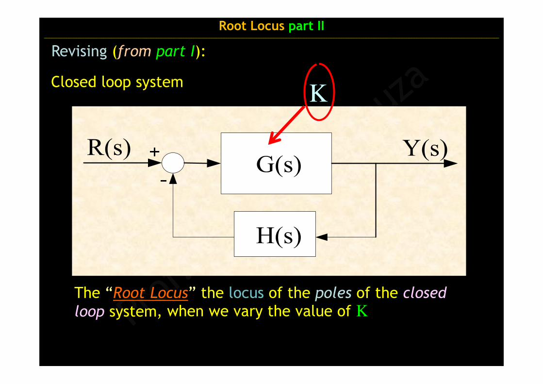
Closed loop system
The “Root Locus” the locus of the poles of the closed
loop system , when we vary the value of K
K
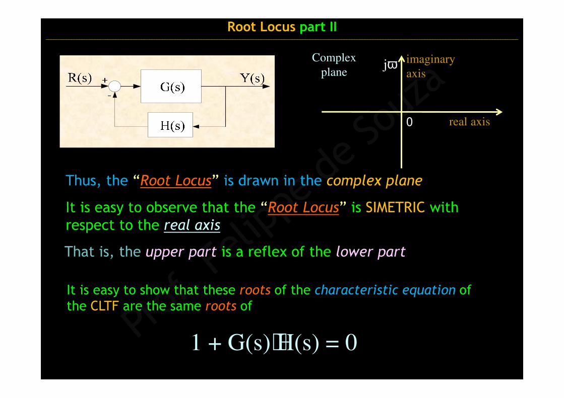
Thus, the “Root Locus” is drawn in the complex plane
That is, the upper part is a reflex of the lower part
Complex
plane
real axis
imaginary
axis
0
jω
Root Locus part II______________________________________________________________________________________________________________________________________________________________________________________
It is easy to observe that the “Root Locus” is SIMETRIC with respect to the real axis
1 + G(s)⋅H(s) = 0
It is easy to show that these roots of the characteristic equation of the CLTF are the same roots of

Note that the “Root Locus” depend only on the produt
G(s)⋅H(s) and not in G(s) or H(s) separately
Root Locus part II ______________________________________________________________________________________________________________________________________________________________________________________
Is called transfer function of the system in open
loop (OLTF).
The expression
G(s)⋅H(s)
G(s)⋅H(s)(OLTF)
Root Locus part II ______________________________________________________________________________________________________________________________________________________________________________________
Rules for the constructing the “Root Locus”
m = the number of open loop zeros
n = the number of open loop poles
We shall call
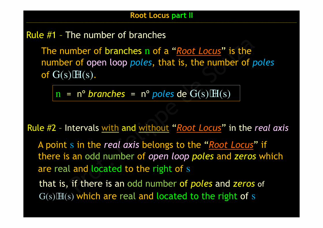
Rule #1 – The number of branches
The number of branches n of a “Root Locus” is the number of open loop poles, that is, the number of poles
of G(s)⋅H(s).
Root Locus part II ______________________________________________________________________________________________________________________________________________________________________________________
n = nº branches = nº poles de G(s)⋅H(s)
Rule #2 – Intervals with and without “Root Locus” in the real axis
that is, if there is an odd number of poles and zeros of
G(s)⋅H(s) which are real and located to the right of s
A point s in the real axis belongs to the “Root Locus” if there is an odd number of open loop poles and zeros which
are real and located to the right of s

Rule #3 – Beginning and end points of the branchesof the “Root Locus”
that is, they start at the n poles of G(s)⋅H(s)
and the remainders:
(n – m) branches of the “Root Locus” finish in the
infinite (∞)
Root Locus part II ______________________________________________________________________________________________________________________________________________________________________________________
The n branches of the “Root Locus” begins in the n de open loop poles
m of the n branches of the “Root Locus” end in the mopen loop zeros
that is, they finish in the m zeros of G(s)⋅H(s)
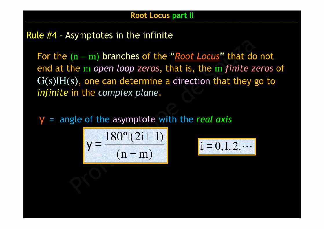
Rule #4 – Asymptotes in the infinite
For the (n – m) branches of the “Root Locus” that do not
end at the m open loop zeros, that is, the m finite zeros of
G(s)⋅H(s), one can determine a direction that they go to infinite in the complex plane.
)mn(
)1i2(º180
−+⋅=γ L,2,1,0i =
γ = angle of the asymptote with the real axis
Root Locus part II ______________________________________________________________________________________________________________________________________________________________________________________

Rule #5 – Point of intersection of the asymptoteswith the real axis
)mn(
)zRe()pRe(n
1i
m
1j
ji
o −
−
=σ
= =
The (n – m) asymptotes in the infinite are well
determined by its directions (angles γ) and by the
point from where they leave the real axis, σo given by the expression:
Root Locus part II ______________________________________________________________________________________________________________________________________________________________________________________
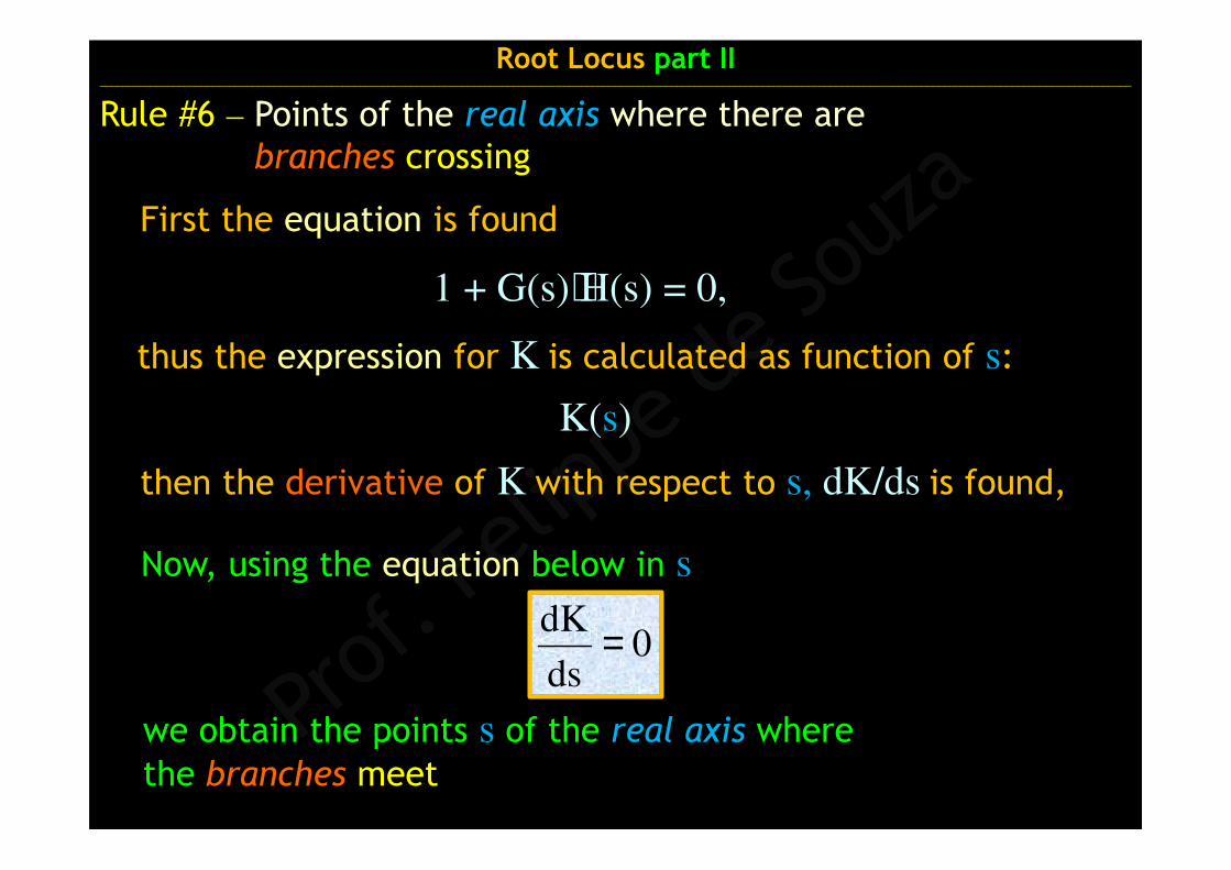
First the equation is found
1 + G(s)⋅H(s) = 0,
Root Locus part II ______________________________________________________________________________________________________________________________________________________________________________________
thus the expression for K is calculated as function of s:
K(s)
then the derivative of K with respect to s, dK/ds is found,
0ds
dK =
we obtain the points s of the real axis where the branches meet
Now, using the equation below in s
Rule #6 – Points of the real axis where there arebranches crossing
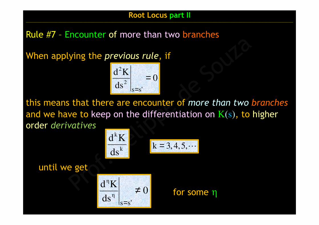
Rule #7 – Encounter of more than two branches
0ds
Kd
s's2
2
==
When applying the previous rule, if
this means that there are encounter of more than two branches
and we have to keep on the differentiation on K(s), to higher order derivatives
k
k
ds
KdL,5,4,3k =
until we get
0ds
Kd
s'sη
η
≠=
for some η
Root Locus part II ______________________________________________________________________________________________________________________________________________________________________________________

this means that there is a meeting of η branches in s’
0ds
Kd
s's
≠=
η
η
If
that is, η branches arrive and η branches leave s’
0ds
Kd
s'sk
k
==
and for ∀ k < η
Root Locus part II ______________________________________________________________________________________________________________________________________________________________________________________
(continued)
In this part II we will see the last rule (Rule #8) and some examples of Root Locus
Rule #7 – Encounter of more than two branches
Rule #8
Crossing points of the “Root Locus” with the imaginary axis
Root Locus part II ______________________________________________________________________________________________________________________________________________________________________________________
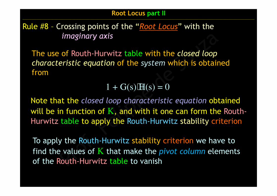
Rule #8 – Crossing points of the “Root Locus” with theimaginary axis
The use of Routh-Hurwitz table with the closed loop
characteristic equation of the system which is obtained from
1 + G(s)⋅H(s) = 0
Note that the closed loop characteristic equation obtained
will be in function of K, and with it one can form the Routh-Hurwitz table to apply the Routh-Hurwitz stability criterion
To apply the Routh-Hurwitz stability criterion we have to
find the values of K that make the pivot column elements of the Routh-Hurwitz table to vanish
Root Locus part II______________________________________________________________________________________________________________________________________________________________________________________
Root Locus part II ______________________________________________________________________________________________________________________________________________________________________________________
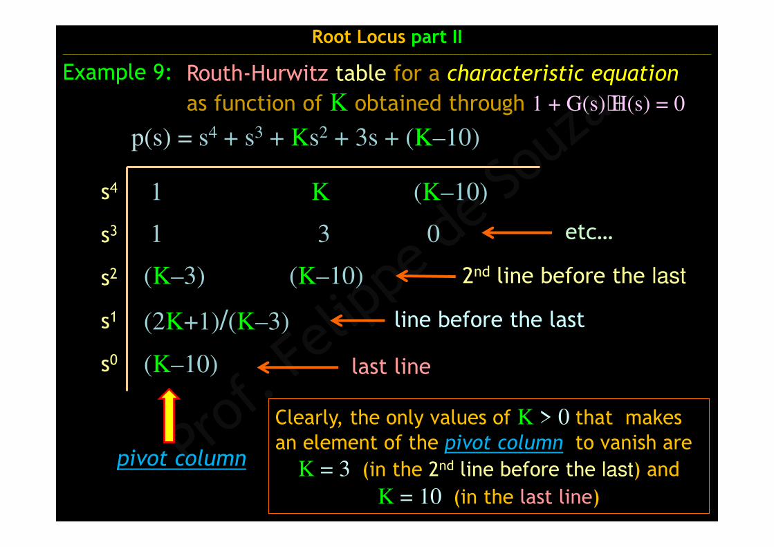
1 K (K–10)
1 3 0
(K–3) (K–10)
(2K+1)/(K–3)
(K–10)
2nd line before the last
s4
s3
s2
s1
s0
Routh-Hurwitz table for a characteristic equation
as function of K obtained through 1 + G(s)⋅H(s) = 0
line before the last
last line
etc…
pivot column
Example 9:
Clearly, the only values of K > 0 that makes an element of the pivot column to vanish are
K = 3 (in the 2nd line before the last) and
K = 10 (in the last line)
p(s) = s4 + s3 + Ks2 + 3s + (K–10)

If ∃ K > 0 that makes elements pivot column to vanish“Root Locus” does not intercept imaginary axis.
If ∃ K > 0 that makes to vanish the LAST element pivot column
“Root Locus” intercepts imaginary axis in
one point, at origin (s = 0).
If ∃ K > 0 that makes to vanish the element before the LAST pivot column
“Root Locus” can intercept imaginary axis in
two points (s = ±jω’).
If ∃ K > 0 that makes to vanish the 2nd element before LAST pivot column
“Root Locus” can intercept imaginary axis in
three points (s = 0 e s = ±jω’).
and so forth …
Root Locus part II______________________________________________________________________________________________________________________________________________________________________________________
Rule #8 – Crossing points of the “Root Locus” with theimaginary axis (continued)

If however, instead of p(s) we calculate the polynomial of
the line immediately above where K makes vanish the pivot column (in Routh-Hurwitz Table), will give us the crossing points of the “Root Locus” with the imaginary axis.
Root Locus part II ______________________________________________________________________________________________________________________________________________________________________________________
In order to know the exact points where the “Root Locus”intercepts the imaginary axis we need to rewrite the
characteristic equation p(s) substituting K for each of the
values of K that makes the elements of pivot column to vanish
In it we will find the eventual crossing points of the “Root
Locus” with the imaginary axis.
After that, we calculate the roots of p(s)
Rule #8 – Crossing points of the “Root Locus” with theimaginary axis (continued)

Root Locus part II ______________________________________________________________________________________________________________________________________________________________________________________
Example 10 Application of Rule #8 –
Crossing points of the “Root Locus” with the imaginary axis
Returning to Example 1 (part I), the characteristic equation of the CLTFis given by:
1 K
K
(2K – 4) (2K – 4) = 0
K = 0
K = 2
Setting up the Routh-Hurwitz table (as function of K):
Analysing where there are K ≥ 0 that makes the elements of pivot
column to vanish, we have that “Root Locus” intercepts the imaginary
axis in 3 points:
s2 + (2K–4) s + K = 0
s2
s1
s0
at the origin for K= 0 and also in ±jω’ when K = 2
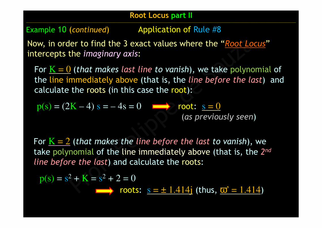
Now, in order to find the 3 exact values where the “Root Locus”intercepts the imaginary axis:
p(s) = (2K – 4) s = – 4s = 0 root: s = 0(as previously seen)
p(s) = s2 + K = s2 + 2 = 0
roots: s = ± 1.414j (thus, ω’ = 1.414)
Root Locus part II ______________________________________________________________________________________________________________________________________________________________________________________
Example 10 (continued) Application of Rule #8
For K = 0 (that makes last line to vanish), we take polynomial of the line immediately above (that is, the line before the last) and calculate the roots (in this case the root):
For K = 2 (that makes the line before the last to vanish), we take polynomial of the line immediately above (that is, the 2nd
line before the last) and calculate the roots:
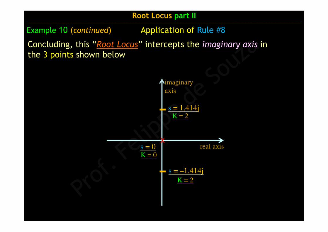
Concluding, this “Root Locus” intercepts the imaginary axis in the 3 points shown below
Root Locus part II______________________________________________________________________________________________________________________________________________________________________________________
Example 10 (continued) Application of Rule #8
s = 1.414j
s = –1.414j
s = 0x
real axis
imaginary
axis
K = 2
K = 2
K = 0
)1s()2s2s(
)2s(K)s(H)s(G
2
2
+⋅++−⋅=
Root Locus part II______________________________________________________________________________________________________________________________________________________________________________________
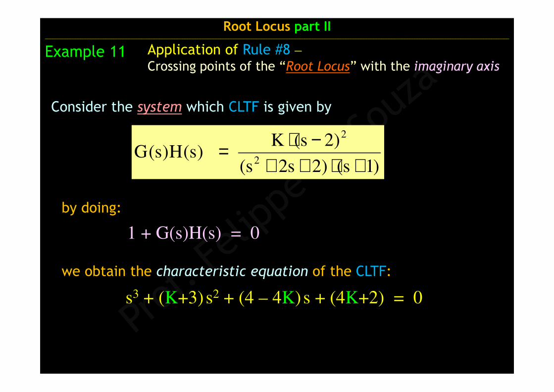
Example 11 Application of Rule #8 –Crossing points of the “Root Locus” with the imaginary axis
we obtain the characteristic equation of the CLTF:
Consider the system which CLTF is given by
s3 + (K+3)s2 + (4 – 4K)s + (4K+2) = 0
by doing:
1 + G(s)H(s) = 0
Root Locus part II______________________________________________________________________________________________________________________________________________________________________________________
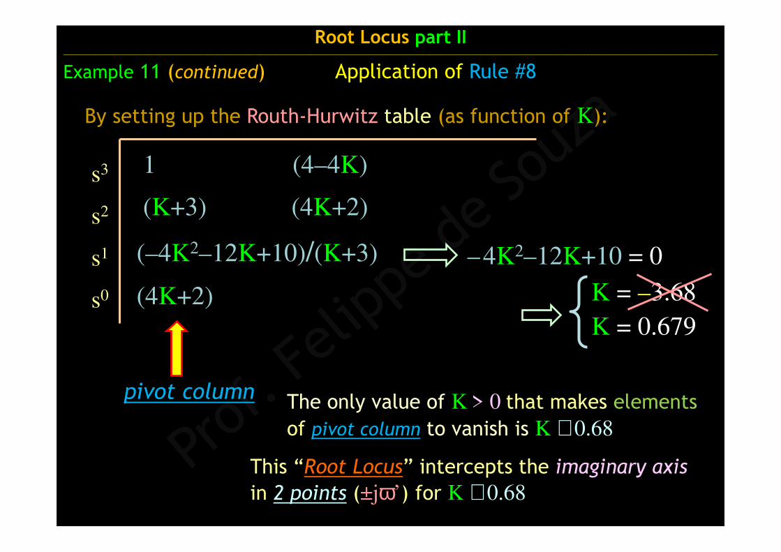
1 (4–4K)
(K+3) (4K+2)
(–4K2–12K+10)/(K+3)
(4K+2)
s3
s2
s1
s0
pivot column
Example 11 (continued) Application of Rule #8
By setting up the Routh-Hurwitz table (as function of K):
–4K2–12K+10 = 0
K = –3.68
K = 0.679
This “Root Locus” intercepts the imaginary axis
in 2 points (±jω’) for K ≅ 0.68
The only value of K > 0 that makes elements
of pivot column to vanish is K ≅ 0.68

Now, in order to find these 2 values (±jω’) where the “Root Locus”
intercept the imaginary axis when K ≅ 0.68, we take the polynomial of the line immediately above (that is, the line before the last) and calculates the roots:
roots: s = ± 1.132j
(thus, ω’ = 1.132)
Root Locus part II______________________________________________________________________________________________________________________________________________________________________________________
Example 11 (continued) Application of Rule #8
s = 1.132j
s = –1.132j
real axis
imaginary
axis
K = 0.68
K = 0.68
Concluding, this “Root Locus”intercepts the imaginary axis in 2 points shown here in the graph
p(s) = (K+3) s2 + (4K+2) = 0
3.68 s2 + 4.72 = 0
Examples
Sketch of the Root Locus (Application of all the rules)
Root Locus part II ______________________________________________________________________________________________________________________________________________________________________________________
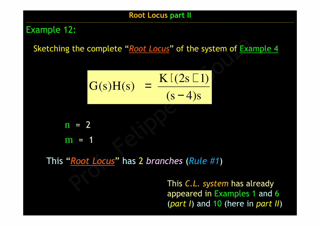
Sketching the complete “Root Locus” of the system of Example 4
s)4s(
)1s2(K)s(H)s(G
−+⋅=
Root Locus part II______________________________________________________________________________________________________________________________________________________________________________________
Example 12:
m = 1
n = 2
This “Root Locus” has 2 branches (Rule #1)
This C.L. system has already appeared in Examples 1 and 6(part I) and 10 (here in part II)
xxo0 4– 0.5
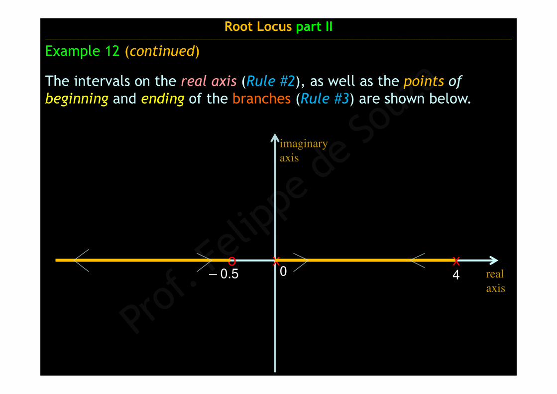
The intervals on the real axis (Rule #2), as well as the points of
beginning and ending of the branches (Rule #3) are shown below.
Root Locus part II______________________________________________________________________________________________________________________________________________________________________________________
Example 12 (continued)
real
axis
imaginary
axis

xo0– 0.5
K = 0K → ∞
Root Locus part II______________________________________________________________________________________________________________________________________________________________________________________
Example 12 (continued)
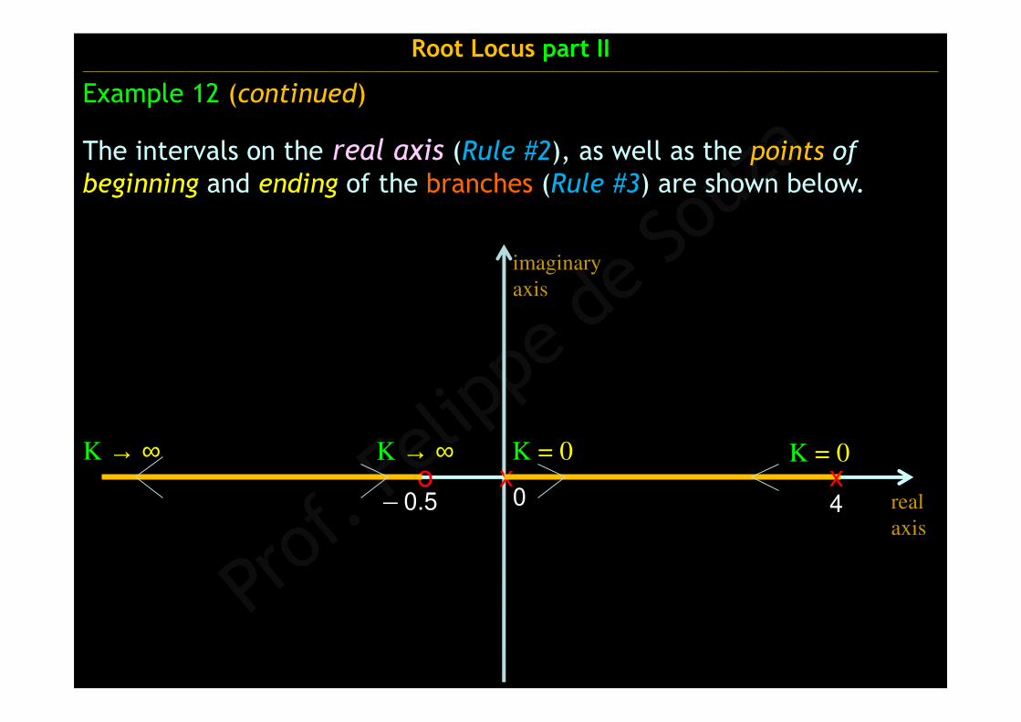
The intervals on the real axis (Rule #2), as well as the points of
beginning and ending of the branches (Rule #3) are shown below.
imaginary
axis
x4 real
axis
imaginary
axis
xo0– 0.5
K → ∞ K → ∞ K = 0 K = 0
Root Locus part II______________________________________________________________________________________________________________________________________________________________________________________
Example 12 (continued)
The intervals on the real axis (Rule #2), as well as the points of
beginning and ending of the branches (Rule #3) are shown below.
x4 real
axis

imaginary
axis
xo0– 0.5
The only asymptote at the infinite occurs in γ = 180º (Rule #4). The meeting point of the asymptote σo = 4.5 (Rule #5), although in this case it is not necessary since the Root Locus lies entirely in the real axis.
K → ∞ K → ∞ K = 0
Root Locus part II______________________________________________________________________________________________________________________________________________________________________________________
Example 12 (continued)
x4
K = 0
real
axis

xo0– 0.5
It is already possible to predict that 2 branches meet on the right and LEAVE the real axis to meet again on the left when they ENTER the real axis again.
K → ∞ K → ∞ K = 0
Root Locus part II______________________________________________________________________________________________________________________________________________________________________________________
Example 12 (continued)
imaginary
axis
K = 0
real
axis
x4

xo0– 0.5
However, only by Rule #6 it will be possible to exactly determine what these points are
K → ∞ K → ∞ K = 0
Rule #6Rule #6
Root Locus part II______________________________________________________________________________________________________________________________________________________________________________________
Example 12 (continued)
imaginary
axis
x4
K = 0
real
axis
xo0– 0.5
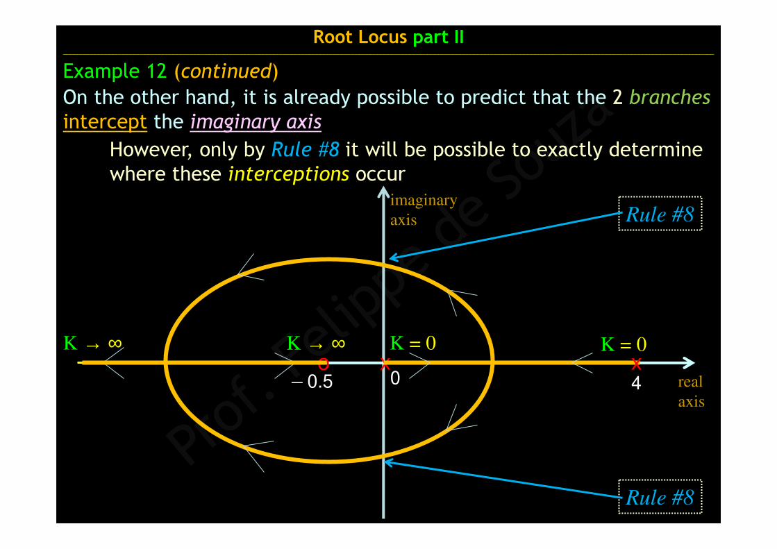
However, only by Rule #8 it will be possible to exactly determine where these interceptions occur
K → ∞ K → ∞ K = 0
Rule #8
Rule #8
Root Locus part II______________________________________________________________________________________________________________________________________________________________________________________
Example 12 (continued)
On the other hand, it is already possible to predict that the 2 branches
intercept the imaginary axis
imaginary
axis
x4
K = 0
real
axis
xo0– 0.5
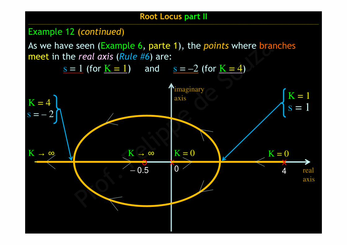
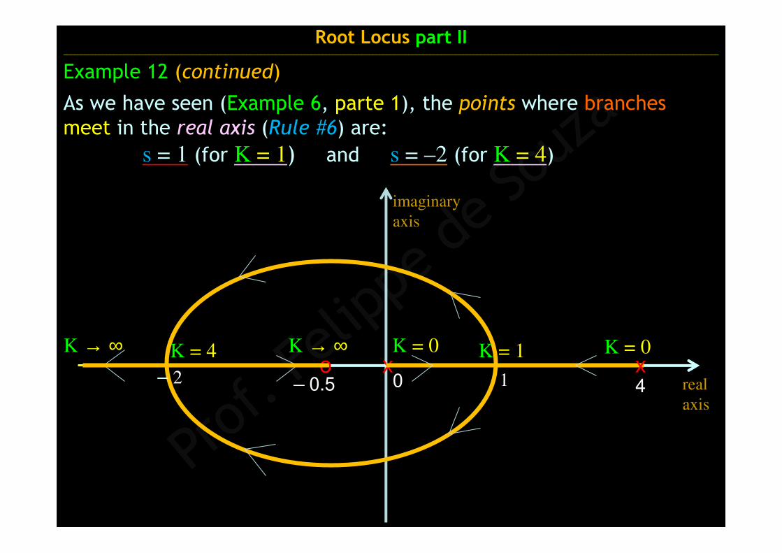
As we have seen (Example 6, parte 1), the points where branches meet in the real axis (Rule #6) are:
s = 1 (for K = 1) and s = –2 (for K = 4)
K → ∞ K → ∞ K = 0
K = 1
s = 1K = 4
s = – 2
Root Locus part II______________________________________________________________________________________________________________________________________________________________________________________
Example 12 (continued)
imaginary
axis
x4
K = 0
real
axis
xo0– 0.5
K → ∞ K → ∞ K = 0K = 4 K = 1
– 2
Root Locus part II______________________________________________________________________________________________________________________________________________________________________________________
Example 12 (continued)
As we have seen (Example 6, parte 1), the points where branches meet in the real axis (Rule #6) are:
s = 1 (for K = 1) and s = –2 (for K = 4)
imaginary
axis
x41
K = 0
real
axis

xo0– 0.5
As we have seen (Example 10), the meeting points with imaginary
axis (Rule #8) are:
s = ± 1.414j (for K = 2)
K → ∞ K → ∞ K = 0K = 4 K = 1
– 2
s = 1.414j
K = 2
s = – 1.414j
K = 2
Root Locus part II______________________________________________________________________________________________________________________________________________________________________________________
Example 12 (continued)
imaginary
axis
x41
K = 0
real
axis

xo0– 0.5
K → ∞ K → ∞ K = 0K = 4 K = 1
– 2
1.414j
– 1.414j
K = 2
K = 2
Root Locus part II______________________________________________________________________________________________________________________________________________________________________________________
Example 12 (continued)
imaginary
axis
As we have seen (Example 10), the meeting points with imaginary
axis (Rule #8) are:
s = ± 1.414j (for K = 2)
x41
K = 0
real
axis

xo0– 0.5
and the “Root Locus” now is complete.
K → ∞ K → ∞ K = 0K = 4 K = 1
1– 2
1.414j
– 1.414j
K = 2
K = 2
Root Locus part II______________________________________________________________________________________________________________________________________________________________________________________
Example 12 (continued)
Observe that the C.L. system is
stable if K > 2Since in this case both 2 C.L. poles
lie in the LHP
imaginary
axis
x4
K = 0
real
axis
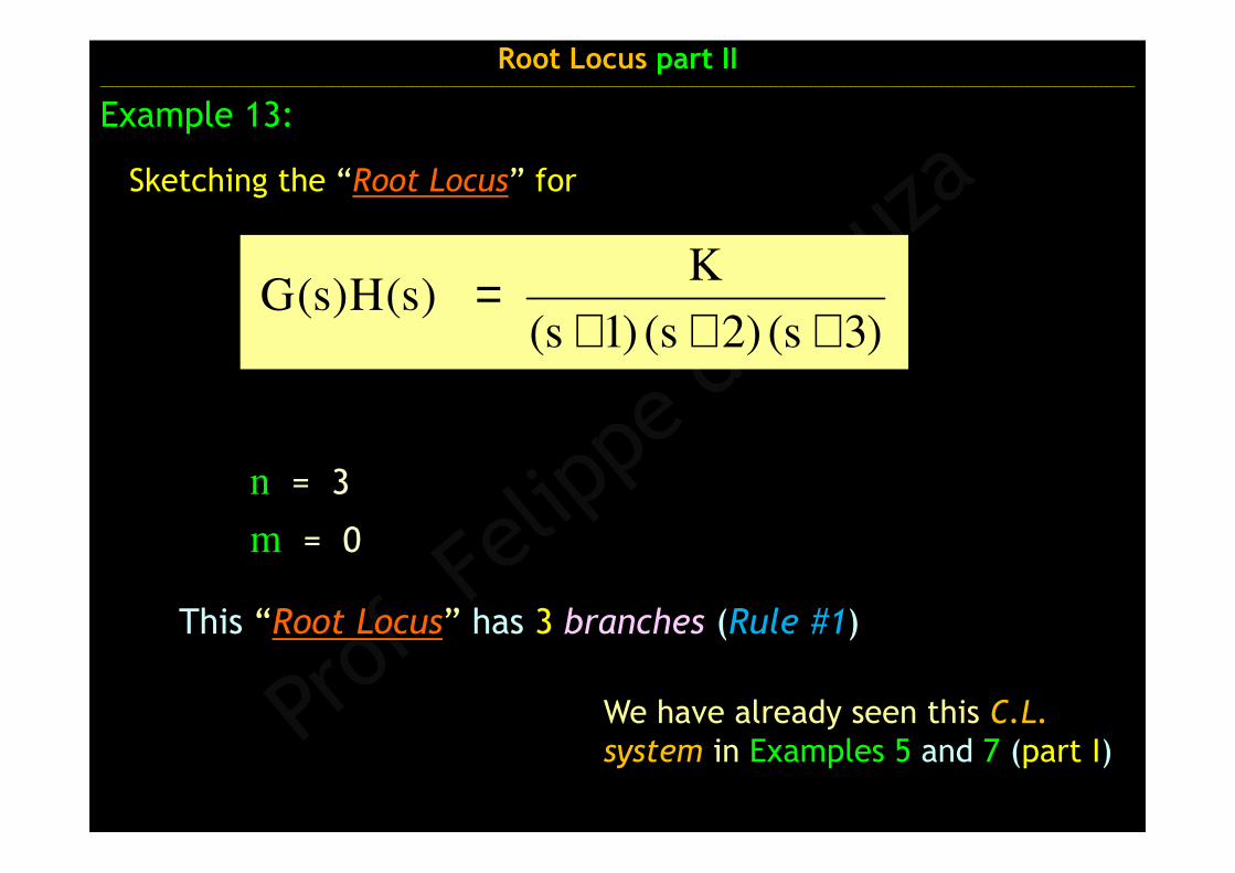
Sketching the “Root Locus” for
)3s()2s()1s(
K)s(H)s(G
+++=
Root Locus part II______________________________________________________________________________________________________________________________________________________________________________________
Example 13:
m = 0
n = 3
This “Root Locus” has 3 branches (Rule #1)
We have already seen this C.L.
system in Examples 5 and 7 (part I)
x– 2
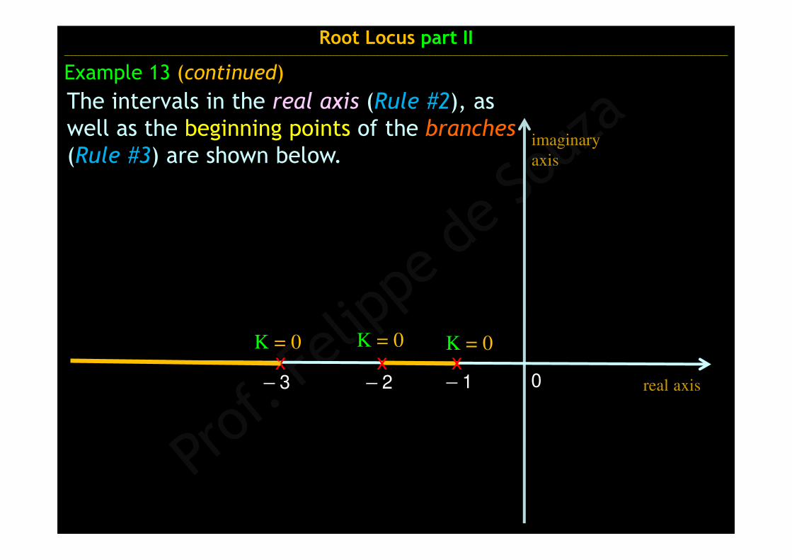
The intervals in the real axis (Rule #2), as well as the beginning points of the branches
(Rule #3) are shown below.
Example 13 (continued)
xx
Root Locus part II ______________________________________________________________________________________________________________________________________________________________________________________
– 3 – 1
K = 0 K = 0K = 0
0 real axis
imaginary
axis

Root Locus part II ______________________________________________________________________________________________________________________________________________________________________________________
Example 13 (continued)
the 3 ending points of the branches (Rule #3)
all lie at the infinite since (n – m) = 3
the crossing point of the asymptote
is σo = –2 (Rule #5)
x– 2
xx– 3 – 1
K = 0 K = 0K = 0
0
as asymptotes at the infinite lie
in γ = ±60º and 180º (Rule #4)
K → ∞
K → ∞
K → ∞
real axis
imaginary
axis
Root Locus part II ______________________________________________________________________________________________________________________________________________________________________________________
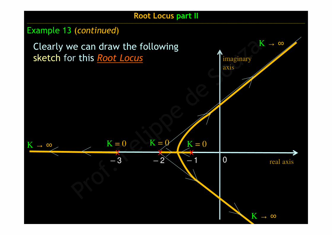
Example 13 (continued)
x– 2
xx– 3 – 1
K = 0 K = 0K = 0
0
K → ∞
K → ∞
K → ∞Clearly we can draw the following sketch for this Root Locus
real axis
imaginary
axis

Root Locus part II ______________________________________________________________________________________________________________________________________________________________________________________
Example 13 (continued)
x– 2
xx– 3 – 1
K = 0 K = 0K = 0
0
K → ∞
K → ∞
K → ∞Clearly we can draw the following sketch for this Root Locus
Rule #8
Rule #6
Rule #8
real axis
imaginary
axis
Root Locus part II ______________________________________________________________________________________________________________________________________________________________________________________
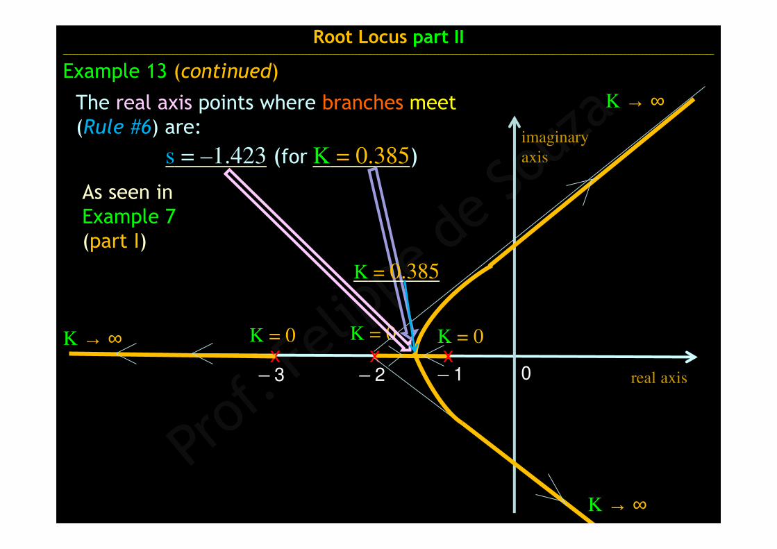
Example 13 (continued)
The real axis points where branches meet(Rule #6) are:
s = –1.423 (for K = 0.385)
x– 2
xx– 3 – 1
K = 0 K = 0K = 0
0
K → ∞
K → ∞
K → ∞
K = 0.385
As seen in Example 7(part I)
real axis
imaginary
axis
Root Locus part II ______________________________________________________________________________________________________________________________________________________________________________________
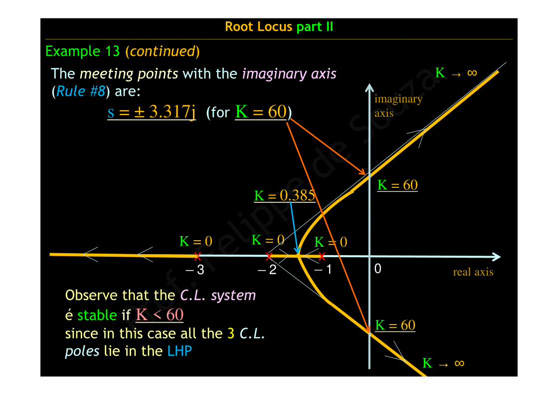
Example 13 (continued)
The meeting points with the imaginary axis
(Rule #8) are:
s = ± 3.317j (for K = 60)
x– 2
xx– 3 – 1
K = 0 K = 0K = 0
0
K → ∞
K → ∞
K = 60
K = 60
Observe that the C.L. system
é stable if K < 60since in this case all the 3 C.L.
poles lie in the LHP
K = 0.385
real axis
imaginary
axis

Example 14:
)1s()2s2s(
)2s(K)s(H)s(G
2
2
+⋅++−⋅=
Root Locus part II______________________________________________________________________________________________________________________________________________________________________________________
Sketching the “Root Locus” for
This “Root Locus” has 3 branches (Rule #1)
m = 2
n = 3
We have already seen this C.L. system
in Example 11 (here in part II)
o
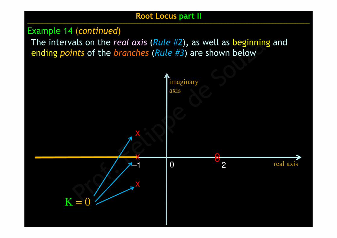
The intervals on the real axis (Rule #2), as well as beginning and ending points of the branches (Rule #3) are shown below
Example 14 (continued)
x o
Root Locus part II______________________________________________________________________________________________________________________________________________________________________________________
real axis
imaginary
axis
x
x
2–1 0
K = 0
K → ∞K → ∞
ox o
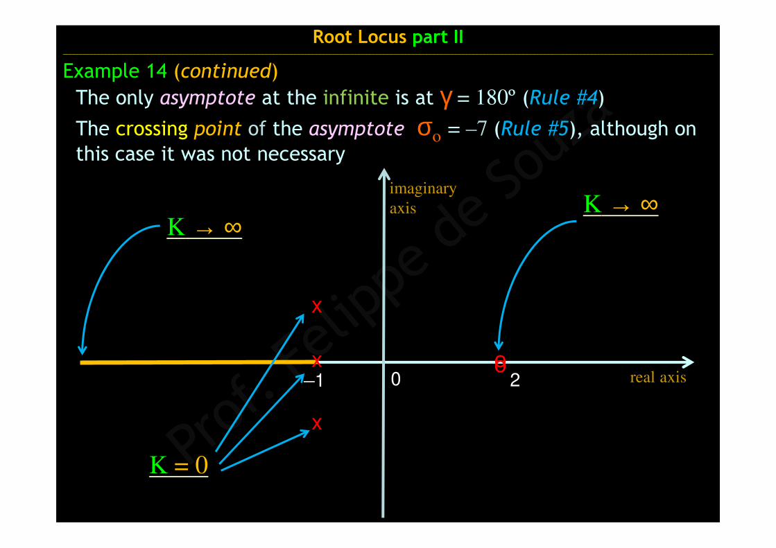
The only asymptote at the infinite is at γ = 180º (Rule #4)
The crossing point of the asymptote σo = –7 (Rule #5), although on this case it was not necessary
Root Locus part II______________________________________________________________________________________________________________________________________________________________________________________
Example 14 (continued)
real axis
imaginary
axis
x
x
2–1 0
K = 0
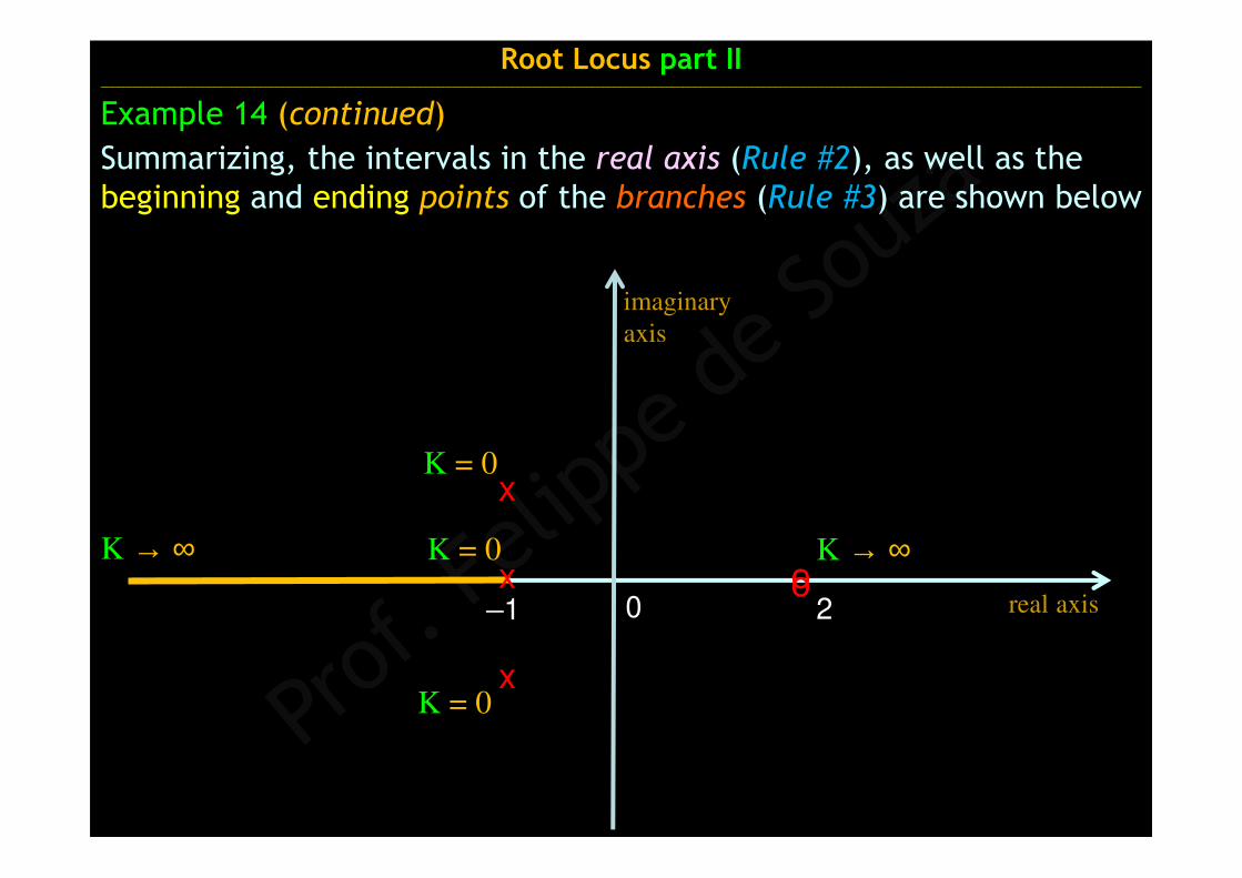
Summarizing, the intervals in the real axis (Rule #2), as well as the beginning and ending points of the branches (Rule #3) are shown below
K → ∞ox o
K = 0
Root Locus part II ______________________________________________________________________________________________________________________________________________________________________________________
Example 14 (continued)
real axis
imaginary
axis
x
xK = 0
K = 0
2–1 0
K → ∞

K → ∞ox o
K → ∞K = 0
We ca predict that 2 branches that start at the 2 complex poles
s = –1 ± j go to the right to meet the double zeros at s = 2
Root Locus part II ______________________________________________________________________________________________________________________________________________________________________________________
Example 14 (continued)
real axis
imaginary
axis
x
xK = 0
K = 0
2–1 0

oo
besides, a third branch, that start at the real pole at s = – 1 goes
to the left to lie on the asymptote at the ∞
Root Locus part II ______________________________________________________________________________________________________________________________________________________________________________________
Example 14 (continued)
real axis
imaginary
axis
2–1 0x
x
x
K → ∞ K → ∞K = 0
K = 0
K = 0
oo
Root Locus part II ______________________________________________________________________________________________________________________________________________________________________________________
Example 14 (continued)
real axis
imaginary
axis
2–1 0x
x
x
K → ∞ K → ∞K = 0
K = 0
K = 0
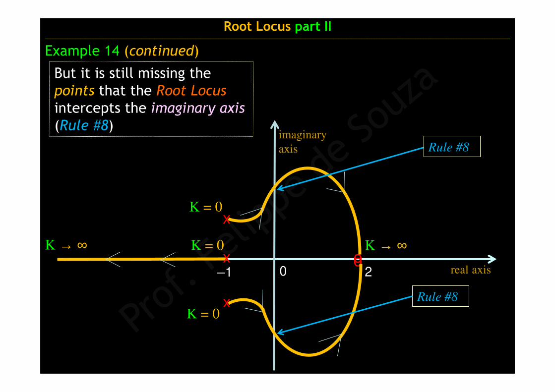
But it is still missing the points that the Root Locus
intercepts the imaginary axis
(Rule #8)
Rule #8
Rule #8
oo
Example 14 (continued)
real axis
imaginary
axis
2–1 0x
x
x
K → ∞ K → ∞K = 0
K = 0
K = 0
K = 0.679
K = 0.679
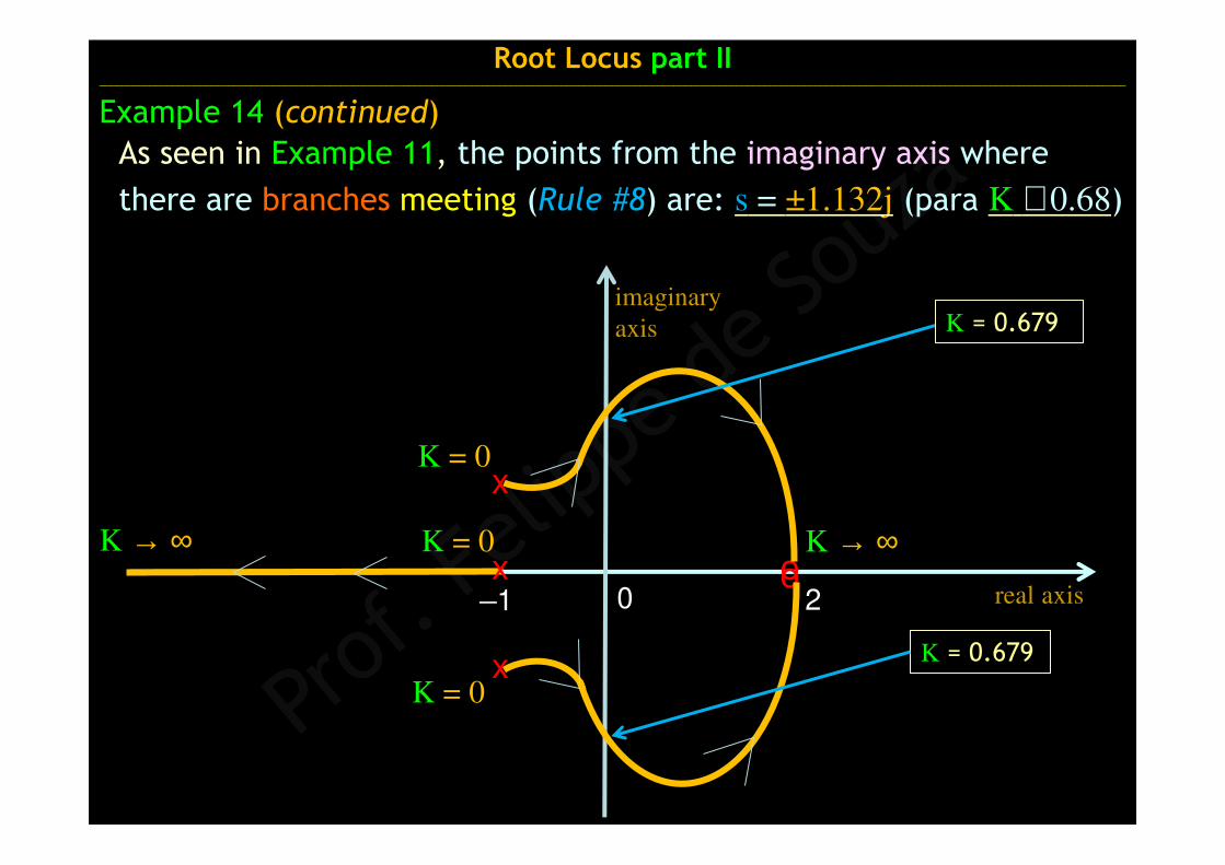
As seen in Example 11, the points from the imaginary axis where
there are branches meeting (Rule #8) are: s = ±1.132j (para K ≅ 0.68)
Root Locus part II ______________________________________________________________________________________________________________________________________________________________________________________
oo
Root Locus part II ______________________________________________________________________________________________________________________________________________________________________________________
Example 14 (continued)
real axis
imaginary
axis
2–1 0x
x
x
K → ∞ K → ∞K = 0
K = 0
K = 0
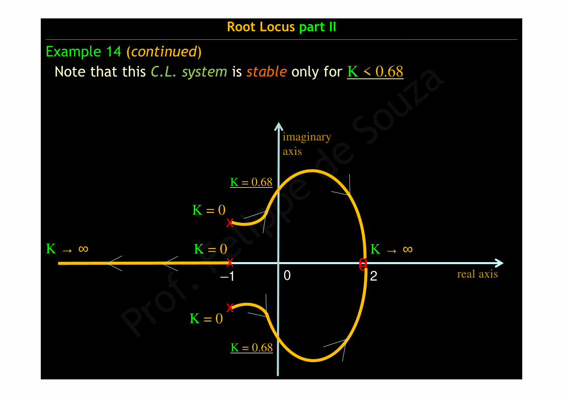
Note that this C.L. system is stable only for K < 0.68
K = 0.68
K = 0.68
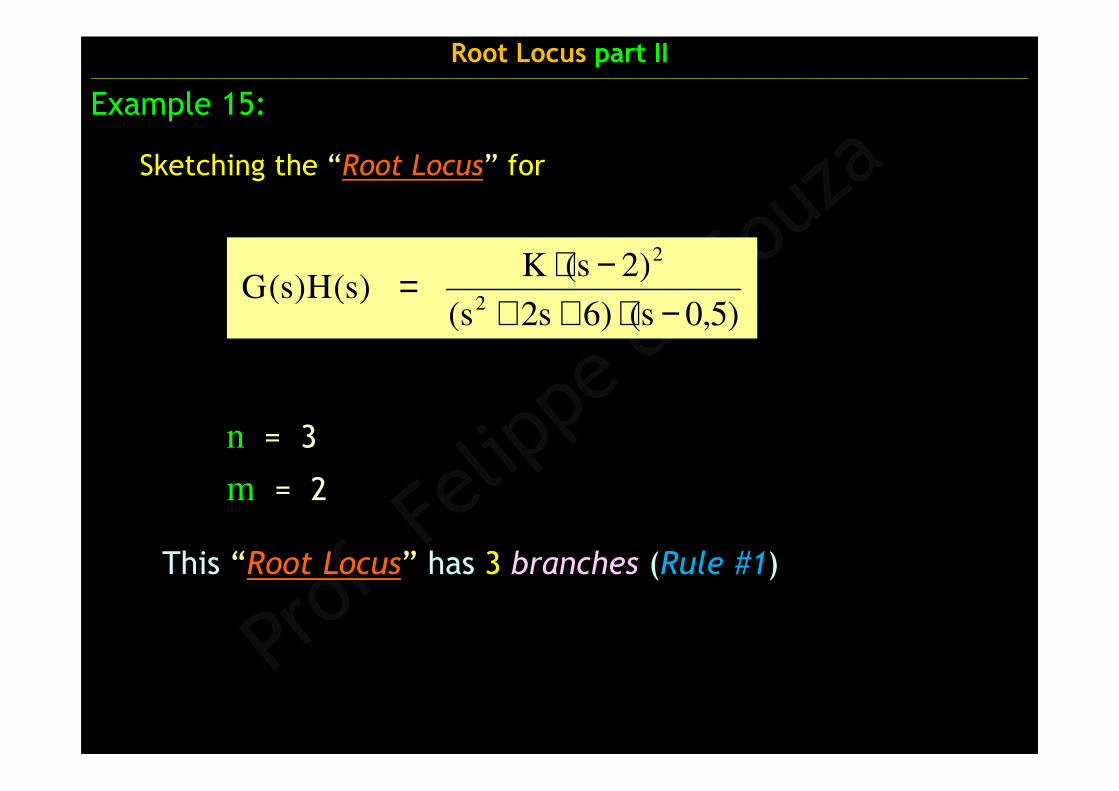
Sketching the “Root Locus” for
)5,0s()6s2s(
)2s(K)s(H)s(G
2
2
−⋅++−⋅=
Root Locus part II ______________________________________________________________________________________________________________________________________________________________________________________
Example 15:
This “Root Locus” has 3 branches (Rule #1)
m = 2
n = 3
x
o20.5
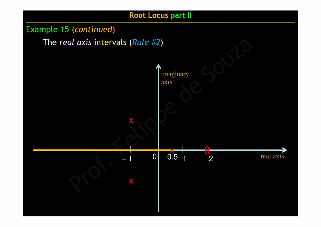
The real axis intervals (Rule #2)
Example 15 (continued)
x o
x
– 1 0
Root Locus part II ______________________________________________________________________________________________________________________________________________________________________________________
real axis
imaginary
axis
1
x
o21
o
x
0
K → ∞
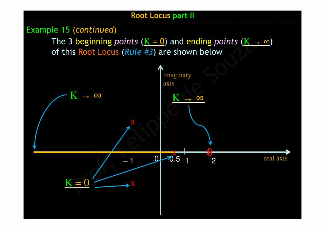
The 3 beginning points (K = 0) and ending points (K → ∞) of this Root Locus (Rule #3) are shown below
K → ∞
K = 0
Root Locus part II______________________________________________________________________________________________________________________________________________________________________________________
Example 15 (continued)
real axis
imaginary
axis
x0.5– 1

x
o21
o
x
0
K → ∞
K = 0
K → ∞K = 0
K = 0
Root Locus part II ______________________________________________________________________________________________________________________________________________________________________________________
Example 15 (continued)
real axis
imaginary
axis
x0.5– 1
The 3 beginning points (K = 0) and ending points (K → ∞) of this Root Locus (Rule #3) are shown below
x
o21
o
x
K → ∞
K = 0
K → ∞K = 0
K = 0
Root Locus part II______________________________________________________________________________________________________________________________________________________________________________________
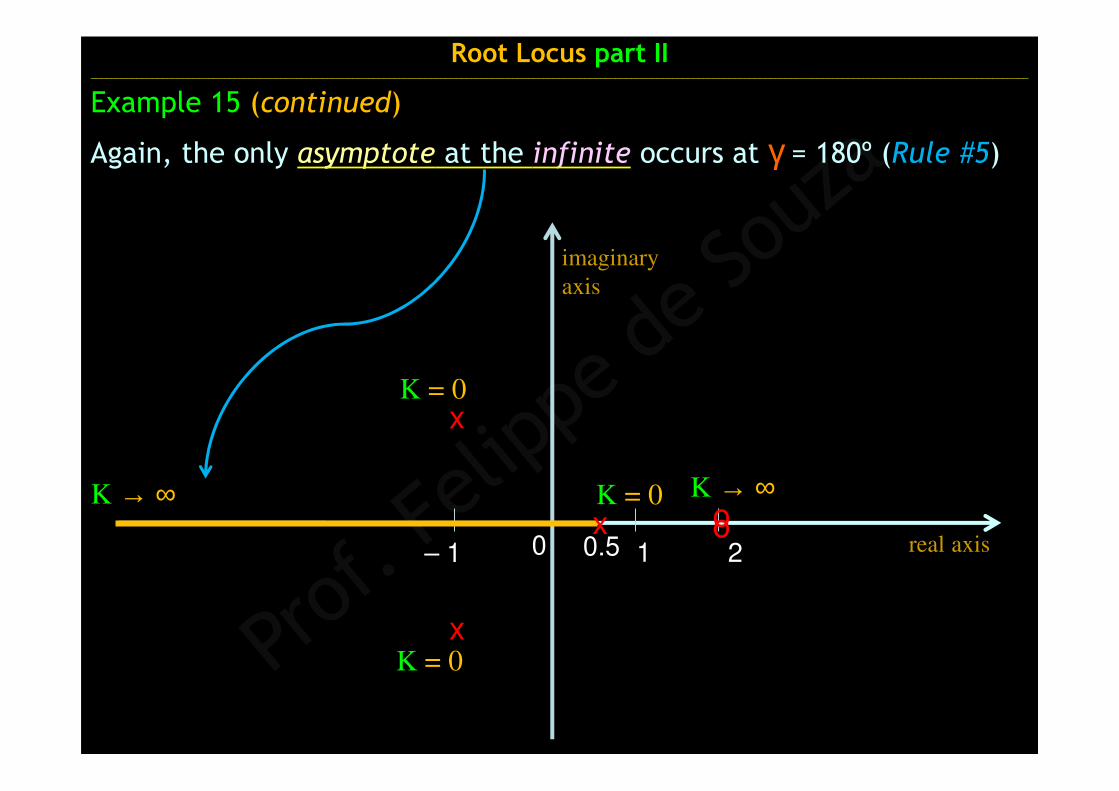
Example 15 (continued)
real axis
imaginary
axis
Again, the only asymptote at the infinite occurs at γ = 180º (Rule #5)
x0 0.5– 1

By Rule #6, this Root Locus has branches meeting at
s = – 1 (for K = 0.833) and s = – 0.531 (for K = 0.84)
x
o21
o
x
K → ∞
K = 0
K → ∞K = 0
K = 0
Root Locus part II ______________________________________________________________________________________________________________________________________________________________________________________
Example 15 (continued)
real axis
imaginary
axis
x0 0.5– 1
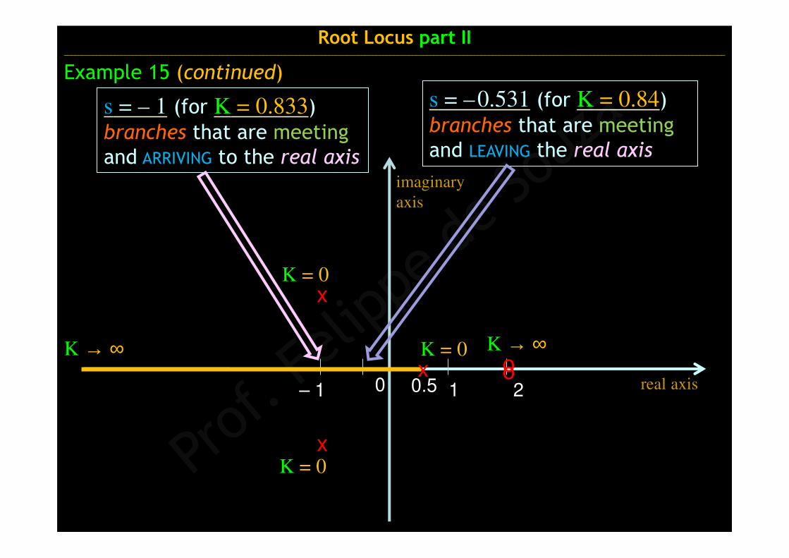
s = – 1 (for K = 0.833) branches that are meetingand ARRIVING to the real axis
x
o21
o
x
K → ∞
K = 0
K → ∞K = 0
K = 0
Root Locus part II ______________________________________________________________________________________________________________________________________________________________________________________
Example 15 (continued)
real axis
imaginary
axis
s = –0.531 (for K = 0.84) branches that are meetingand LEAVING the real axis
x0 0.5– 1
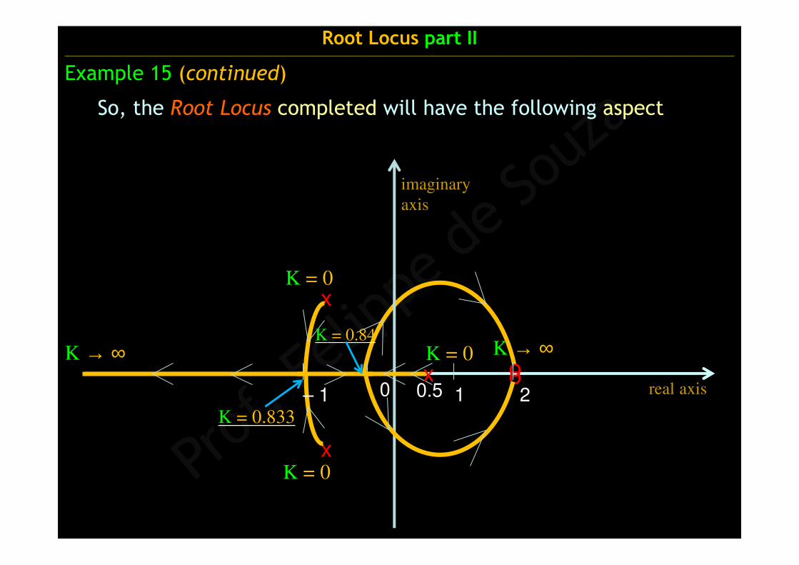
So, the Root Locus completed will have the following aspect
x
o21
o
x
K → ∞xK = 0K → ∞
K = 0
K = 0
K = 0.833
Example 15 (continued)
real axis
imaginary
axis
0 0.5– 1
K = 0.84
Root Locus part II ______________________________________________________________________________________________________________________________________________________________________________________

x
o21
o
x
K → ∞K = 0K → ∞
K = 0
K = 0
Root Locus part II ______________________________________________________________________________________________________________________________________________________________________________________
Example 15 (continued)
real axis
imaginary
axis
x
But it is still missing the points that the Root Locus
intercepts the imaginary axis
(Rule #8)Rule #8
Rule #8
Rule #8
0 0.5– 1
K = 0.84
K = 0.833
K = 0.75
K = 1.1116
x
o21
o
x
K → ∞xK = 0K → ∞
K = 0
K = 0
Root Locus part II ______________________________________________________________________________________________________________________________________________________________________________________
Example 15 (continued)
real axis
imaginary
axis
K = 1.1116
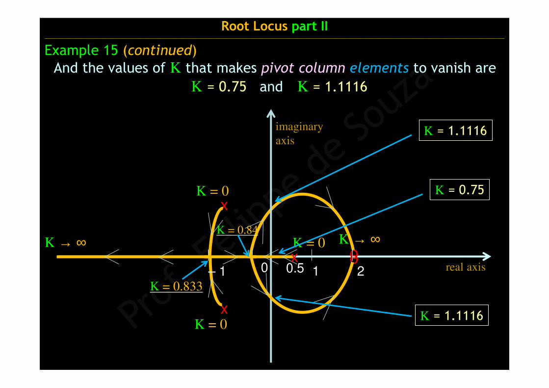
And the values of K that makes pivot column elements to vanish are
K = 0.75 and K = 1.1116
0 0.5– 1
K = 0.84
K = 0.833
x
o2
K=0.75
1
o
x
x
K → ∞K = 0K → ∞
K = 0
K = 0
0.5
Root Locus part II ______________________________________________________________________________________________________________________________________________________________________________________
Example 15 (continued)
real axis
imaginary
axis
K = 1.1116
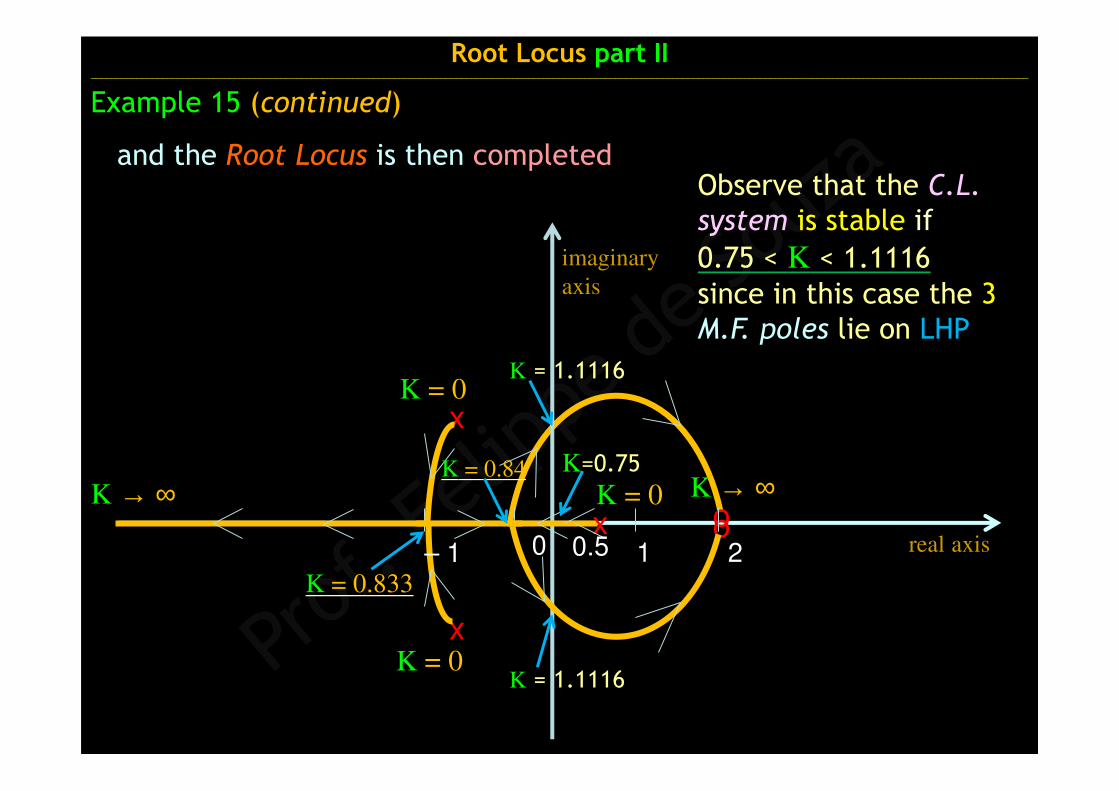
Observe that the C.L.
system is stable if
0.75 < K < 1.1116since in this case the 3 M.F. poles lie on LHP
K = 1.1116
and the Root Locus is then completed
0– 1
K = 0.84
K = 0.833