12 TR ERDC/ Ordinary High Flows and the Stage–Discharge ...

ERD

C/C

RR

EL T

R-1

1-1

2

Wetland Regulatory Assistance Program

Ordinary High Flows and the Stage–Discharge Relationship in the Arid West Region

Katherine E. Curtis, Robert W. Lichvar, and Lindsey E. Dixon July 2011

Co

ld R

egi

on

s R

ese

arc

h

an

d E

ngi

ne

eri

ng

Lab

ora

tory

Approved for public release; distribution is unlimited.

Wetland Regulatory Assistance Program

ERDC/CRREL TR-11-12 July 2011


Katherine E. Curtis, Robert W. Lichvar, and Lindsey E. Dixon

Cold Regions Research and Engineering Laboratory U.S. Army Engineer Research and Development Center 72 Lyme Road Hanover, NH 03755

Approved for public release; distribution is unlimited.

Prepared for U.S. Army Corps of Engineers Washington, DC 20314-1000

ERDC/CRREL TR-11-12 ii

Abstract: The Ordinary High Water Mark (OHWM) defines the lateral extent of non-wetland waters and is regulated as “Waters of the United States” under Sec. 404 of the Clean Water Act. Previous research has developed a reliable and repeatable methodology for identifying the OHWM on ephemeral and intermittent streams in the Arid West using the physical features of the channel (Lichvar and McColley 2008, Curtis and Lichvar 2010). This study expands upon the previous reports by providing an analysis of how gage data may be utilized in OHW determinations. We clarify the methodology for using gage data, review the potential errors encountered in developing a stage–discharge relationship, compare the position of the gage-predicted OHWM to the field OHW signature, and determine the recurrence interval and flow duration of OHW events. The field OHW signature often is not associated with a 2-year flood event like many assume, but ranges from <1- to 15.5-year flood event. This large variation in recurrence intervals for the field OHWMs makes it impossible to define the frequency of the ordinary high flow from gage data because the OHW event is unique to each channel.

DISCLAIMER: The contents of this report are not to be used for advertising, publication, or promotional purposes. Citation of trade names does not constitute an official endorsement or approval of the use of such commercial products. All product names and trademarks cited are the property of their respective owners. The findings of this report are not to be construed as an official Department of the Army position unless so designated by other authorized documents. DESTROY THIS REPORT WHEN NO LONGER NEEDED. DO NOT RETURN IT TO THE ORIGINATOR.

ERDC/CRREL TR-11-12 iii

Table of Contents List of Figures and Tables...................................................................................................................... iv

Preface .....................................................................................................................................................vi

Unit Conversion Factors........................................................................................................................vii

Acronyms.................................................................................................................................................vii

1 Introduction...................................................................................................................................... 11.1 Background .....................................................................................................................11.2 Objective..........................................................................................................................21.3 Approach .........................................................................................................................2

2 Arid West Ephemeral and Intermittent Channel Morphology................................................... 4

3 Gage Data and the Stage–Discharge Relationship.................................................................... 93.1 Developing the stage–discharge relationship ..............................................................93.2 Potential errors of the stage–discharge relationship................................................ 12

4 Site Descriptions ...........................................................................................................................15

5 Methods..........................................................................................................................................21

6 Results ............................................................................................................................................296.1 Instability in the stage–discharge relationship.......................................................... 296.2 Comparison between the field and gage-predicted OHWM recurrence

intervals ........................................................................................................................ 36

7 Discussion ......................................................................................................................................527.1 Finding the OHWM from gage data: perpendicular to the gage versus

upstream from the gage.............................................................................................. 527.2 Instability in the stage–discharge relationship.......................................................... 547.3 Recurrence intervals of the field OHW ....................................................................... 567.4 Limitations of using gage data to define the OHW event ......................................... 59

8 Conclusion......................................................................................................................................63

References.............................................................................................................................................64

Report Documentation Page...............................................................................................................67

ERDC/CRREL TR-11-12 iv

List of Figures and Tables

Figures

Figure 1. Hydrogeomorphic floodplain units of a typical ephemeral or intermittent stream in the Arid West ............................................................................................................................................4Figure 2. Flow indicators and characteristics of the low-flow channel ..................................................5Figure 3. Flow indicators and characteristics of the active floodplain ..................................................6Figure 4. OHWM geomorphic signature .................................................................................................... 6Figure 5. Flow indicators and characteristics of the 100-year floodplain .............................................7Figure 6. Characteristics of the ancient terrace .......................................................................................8Figure 7. USGS gage with a staff outside the gage ...............................................................................10Figure 8. Rating curve showing a stage–discharge relationship .........................................................10Figure 9. Channel cross section divided into verticals ..........................................................................11Figure 10. Locations of USGS gage stations used in this study ..........................................................16Figure 11. Typical flood hydrograph for an ephemeral or intermittent stream in the Arid West .............................................................................................................................................................20Figure 12. Daily instantaneous peak discharge percent greater than the daily mean discharge at Agua Fria ...............................................................................................................................20Figure 13. Flood Frequency Analysis from HEC-SSP of Moenkopi Wash based on Bulletin 17B guidelines ...........................................................................................................................................22Figure 14. Annual peak streamflow for Moenkopi Wash .....................................................................22Figure 15. Shift-adjusted rating curve for Moenkopi Wash ..................................................................23Figure 16. Level and stadia rod used to determine the stage of the field OHWM and the position on the channel bank of the gage-predicted OHWM ...............................................................25Figure 17. Line for measuring the field OHWM perpendicular to the gage for the most accurate stage recording ..........................................................................................................................26Figure 18. Changes in channel morphology and vegetation at Mission Creek .................................30Figure 19. Flood hydrographs for the last decade at Mission Creek ..................................................31Figure 20. Changes in channel morphology and vegetation at Mojave River ....................................32Figure 21. Flood hydrographs for the last decade at Mojave River ....................................................33Figure 22. Changes in channel morphology and vegetation at New River .........................................34Figure 23. Flood hydrographs for the last decade at New River ..........................................................35Figure 24. OHWM at Mission Creek ........................................................................................................37Figure 25. Aerial view of Mission Creek showing the position of GPS points collected ....................37Figure 26. Cristianitos Creek, looking downstream towards the gage at the bridge ........................39Figure 27. Channel characteristics at Santa Maria ...............................................................................40Figure 28. Stage along drift lines and the 100-year floodplain for Santa Maria ...............................40Figure 29. Gage at Mojave River, located beneath the railroad tracks ..............................................41Figure 30. Channel characteristics at Rio Puerco .................................................................................42Figure 31. Annual peak streamflow at Rio Puerco ................................................................................42

ERDC/CRREL TR-11-12 v

Figure 32. Moenkopi Wash ......................................................................................................................43Figure 33. Palm Canyon Wash .................................................................................................................44Figure 34. New River .................................................................................................................................45Figure 35. Agua Fria ..................................................................................................................................46Figure 36. Channel characteristics at Dry Beaver Creek ......................................................................47Figure 37. Channel characteristics at Black Creek ...............................................................................48Figure 38. Deer Creek ...............................................................................................................................49Figure 39. Rock Creek ...............................................................................................................................50Figure 40. Hassayampa River ..................................................................................................................51

Tables

Table 1. 2002 nationwide permit definitions of stream channels .....................................................1Table 2. Characteristics of the study sites ..............................................................................................17Table 3. Ecoregions throughout the Arid West adopted from Bailey (1995) .....................................18Table 4. Flow analysis of the calculated gage-predicted OHWM and the flow dynamics of the field OHWM ..........................................................................................................................................24Table 5. Percentage of days missing since the last gage-predicted ordinary high flow and the cumulative number of hours the field OHWM was exceeded in the past year, past decade, and past two decades ................................................................................................................28

ERDC/CRREL TR-11-12 vi

Preface

This research was funded by the Wetland Regulatory Assistance Program (WRAP), Headquarters, U.S. Army Corps of Engineers (USACE).

This report was prepared by Katherine E. Curtis, Robert W. Lichvar, and Lindsey E. Dixon, all of the Remote Sensing/Geographic Information Systems (RS/GIS) and Water Resources Branch, Cold Regions Research and Engineering Laboratory (CRREL), U.S. Army Engineer Research and Development Center (ERDC), Hanover, NH. This study was conducted under the general supervision of Timothy Pangburn, Chief, RS/GIS and Water Resources Branch; Dr. Justin B. Berman, Chief, Research and Engineering Division; Dr. Lance Hansen, Deputy Director; and Dr. Robert E. Davis, Director. Permission to publish was granted by Director, Cold Regions Research and Engineering Laboratory.

The authors thank Meredith L. Carr and Erin E. Black for providing technical reviews of this document.

COL Kevin J. Wilson was the Commander and Executive Director of ERDC, and Dr. Jeffery P. Holland was the Director.

ERDC/CRREL TR-11-12 vii

Unit Conversion Factors

Multiply By To Obtain

cubic feet per second (cfs) 0.02831685 cubic meters per second

feet 0.3048 meters

yards 0.9144 meters

miles (U.S. statute) 1,609.347 meters

Acronyms

ADCP Acoustic Doppler current profiler

CFR Code of Federal Regulations

cfs Cubic feet per second

FFA Flood Frequency Analysis

gps Global positioning system

GZF Gage height of zero flow

HEC-SSP Hydrologic Engineering Center Statistical Software Package

OHW Ordinary High Water

OHWM Ordinary High Water Mark

USACE United States Army Corps of Engineers

USGS United States Geological Survey

WoUS Waters of the United States

ERDC/CRREL TR-11-12 1

1 Introduction

1.1 Background

The Ordinary High Water Mark (OHWM) defines the lateral extent of non-wetland waters in ephemeral and intermittent streams in the Arid West. These channels are regulated as “Waters of the United States” (WoUS) under Sec. 404 of the Clean Water Act. The OHWM is the boundary between two distinct hydrogeomorphic floodplain surfaces: the active floodplain and the 100-year floodplain. This boundary is defined by a “line on the shore established by fluctuations of water and indicated by physical characteristics such as a clear, natural line impressed on the bank, shelving, changes in character of the soil, destruction of terrestrial vegetation, or the presence of litter and debris” (33 CFR Part 328.3). In Arid West ephemeral and intermittent streams, the flashiness of storm events and the frequent shifting of the channel morphology often make it challenging to identify the OHWM. “A Field Guide to the Identification of the Ordinary High Water Mark (OHWM) in the Arid West Region of the Western United States” (Lichvar and McColley 2008) was developed to address these uncertainties and to provide consistency in delineating the OHWM.

Ephemeral and intermittent channels differ from perennial channels in that they have significant periods of time without flow (Table 1). In Arid West ephemeral and intermittent streams, the channel-forming discharge

Table 1. 2002 nationwide permit definitions of stream channels (USACE 2002).

Channel type Definition

Ephemeral An ephemeral stream has flowing water only during, and for a short duration after, precipitation events in a typical year. Ephemeral stream beds are located above the water table year-round. Groundwater is not a source of water for the stream. Runoff from rainfall is the primary source of water for stream flow.

Intermittent An intermittent stream has flowing water during certain times of the year, when groundwater provides water for stream flow. During dry periods, intermittent streams may not have flowing water. Runoff from rainfall is a supplemental source of water for stream flow.

Perennial A perennial stream has flowing water year-round during a typical year. The water table is located above the stream bed for most of the year. Groundwater is the primary source of water for stream flow. Runoff from rainfall is a supplemental source of water for stream flow.


is defined by the ordinary high flow. This ordinary high discharge is a low to moderate flood event (Lichvar et al. 2006) that is responsible for establishing and maintaining the outer boundary of the active floodplain (Riggs 1985). The majority of sediment transport in a stream occurs within this active channel.

1.2 Objective

The OHWM, the most reliable and repeatable boundary in the channel, is best identified through physical features that create a characteristic geomorphic signature (Lichvar and McColley 2008). The Arid West manual and a supplemental revised datasheet (Curtis and Lichvar 2010) provide clear and concise methodology for how to identify the geomorphic signature in the field to find the lateral extent of the OHWM. Additionally, they describe how to use supplemental data such as aerial photographs and geologic maps to delineate the OHWM. However, only a preliminary explanation of how to use gage data is provided. This study expands on the manuals and explores the feasibility of using gage data in OHWM delineation more extensively. This report includes (1) background on Arid West OHW; (2) a brief description of how the stage–discharge relationship is developed and an overview of the errors associated with the process; (3) a revised methodology that explains the procedure for using gage data to identify the OHWM; (4) site examples that demonstrate the challenges and limitations associated with using gage data to identify the OHWM; (5) a systematic comparison of the differences between the gage-predicted OHWM and the field OHWM; and (6) an analysis of the field OHWM recurrence intervals.

1.3 Approach

To understand the feasibility of using gage data to improve the OHW delineation methodology and increase understanding of the frequency of OHW flows for regulation purposes, we analyzed 14 gaged ephemeral and intermittent streams throughout the Arid West. For each channel, we determined the gage-predicted OHWM, its position on the landscape, and its relationship to the field OHW signature. We used photographs and flow data from the past decade to highlight how low to moderate flows influence the stage–discharge relationship through changes in the channel morphology, sediment texture, and vegetation characteristics in a channel. We determined the field OHWM and, for each site, compared its position to the gage-predicted OHWM and explored what variables may influence


the ordinary high flow recurrence interval. Through this study, we determined the frequency and duration of ordinary high flows throughout the Arid West region and, because of the extreme variation, described the limitations of using gage data to delineate the OHWM.


2 Arid West Ephemeral and Intermittent Channel Morphology

Ephemeral and intermittent streams in the Arid West are frequently characterized by three distinct hydrogeomorphic floodplain units: the low-flow channel, the active floodplain, and the 100-year floodplain (Figure 1). In previous CRREL technical reports, the 100-year floodplain was referred to as the low terrace. However, a terrace is most commonly associated with

Figure 1. Hydrogeomorphic f loodplain units of a typical ephemeral or

intermittent stream in the Arid West.


an abandoned or ancient floodplain. Since this portion of the channel beyond the active floodplain is inundated by extreme events under current conditions, the concept of a 100-year floodplain is more appropriate. Unlike perennial streams, ephemeral and intermittent channels have no bankfull channel because the concept of bankfull is typically associated with a 2-year recurrence interval, which often relates to the frequency of the migratory low-flow channels in these systems (Lichvar et al. 2009). Below, a few of the most common flow indicators and characteristics for each hydrogeomorphic floodplain surface are described.

The low-flow channel has the lowest elevation in the channel and contains water the most frequently. It is characterized by a lack of vegetation (Figure 2A) and often has recent flow indicators such as mudcracks (Figure 2B) or ripples (Figure 2C). The low-flow channel is migratory, frequently filling with sediments and eroding a new part of the channel (Bull 1997). Because it lacks an established position within the channel, it

Figure 2. Flow indicators and characterist ics of the low-f low channel:

(A) lack of vegetation, (B) mudcracks, and (C) r ipples.


is not useful for regulatory purposes. Instead, the outer extent of the active floodplain, the OHWM, is regulated under WoUS in Arid West ephemeral and intermittent streams. The active channel is flooded by low to moderate events (Riggs 1985, Lichvar et al. 2006), and its features depend on the amount of time since the last OHW event. After an ordinary high event, few flow indicators are present in the channel and vegetation is not established (Lichvar et al. 2006). A few years after an event, vegetation on the active floodplain is frequently dominated by young growth (Figure 3A), and the sediment texture is often coarser than in the low-flow channel and the 100-year floodplain (Figure 3B). At the OHWM boundary between the active floodplain and the 100-year floodplain, there is often a defining break in slope (Figure 4A) and a sharp change in vegetation species, percent cover, and successional stage (Figure 4B). Above the active floodplain, the 100-year floodplain is characterized by well-established

Figure 3. Flow indicators and characterist ics of the active f loodplain:

(A) new vegetation growth and (B) change to coarser sediment texture at low-f low boundary.

Figure 4. OHWM geomorphic signature: (A) break in slope and (B) change in vegetation.


vegetation (Figure 5A) and minimal signs of recent flooding. However, flow indicators such as drift (Figure 5B) or fine sediment deposits along tree bark (Figure 5C) may be found on the 100-year floodplain to distinguish it from the ancient terrace. The ancient terrace represents an abandoned floodplain surface and is not flooded under current climatic conditions. It is distinguished from the channel hydrogeomorphic floodplain units by soil development (Figure 6A) and surface rounding (Figure 6B).

Although these flow indicators and characteristics are helpful in classifying the hydrogeomorphic floodplain units, the position of each individual indicator throughout the channel is randomly distributed and the particular event associated with each indicator cannot be determined (Lichvar et al. 2006, Lichvar and McColley 2008). It is therefore necessary to consider the positions of the indicators relative to each other and to the

F igure 5. Flow indicators and characterist ics of the 100-year f loodplain:

(A) establ ished vegetation, (B) drift , and (C) sediment deposits.


Figure 6. Characterist ics of the ancient terrace: (A) soi l development and (B) surface rounding.

hydrogeomorphic floodplain surfaces when delineating the OHWM. For example, mudcracks are remnants of recently ponded water. Although these may occur in low-flow channels, they may also be located in a topographic dip on the 100-year floodplain. The mudcracks therefore do not automatically signify the low-flow channel, but when observed with other physical features of the channel, can be helpful in identifying recent hydrologic conditions. Lichvar and McColley (2008) demonstrated that it is this OHWM geomorphic signature determined from incorporating the relative positions of all indicators in relation to defining channel features such as a break in slope that is the consistent and repeatable characteristic in delineation.

To build on the concepts described in the OHWM manual (Lichvar and McColley 2008), this study explores the potential usefulness of gage data to assist in defining the OHWM. Many people want to apply the perennial bankfull concept of a 1.5- to 2-year event to the OHW signature in ephemeral and intermittent streams and frequently rely on this bankfull concept for numerous water resource projects. However, prior to this study, little was known about the frequency of OHW events in Arid West channels. Understanding if and how gage data may be applied to OHWM delineation is beneficial to regulators, flood management, and under-standing the ecological impacts of these episodic streams.


3 Gage Data and the Stage–Discharge Relationship

U.S. Geological Survey (USGS) gaging stations are critical tools for river management and flood prevention. The data collected at gaging stations is used to describe the flow conditions in streams and to provide an understanding of the magnitude and frequency of past flood events. Gaging stations provide a continuous record of water depth, or stage, which is converted to discharge values through a rating curve. Rating curves are developed individually for each gaging station through numerous field measurements that record the stage and discharge over a wide range of flow magnitudes to develop a stage–discharge relationship. The following section briefly describes the process of developing a stage–discharge relationship and lists common errors associated with this process.

3.1 Developing the stage–discharge relationship

At many USGS gaging stations, the stage is commonly recorded in a still well (Figure 7). The well is connected to the river channel through a pipe that is designed to keep water at the same height in the well as in the channel. A float or an acoustic sensor in the well is used to measure the stage to 0.01-ft accuracy (Olson and Norris 2007). At many gages, these stage measurements are collected every 15 minutes, and data are trans-mitted back to USGS offices to be converted into discharge measurements.

Discharge is a measure of the volume of water that passes through a given area during a period of time. It is impractical to measure discharge continuously; instead, a continuous record of stage data is collected. These data are converted to discharge values using a rating curve that represents the stage–discharge relationship (Figure 8). The rating curve is developed by collecting discharge measurements at a variety of flows and recording the stage when each measurement is collected. A best-fit curve is applied to the graph to represent the stage–discharge relationship.


Figure 7. USGS gage with a staff

outside the gage. The staff shows the height of the water surface used in

developing the stage–discharge relationship.

Figure 8. Rating curve showing a stage–discharge relationship. The

black X’s represent the individual discharge measurements col lected; the blue l ine is a best-f i t curve that is used to convert the stage

measurements col lected in the st i l l wel l to a discharge.


Velocity is measured directly using a current meter, tracer dilution, or acoustic Doppler current profiler (ADCP) or indirectly using methods such as measuring the position of the water line on the bank. To determine the discharge using a current meter (the most common method), a cross section is selected across a stable reach of the channel. The cross section is divided into verticals, and the width, depth, and velocity for each vertical are measured and summed (Figure 9). The equation for calculating discharge using the current meter method is given by Herschy (1994):

(1)

where Q = discharge bi, di, and vi = width, depth, and mean velocity of flow in the ith vertical m = number of verticals.

Figure 9. Channel cross section divided into vert icals, where each individual velocity measurement is col lected using the

current meter method.

These current meter and ADCP discharge measurements are collected on fairly stable reaches or sections of the channel below the gage, called controls. Types of controls include artificial weirs for measuring low flows and naturally occurring physical features such as bedrock banks for higher flows. A more complete description of the types of controls and their significance for developing a stage–discharge relationship may be found in the USGS training course (Nolan et al. 2008) and in Rantz (1982). Controls for the wide, flat, unconsolidated alluvium channels of many ephemeral and intermittent streams in the Arid West are often unstable at all discharges (Kennedy 1984, Tillery et al. 2001), making it challenging to develop reliable stage–discharge relationships. Confined reaches are often ideal positions for gages in perennial streams, but these reaches on ephemeral or intermittent streams are often subject to the most scour and fill (Rantz 1982). Straight reaches are the ideal position for gages on


ephemeral and intermittent streams; however, even these reaches are often unstable and reach equilibrium conditions only briefly (Bull 1997). Consequently, very few Arid West ephemeral and intermittent streams are gaged.

To account for the sediment mobility that alters the stage–discharge relationship, a shift adjustment is applied to the rating curve (Nolan et al. 2008). The gage height of zero flow (GZF), which relates the minimal thalweg position—the lowest elevation in the channel—to a gage height, is checked frequently to ensure there are no changes to the datum (Kennedy 1984). An appropriate adjustment is applied to the rating curve when sediments erode or aggrade.

Ideally eight to ten “out of bank” discharge measurements are required to develop a reliable stage–discharge relationship (USACE 1996). For ephemeral and intermittent streams in the Arid West, “out of bank” refers to flows beyond the active–100-year floodplain boundary. However, channel-forming ordinary high discharges occur very infrequently (Elliott and Cartier 1986) and higher “out of bank” flows are even rarer. When these moderate to large magnitude flows do occur, they are often of such short duration and high intensity that they are not accurately captured in the discharge record. Because the flows are flashy and the high sediment mobility leads to frequent changes to the channel morphology, it is challenging to develop a reliable stage–discharge relationship for ephemeral and intermittent channels in the Arid West. The technical challenges associated with developing a stage–discharge relationship are described more completely below.

3.2 Potential errors of the stage–discharge relationship

Accounting for the high sediment mobility and flashy floods in Arid West ephemeral and intermittent streams is just one of the challenges involved in developing a stage–discharge relationship. Potential errors relating to the stage–discharge relationship can be divided into direct errors and indirect errors. Direct errors, such as changes to the channel morphology and errors associated with current meter measurements, are more easily quantifiable than indirect measurement errors. Indirect measurements are less accurate than direct measurements as they result in errors associated with calculation techniques, such as errors relating stage to discharge when a current meter or ADCP measurement is not available.


Direct errors associated with current meter measurements relate to: (1) the number of verticals used in the measurement; (2) the measurements of depth, width, and velocity for each vertical; (3) the stability of the channel or changes in bedform conditions; (4) rapid changes in stage; (5) changes in flow conditions or unsteady flow effects; (6) changes in water temperature; (7) debris, ice, or wind; and (8) the accuracy of the current meter used to take the measurements. Errors associated with using a current meter can range from 2 to 20% for each individual discharge measurement but are typically between 3 and 6% (Sauer and Meyer 1992). Changes in water temperature influence the viscosity of the water, which in turn affects the channel morphology; a decrease in water temperature may lead to an increase in sand mobility (Rantz 1982). One of the challenges with collecting current meter measurements is that current meters are designed to measure flow directly; the measured velocity may be different from the actual value because of the angle of flow or pulsation errors when the river has an instantaneous higher or lower discharge (Sauer and Meyer 1992).

Ephemeral and intermittent channels are particularly affected by rapidly changing stage, unsteady flow, and channel instability (Bull 1997, Tillery et al. 2001, Nolan et al. 2008, Olson and Norris 2007). The short-duration, high-intensity flows characteristic of the Arid West lead to rapid changes in the water level and flow dynamics. Higher discharges are not accurately measured because of their instantaneous nature, so they must be esti-mated through indirect calculations using high water mark indicators. Similarly, the stage–discharge relationship is often unstable at low flows (Kennedy 1984) because of the frequent migration of low-flow channels in ephemeral and intermittent streams. The highly mobile sediment through-out much of the region frequently aggrades or erodes, making it chal-lenging to develop reliable rating curves. Additionally, the growth and removal of vegetation in the channel bed alters the hydraulic roughness, the channel’s resistance to flow (Bull 1997, Tillery et al. 2001, Nolan et al. 2008). These changes in flow conditions and channel bed morphology affect the reliability of current meter measurements and, subsequently, the accuracy of the stage–discharge relationship.

At best, indirect discharge measurements are within 15% of the actual discharge (Tillery et al. 2001). Indirect errors occur during slope–area, slope–conveyance, and step–backwater computations. Slope–area and slope–conveyance computations involve calculating the discharge post-


flood by identifying high water mark indicators, determining the maxi-mum stage, surveying the channel, and estimating a Manning’s n, the channel hydraulic roughness coefficient. The uncertainties with these indirect measurements relate to the underlying assumption that the conditions present post-flood are the same as those that existed prior to and during the flood event. However, conditions frequently change in sandy ephemeral streams, and the reliability of these methods is question-able. Indirect errors in step–backwater computations can apply to channels where field measurements are not available for high flows. Step–backwater computations involve extrapolating rating curves to the rare discharge events that are not often observed. These computations result in the largest errors, as field conditions are not considered and the estima-tion is purely empirical.

This brief discussion of the potential errors associated with the stage–discharge relationship provides background for understanding the potential errors involved in using gage data to determine the frequency and magnitude of the ordinary high flow. A more complete description of potential errors and the statistical measures used to address these errors may be found in Rantz (1982), Sauer and Meyer (1992), Herschy (1994), USACE (1996), and Clemmens and Wahlin (2006). For information on potential errors specific to ephemeral channels, see Tillery et al. (2001). Their review of potential errors in the stage–discharge relationship at 17 gaged sites throughout Arizona provides a more complete discussion of potential errors similar to those that were experienced in this study.


4 Site Descriptions

To test the feasibility of using gage data in OHWM delineation, gaged ephemeral and intermittent streams were selected throughout the Arid Southwest to represent a variety of ecoregions, locations within the watershed, and drainage areas. In the summer of 2009, 14 ephemeral and intermittent streams with active USGS gaging stations were visited. They are located throughout the Arid West region as defined by the USACE Regional Supplements to the Delineation Manual (Figure 10, Table 2).

Table 2 lists the sites with the gage station identification number, station name, ecoregion, drainage area, location within the watershed, period of record, mean percentage of days per year with a mean daily discharge less than 1 cfs, and maximum and minimum percentage of days per year with a mean daily discharge less than 1 cfs. Sites are located within the following ecoregions, as defined by Bailey (1995): Mediterranean Division, Tropical/ Subtropical Steppe Division, Tropical/ Subtropical Desert Division, and Temperate Desert Division. Table 3 summarizes the characteristic climate trends, vegetation, and soils for each ecoregion. Drainage areas range from 14.4 to 7,350 square miles (37.3 to 19,036 km2), and channel location is described from 1 to 5, where 1 represents mountains, 3 represents foothills, and 5 represents basin. The range of days with flow less than 1 cfs is 10.9–90.8%, with a mean of 57.6%. The percentage of days with flow less than 1 cfs varies dramatically for each site between years. Eight sites have had years without any measureable discharge, while four sites have had years where each day the mean daily discharge is greater than 1 cfs.


Figure 10. Locations of USGS gage stations used in this study within the Arid West region.

Tabl

e 2

. C

hara

cter

isti

cs o

f th

e st

udy

site

s.

Gag

e N

umbe

r S

tati

on N

ame

Ecor

egio

n D

ivis

ion

Dra

inag

e Ar

ea (

mi2

) W

ater

shed

Lo

cati

on*

P

erio

d of

R

ecor

d

Mea

n %

D

ays/

yr

Flow

<1

cfs

Max

%

Day

s/yr

Fl

ow <

1 c

fs

Min

%

Day

s/yr

Fl

ow <

1 c

fs

0835

3000

Ri

o Pu

erco

nea

r Ber

nard

o, N

M

T/S

Step

pe

7350

5

1939

-200

9 67

.3%

93

.2%

25

.7%

0940

1260

M

oenk

opi W

ash

at M

oenk

opi,

AZ

T/S

Step

pe

1629

5

1976

-200

9 34

.2%

54

.5%

17

.3%

0942

4900

Sa

nta

Mar

ia R

iver

nea

r Bag

dad,

AZ

T/S

Des

ert

1129

4

1966

-198

5;

1988

-200

9 71

.8%

10

0%

25.7

%

0950

5350

D

ry B

eave

r Cre

ek n

ear R

imro

ck, A

Z T/

S St

eppe

14

2 3

1960

-200

9 76

.6%

10

0%

37.5

%

0951

2800

Ag

ua F

ria R

iver

nea

r Roc

k Sp

rings

, AZ

T/

S St

eppe

11

11

3 19

70-2

009

33.3

%

97.3

%

0.0%

0951

3780

N

ew R

iver

nea

r Roc

k Sp

rings

, AZ

T/S

Step

pe

68.3

3

1965

-200

9 73

.7%

10

0%

35.1

%

0951

6500

H

assa

yam

pa R

iver

nea

r M

orris

tow

n, A

Z T/

S D

eser

t 79

6 4

1938

-194

7;

1991

-200

9 60

.7%

10

0%

23.6

%

1025

7600

M

issi

on C

reek

nea

r Des

ert H

ot

Sprin

gs, C

A M

edite

rran

ean

35.6

4

1967

-200

9 56

.5%

10

0%

0.0%

1025

8500

Pa

lm C

anyo

n ne

ar P

alm

Spr

ings

, CA

M

edite

rran

ean

93.1

4

1930

-194

2;

1947

-200

9 76

.5%

10

0%

14.8

%

1026

3000

M

ojav

e Ri

ver a

t Afto

n, C

A T/

S D

eser

t 21

21

3 19

29-1

932;

19

52-2

009

68.3

%

100%

3.

6%

1104

6360

Cr

istia

nito

s Cr

eek

abov

e Sa

n M

ateo

Cre

ek n

ear S

an C

lem

ente

, CA

Med

iterr

anea

n 31

.6

4 19

93-2

009

90.9

%

100%

59

.2%

1120

0800

D

eer C

reek

nea

r Fou

ntai

n Sp

rings

, CA

M

edite

rran

ean

83.3

3

1968

-200

9 11

.1%

32

.8%

0.

0%

1129

9600

Bl

ack

Cree

k ne

ar C

oppe

ropo

lis, C

A M

edite

rran

ean

14.4

3

1983

-200

9 64

.7%

94

.3%

45

.5%

1032

4500

Ro

ck C

reek

nea

r Bat

tle M

ount

ain,

N

V Te

mpe

rate

D

eser

t 86

4 4

1918

-192

5;

1927

-192

9;

1945

-200

9

22.5

%

60.0

%

0.0%

* W

ater

shed

loca

tion:

1 =

mou

ntai

n, 3

= fo

othi

lls, 4

= fo

othi

lls a

ppro

achi

ng b

asin

, 5 =

bas

in.



Table 3. Ecoregions throughout the Arid West adopted from Bailey (1995). Ecoregion Sites General Climate Vegetation Soils

Mediterranean Mission Creek, Palm Canyon, Cristianitos Creek, Deer Creek, and Black Creek

Wet winters and hot dry summers

Hard-leaved evergreen trees and shrubs

Alfisols and Mollisols

Tropical/ Subtropical Desert

Santa Maria River, Hassayampa River, and Mojave River

Extreme aridity; Hot air and soil temperatures; Less than 8 in. (20 cm) rain/year

Minimal ground cover; Xerophytic plants such as small hard-leaved or spiny shrubs, cacti and hard grasses

Aridisols and dry Entisols; Salinization is common

Tropical/ Subtropical Steppe

Rio Puerco, Moenkopi Wash, Dry Beaver Creek, Agua Fria River, and New River

Semiarid; Potential evaporation exceeds precipitation; Temperature above freezing throughout the year

Grasslands Mollisols and Aridisols

Temperate Desert

Rock Creek Large temperature differences between summer and winter; Most precipitation falls as snow

Sagebrush; Xerophytic shrub vegetation

Aridisols low in humus and high in calcium carbonate

Most of the rivers in the Southwest are anthropogenically disturbed, either by irrigation or regulation; gages on rivers that are regulated or have significant irrigation were eliminated from this study. This limited the number of available sites, particularly in the Temperate Region and basin location. Also, few gages are located in the mountains, as these watersheds are often classified in the Western Mountains, Valleys, and Coast region; because gaged channels are few and access is challenging in the mountains of the Arid West region, no mountain channels were visited.

We selected ephemeral and intermittent gaged streams with at least 15 years of continuous discharge record. A discharge record of at least 15 years was required for a more accurate understanding of how “ordinary” a particular discharge is to a stream. Sites with a longer period of record were better because more floods have been recorded and there is more data on the frequency of various flow magnitudes. For this study, ephemeral and intermittent channels are defined as streams where the mean daily flow is less than 1 cfs for at least 10% of the days over the period of record (Osterkamp and Hedman 1982, Elliott and Cartier 1986). Discharges of less than 1 cfs were used to represent “no flow” in this study because of the high percentage of days that had extremely low flows less than 1 cfs, but greater than 0 cfs.


The regional climate patterns for the Arid West vary greatly throughout the region, depending on latitude, elevation, and orographic effects. The Arid West is generally characterized by high temperatures, greater evaporation than precipitation rates, and flashy precipitation events. In the desert locations, evaporation rates can be as much as 15–20 times greater than precipitation because of the high temperatures, high wind velocity, and sparse cloud cover (French and Miller 2003). Precipitation events throughout the region have large temporal and spatial variability. Often, the total rainfall for the year comes from a couple of thunderstorms; a single event may provide intense precipitation in one location and no precipitation a short distance away (French and Miller 2003). In the southern portion of the region, the dominant precipitation falls during the summer months from the North American monsoon (Douglas et al. 1993, Adams and Comrie 1997). These monsoon storms are thunderstorm events that originate in the Gulf of Mexico or Gulf of California and are caused by convection currents lifting moist air masses. Precipitation in the northern portion of the region is dominated by winter storms. These storms are of longer duration and lower intensity than the summer monsoons and result from large frontal systems originating in the Pacific.

The flood hydrograph of an ephemeral or intermittent stream typically shows a sharp rise when the event begins, followed by a quick, steep drop during the flood recession (Reid and Frostick 1997). Figure 11 is a representative flood hydrograph of an event on the Mojave River, showing the event’s short duration with periods of no flow before and after the event. Because the precipitation events tend to be flashy, there is often a significant difference between the daily instantaneous peak discharge and the daily mean discharge. For example, at Agua Fria the instantaneous peak discharge is frequently over 1,000% greater than the daily mean discharge (Figure 12).


Figure 11. Typical f lood hydrograph for an ephemeral or intermittent stream

in the Arid West.

Figure 12. Daily instantaneous peak discharge percent greater than the dai ly

mean discharge at Agua Fria.


5 Methods

For each site, the gage-predicted OHW event was calculated from USGS gage data. The recurrence interval for past floods was calculated using a Flood Frequency Analysis (FFA) in the USACE Hydrologic Engineering Center Statistical Software Package (HEC-SSP) following Bulletin 17B guidelines (Interagency Advisory Committee on Water Data 1982). An example of a FFA curve for Moenkopi Wash is shown in Figure 13. The observed discharge events, estimated probability curve, computed curve, and 95% confidence limits are shown on the plot. The recurrence interval (RI) can be calculated from this plot or by using the following equation:

(2)

where n is the number of years in the period of record and m is the ranking determined by sorting the annual peak streamflow values and assigning each discharge a rank where 1 is the largest magnitude flood that occurred in the period of record. Figure 14 shows the annual peak flows for Moenkopi Wash; the arrow points to the most recent ordinary high discharge, which had a recurrence interval of 4.5 years.

RI =

n+1

m


Figure 13. Flood Frequency Analysis (FFA) from HEC-SSP of Moenkopi Wash

based on Bullet in 17B guidel ines.

Figure 14. Annual peak streamflow for Moenkopi Wash. The arrow

indicates the last recent ordinary high water event, which had a recurrence interval of 4.5 years.


Previous research defined the ordinary high discharge as a low to moderate flow event, approximately a 5- to 10-year flood, for Arid West ephemeral and intermittent streams (Lichvar et al. 2006). In these dynamic streams with highly mobile sediment, larger flood events potentially erase the OHW signature through channel reworking and vegetation removal. To test the feasibility of using gage data for OHW determinations, we selected gaged streams that had an ordinary high discharge event within the past decade and have not had a larger flood post-OHW event that altered channel dynamics.

The most recent ordinary high discharge was selected for each river from the USGS annual peak streamflow data series (Table 4). At Dry Beaver Creek, two low to moderate floods occurred within the past decade, so both were listed as the possible discharge responsible for developing the OHW field signature. Using the rating curves developed by the USGS that present a relationship between stage and discharge (Figure 15), we determined the gage-predicted stage for each recent ordinary high discharge.

Figure 15. Shift -adjusted rating curve for Moenkopi Wash. The dashed l ines show the most recent discharge (5440 cfs) and its corresponding

stage (20.5 ft) .

Ta

ble

4.

Flow

ana

lysi

s of

the

cal

cula

ted

gage

-pre

dict

ed O

HW

M a

nd t

he f

low

dyn

amic

s of

the

fie

ld O

HW

M.

Gag

e-pr

edic

ted

OH

WM

Fi

eld

OH

WM

G

age

Num

ber

Riv

er N

ame

Pea

k Fl

ow

Dat

e S

tage

H

eigh

t (f

t) D

isch

arge

(c

fs)

Rec

urre

nce

Inte

rval

S

tage

H

eigh

t (f

t)

Dis

char

ge

(cfs

) R

ecur

renc

e In

terv

al

Sta

ge H

eigh

t %

Dif

fere

nce

Dis

char

ge

%

Dif

fere

nce

0835

3000

Ri

o Pu

erco

8/

10/2

006

19.5

2 62

10

5.4/

31*

17.1

37

50

2.9/

15.5

* 12

.4%

39

.6%

17.6

28

60

1.6

14.1

%

47.4

%

0940

1260

M

oenk

opi

Was

h 8/

16/2

006

20.5

0 54

40

4.5

16.6

23

60

1.5

19.0

%

56.6

%

0942

4900

Sa

nta

Mar

ia

Rive

r†

12/2

9/20

04

6.13

89

00

3.2

n/a

n/a

n/a

n/a

n/a

12/7

/200

7 9.

30

9600

5.

4 7.

5%

17.9

%

0950

5350

D

ry B

eave

r Cr

eek

12/2

9/20

04

10.1

0 11

800

9.8

8.6

7880

3.

6

14.9

%

33.2

%

0951

2800

Ag

ua F

ria

Rive

r 2/

12/2

005

18.0

0 26

600

4.6

15.6

10

200

2.7

13.3

%

61.7

%

0951

3780

N

ew R

iver

1/

27/2

008

8.52

76

20

4.8

4.8

1510

1.

7 43

.7%

80

.2%

0951

6500

H

assa

yam

pa

Rive

r 2/

12/2

005

13.7

0 14

500

8.8

13.7

14

500

8.8

0.0%

0.

0%

1025

7600

M

issi

on

Cree

k 7/

20/2

008

5.84

14

80

13.7

4.

5 63

2 7.

4 22

.9%

57

.3%

1025

8500

Pa

lm C

anyo

n 10

/18/

2005

5.

88

2480

6.

8 5.

3 14

00

4.6

9.9%

43

.5%

1026

3000

M

ojav

e Ri

ver†

1/1

2/20

05

9.16

12

000

19.7

n/

a n/

a n/

a n/

a n/

a

1104

6360

Cr

istia

nito

s Cr

eek

1/11

/200

5 12

.01

3500

8.

0 8.

5 16

20

4.9

29.2

%

53.7

%

1120

0800

D

eer C

reek

11

/8/2

002

8.20

17

50

4.2

2.9

16

<1

64.6

%

99.1

%

3.5

140

1.1

43.0

%

94.8

%

1129

9600

Bl

ack

Cree

k 1/

2/20

06

6.14

26

90

6.5

3.6

168

1.1

41.4

%

93.8

%

6.0

1750

5.

5 9.

2%

23.2

%

1032

4500

Ro

ck C

reek

1/

1/20

06

10.1

0 22

80

6.6

5.3

1120

4.

4 19

.8%

50

.9%

*T

he re

curr

ence

inte

rval

for t

he 8

/10/

2006

floo

d at

Rio

Pue

rco

is 5

.4 y

ears

; how

ever

, it i

s th

e la

rges

t mag

nitu

de d

isch

arge

in th

e pa

st 3

0 ye

ars.

The

firs

t re

curr

ence

inte

rval

list

ed re

fers

to th

e en

tire

perio

d of

reco

rd a

nd th

e se

cond

refe

rs to

the

recu

rren

ce in

terv

al c

alcu

late

d fro

m th

e la

st 3

0 ye

ars

of re

cord

. † N

o fie

ld O

HW

M m

easu

rem

ents

wer

e m

ade

at S

anta

Mar

ia R

iver

or M

ojav

e Ri

ver b

ecau

se th

ere

was

not

a w

ell-d

evel

oped

act

ive

flood

plai

n di

rect

ly a

t or

acro

ss fr

om th

e ga

ge.



Site visits were conducted throughout the summer of 2009 to compare how this gage-predicted ordinary high flow corresponded to the field OHWM signature. Following the procedure described in the Revised Data Sheet for the OHWM (Curtis and Lichvar 2010), the OHWM manual (Lichvar and McColley 2008), and briefly summarized above, we determined the OHW boundary between the active floodplain and the 100-year floodplain. We refer to this boundary as the field OHWM. Using a stadia rod and level (Figure 16), we determined the height of the field OHWM in reference to the gage staff and recorded the position of the field OHWM using a Trimble global positioning system (GPS). This measure-ment was recorded for both channel banks where the field OHWM signature was clear (Table 4).

Figure 16. Level and stadia rod used to

determine the stage of the f ield OHWM and the posit ion on the channel bank of the gage-

predicted OHWM.


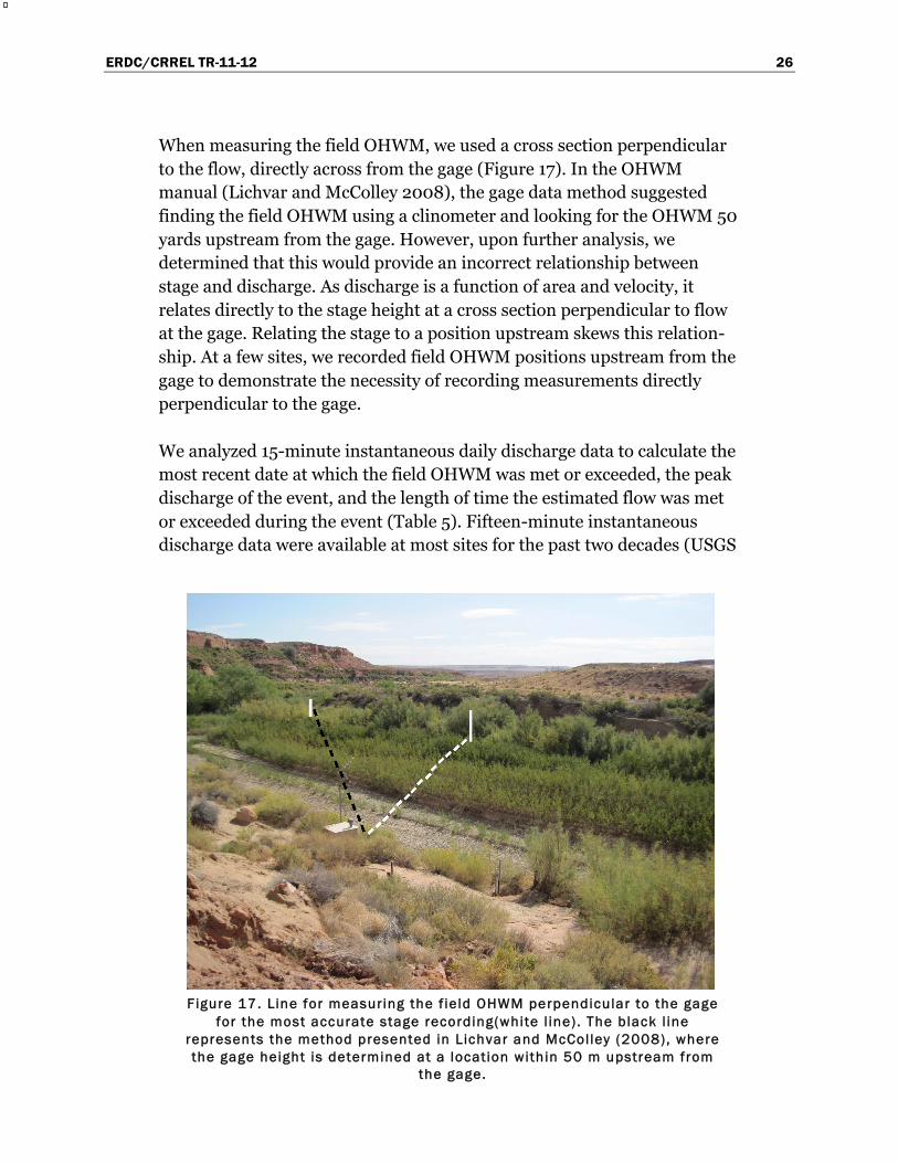
When measuring the field OHWM, we used a cross section perpendicular to the flow, directly across from the gage (Figure 17). In the OHWM manual (Lichvar and McColley 2008), the gage data method suggested finding the field OHWM using a clinometer and looking for the OHWM 50 yards upstream from the gage. However, upon further analysis, we determined that this would provide an incorrect relationship between stage and discharge. As discharge is a function of area and velocity, it relates directly to the stage height at a cross section perpendicular to flow at the gage. Relating the stage to a position upstream skews this relation-ship. At a few sites, we recorded field OHWM positions upstream from the gage to demonstrate the necessity of recording measurements directly perpendicular to the gage.

We analyzed 15-minute instantaneous daily discharge data to calculate the most recent date at which the field OHWM was met or exceeded, the peak discharge of the event, and the length of time the estimated flow was met or exceeded during the event (Table 5). Fifteen-minute instantaneous discharge data were available at most sites for the past two decades (USGS

Figure 17. Line for measuring the f ield OHWM perpendicular to the gage

for the most accurate stage recording(white l ine). The black l ine represents the method presented in Lichvar and McColley (2008), where the gage height is determined at a location within 50 m upstream from

the gage.


2009), although data for the days with higher flows were often missing, particularly for sandy bed channels such as Mission Creek, Cristianitos Creek, Palm Canyon, and New River. Fifteen-minute instantaneous discharge data refers to the discharge converted from the stage height recorded every 15 minutes; when flow is sporadic, the 15-minute instantaneous record has poor accuracy (greater than 20% of true discharge) and it is considered too unreliable to use. The more complete record of daily mean discharge data often does not capture the flashy peak precipitation events (Figure 12), but is an average of the 15-minute instantaneous measurements for the day. As high flows are short duration, lasting only a few hours, the daily mean discharge often is biased by lower flows and do not represent the geomorphically effective event. At sites where hourly data were collected for a short period, we interpolated the results to develop a more complete 15-minute record. However, if data were missing for more than 2-hour periods, we excluded the time from the analysis to prevent missing a flashy precipitation event. We performed this detailed analysis for the year of the gage-predicted ordinary high flow and the following years. The percentage of data missing from this period is listed for each site to demonstrate the possible limitations of using this instantaneous data record (Table 5). Additionally, we calculated the cumulative number of hours the field OHWM was exceeded in the past year, the past decade, and the past two decades (Table 5) to determine if there is a frequency component to developing an OHW signature. Peak days were missing from many sites, so this estimate is likely conservative.


Table 5. Percentage of days missing since the last gage-predicted ordinary high f low and the cumulative number of hours the f ield OHWM was exceeded in the past year, past decade,

and past two decades.

Most recent event exceeding the field OHWM

Cumulative # hrs field OHWM exceeded in the past

River Name

% Missing Record Date

Peak Discharge (cfs)

Stage (ft)

# Hrs Exceeded Year Decade

Two Decades

Rio Puerco 2.42% 8/10/2006 6210 19.52 Unknown 0 21.25 21.25 10/7/2006 3080 17.90 1 0 21.25 36.75 Moenkopi

Wash 13.94%

7/23/2007 2690 17.30 0.5 0 35.25 55.75

Dry Beaver Creek*

1.66% 12/7/2007 9600 9.30 4.75 0 8.5 52.0

Agua Fria River

3.33% 1/28/2008 14300 17.70 4.75 0 71.0 179.5

New River 0.34% 12/26/2008 3180 6.20 4.5 4.5 101.5 249.25

Hassayampa River

43.16% 2/12/2005 14500 13.70 0.25 0 0.25 5.25

Mission Creek†

4.15% 0 0 0

Palm Canyon†

10.67% 0 0.25 21.5

Cristianitos Creek**

0.53% 1/11/2005 3500 12.01 8.25 0 8.25 n/a

Deer Creek 3.4% 6/7/2009 18 2.95 10.75 1971.25 32627.75 64355.75

3/4/2009 1230 5.15 17.5 23.5 728.25 2367.25 Black Creek 1.31% 3/4/2009 1230 5.15 11.5 16.5 589.75 1982.0 4/7/2006 1830 6.09 7.5 0 60.0 90.75 Rock Creek†† 15.58% 4/7/2006 1830 6.09 90.5 0 291.75 369.5

Note: Mojave and Santa Maria are not included because they lack a field OHW signature. * During the flood recession at Dry Beaver Creek, the flow hovered around the field OHWM for 8 hrs. † Larger discharge events are missing from the record. ** Data at Cristianitos Creek were only available from 1993. †† The percentage of days missing data at Rock Creek is related to ice affecting the flow during the winter months. During the 4/7/2006 flood recession, the flow was around 1250 cfs (5.45 ft) for 1 day, approximately 130 cfs (0.15 ft) higher than the field OHW.


6 Results

6.1 Instability in the stage–discharge relationship

One of the main challenges in developing a consistent and reliable stage–discharge relationship for ephemeral and intermittent channels in the Arid West is the frequently changing channel characteristics. Many of these channels are dynamic systems where the channel morphology is unstable and ordinary high events result in a geomorphically effective event. The channel roughness, the resistance to flow, is constantly changing when vegetation on the active channel is removed by OHW events and subse-quently becomes re-established within a few years after the flood. The dominant sediment clast size may vary within a channel as low flows deposit sediments along the channel bottom at locations where the fine sediments were removed during larger floods. Photographs dating from 2003 to 2009 at three sites (Mission Creek, Mojave River, and New River) document these phenomena well.

Figure 18 shows the changes in channel morphology and vegetation cover at Mission Creek after a low to moderate flood (4.1-year recurrence interval) and a moderate to high flood (13.7-year recurrence interval). Figure 19 shows the annual peak flood and both the daily mean discharge (Figure 19A) and the 15-minute instantaneous discharge (Figure 19B) for the past decade. Note that, for the daily mean and 15-minute instantane-ous discharges, the recorded discharge is often missing or lower than the annual peak flood. These peak flood events are of such short duration that it is challenging to collect an accurate discharge measurement. Because of the uncertainty in stage–discharge relationships, the instantaneous peak discharge may be estimated from high flow indicators; thus the accuracy of the data point is limited and may not be included in the record.

In September 2003, after 5 years of low flows with recurrence intervals of less than 1.5 years, the vegetation was well established across the channel at Mission Creek and there was a gradual break in slope, possibly indicating the outer extent of the OHWM (Figure 18A). In January 2005, a 4.1-year flood removed the vegetation and created a sharp break in slope where sediment was eroded from the bank on the right side of the channel, clearly defining the OHWM (Figure 18B). Between this slope break and the


confining mountain, the channel cross section was relatively flat. The July 2009 photograph shows that the 13.7-year flood of 20 July 2008 appeared to stay within the active channel established by the 2005 flood, but it deeply incised the middle portion of the channel (Figure 18C). With this channel erosion, the channel cross section significantly changed, lowering the GZF and altering the stage–discharge relationship. Thus, the rating curve for Mission Creek has been developed from only a couple of site visits within the year since the flood reshaped the channel morphology. Because of the lack of data, the accuracy of the stage–discharge relation-ship is greatly limited at the rare moderate to high flows.

Figure 18. Changes in channel morphology and vegetation at Mission Creek: (A) September 2003 after 4 years of low f lows, (B) February 2005, 1 month after a 4.1-year f lood, and (C)

July 2009, 1 year after a 13.7-year f lood.


Figure 19. Flood hydrographs for the last decade at Mission Creek, showing the annual peak f lood (diamonds) and (A) dai ly mean discharge and (B) 15-

minute instantaneous discharge. The annual peak f lood and dai ly mean discharge are from the USGS Water Resources National Water Information

System (http://waterdata.usgs.gov/nwis/rt) and the instantaneous discharge is from the USGS Instantaneous Data Archive (http://ida.water.usgs.gov/ida).

A

B


The Mojave River also demonstrates the effect of a moderate–high flood on a channel when the vegetation and channel hydraulic roughness is changed (Figure 20). The discharge record for the past decade is shown in Figure 21. Although it is challenging to observe the changes to the channel morphology from photographs at a tributary junction and a view looking

Tributary Junction Downstream

Figure 20. Changes in channel morphology and vegetation at Mojave River: (A) September

2003 after 4 years of low f lows, (B) July 2005, 6 months after a 20-year f lood, and (C) July 2009 after 4 years of low f lows.

B

C

A


downstream on the Mojave River, the vegetation changes in the channel are pronounced (Figure 20). In September 2003, after 4 years of low flows with recurrence intervals of less than 2 years, vegetation has become well established in the channel (Figure 20A). The 20-year flood in January 2005 reworked the channel, removing all vegetation and subsequently reducing the channel resistance to flow (Figure 20B). Four years later

Figure 21. Flood hydrographs for the last decade at Mojave River, showing the annual peak f lood (diamonds) and (A) dai ly mean discharge and (B) 15-minute

instantaneous discharge.

B

A


without a moderate to large event, the vegetation has become re-established within the channel and the channel hydraulic roughness has increased (Figure 20C). These changes to the channel bed impact the rate at which water flows through the channel, which in turn alters the stage–discharge relationship.

A third phenomenon affecting the stage–discharge relationship is demonstrated at New River, where the dominant sediment size changes as erosion or sedimentation processes rework the channel morphology (Figure 22). The flow dynamics for the past decade at New River are shown in Figure 23. Following a 24-year flood in July 2005, cobbles dominated the channel sediment size (Figure 22A). Very fine sediments surrounded the cobbles. In September 2009, sand-sized sediment had been deposited around and over the cobbles from a 4.8-year flow in January 2008 or the subsequent low discharges in the past year (Figure 22). This sand has likely raised the relative elevation of the channel cross section, altered the roughness of the channel, and impacted the stage–discharge relationship.

Upstream to gage Downstream

Figure 22. Changes in channel morphology and vegetation at New River: (A) August 2006,

1 year after a 24-year f lood, and (B) September 2009, 1.5 years after a 4.8-year f lood.

B

A


Figure 23. Flood hydrographs for the last decade at New River, showing the annual peak f lood (diamonds) and (A) dai ly mean discharge and (B) 15-minute

instantaneous discharge.

B

A


6.2 Comparison between the field and gage-predicted OHWM recurrence intervals

In this study, we found that the field OHWM was consistently located at a lower stage than the stage of the gage-predicted ordinary high 5- to 10-year discharge (Table 4). This relative position of the field OHWM was consistent across a wide range of channel morphologies from wide, shallow channels to narrow, incised channels and a wide range of active channel sediment textures from sand to large boulders to bedrock. With the variability of the channel morphology, drainage areas, climates, and hydrologic conditions (Table 2), the frequency and duration of an ordinary high flow for a particular channel is unpredictable. Recurrence intervals for the field OHWM range from <1 to 15.5 years (Table 4), and the cumulative number of hours the OHWM flows have been met or exceeded over the past two decades varied from 5.25 to 64,355.75 hours (7.34 years) (Table 5). Below, photographs of each site and the locations of the field OHWMs are shown and described to provide an understanding of the variation of channel characteristics and OHW recurrence intervals in ephemeral and intermittent streams throughout the Arid West region. Additionally, the percentage of time the flow is exceeded and possible events that may align with the field signature are listed where applicable (Table 5).

An example of the variation in gage and field OHWMs is well documented in ground (Figure 24) and aerial (Figure 25) photographs of Mission Creek. Approximately 25 ft (7.6 m) upstream from the gage, the gage-predicted OHWM is approximately 1.3 ft higher in stage than the field OHWM (Figure 24). There was not a clear OHWM signature present directly perpendicular to the gage because a new pipe had recently been installed in the channel. However, if the field and gage-predicted OHWM were measured at the gage, the stage of the field OHWM would be even lower than the gage-predicted OHWM because of the slope of the water surface. The field OHWM is located at a position on the channel bank where there is a sharp change in sediment texture and a break in slope. Above this field boundary, the vegetation is more established and there are no drift indicators present. Conversely, no OHWM indicators are linked to the gage-predicted OHWM. Its position is partway up the slope before the bank flattens to a level floodplain, and the sediment texture and vegetation characteristics are the same above and below the gage-predicted boundary.


Figure 24. OHWM at Mission Creek: (A) field OHWM shown

by the break in slope, change in sediment texture, and change in vegetation successional stage, and (B) gage-

predicted OHWM with no indicator changes.

Figure 25. Aerial v iew of Mission Creek showing the posit ion of GPS points col lected. Point 1 l ies at the f ield OHWM; Point 2 is the gage-predicted OHWM. Blue circles are posit ioned along the f ield OHWM;

yel low circles represent the posit ion of the gage-predicted OHWM; the white circle is the gage; the green arrows point to the f ield OHW

signature. The blue arrow points in the direction of f low.


This field and gage-predicted OHWM variation is also visible in the aerial photograph of Mission Creek (Figure 25). Point 1 corresponds to the field OWHM shown in Figure 24A, while point 2 is equivalent to the gage-predicted OHWM in Figure 24B. Points 3, 4, and 5 were collected along the field OHWM signature and correspond to stages of 6.0, 6.9, and 9.6 ft, respectively. Note on the aerial photograph a slight darkening in pixel color marking; this boundary shown by the green arrows. In the field, this line is characterized by a change in sediment texture and a break in slope. Points 3 and 6 correspond to the gage-predicted OHWM, a stage of approximately 6.0 ft. At point 3, 86 ft (26 m) upstream from the gage, the field and gage-predicted OHWM signatures align. Point 6, 207 ft (63 m) upstream from the gage, is positioned at the top of the current low-flow channel. In Figure 25, the darker middle channel represents water flowing within the low-flow channel at the time the photograph was taken, corresponding with the position of the low-flow channel observed in the field. The positioning of the gage-predicted OHWM demonstrates how, across from the gage, the gage-predicted OHWM is higher than the field signature but is lower farther upstream at Point 6. The field OHW signature stage changes with the slope of the channel bed; the gage-predicted OHW stage is the same, thus representing different floodplain units of the channel farther upstream from the gage.

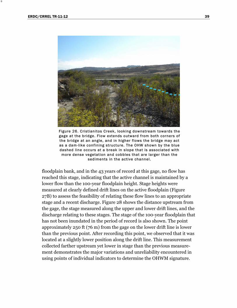
At two other channels, Cristianitos Creek and Santa Maria River, the OHWM was also determined upstream from the gage. At Cristianitos, a bridge over the channel likely acts as a dam during higher flows (Figure 26). The field OHWM was 3.5 ft lower in stage than the gage-predicted OHWM. This field OHW stage height has not been reached since the gage-predicted OHW flood in 2005. This field OHWM corresponds to a recurrence interval of 4.9 years, and the primary indicator was a change in vegetation cover between the active channel and the 100-year floodplain. Farther upstream from the dam, a more defined OHWM was associated with a cluster of cobbles at the boundary and an increase in the density of the vegetation. Three stage heights were collected upstream from the gage along the field OHWM. At approximately 325 ft (99 m) above the gage, the field OHWM was still almost 2 ft lower than the gage-predicted OHWM.

The field OHW stage could not be determined at Santa Maria because there was no OHW signature at the gage. Directly across from the gage, the active channel had eroded into the 100-year floodplain bank, exposing tree roots (Figure 27A). The stage was measured at the top of the 100-year


Figure 26. Crist ianitos Creek, looking downstream towards the gage at the bridge. Flow extends outward from both corners of the bridge at an angle, and in higher f lows the bridge may act as a dam-l ike confining structure. The OHW shown by the blue dashed l ine occurs at a break in slope that is associated with more dense vegetation and cobbles that are larger than the

sediments in the active channel.

floodplain bank, and in the 43 years of record at this gage, no flow has reached this stage, indicating that the active channel is maintained by a lower flow than the 100-year floodplain height. Stage heights were measured at clearly defined drift lines on the active floodplain (Figure 27B) to assess the feasibility of relating these flow lines to an appropriate stage and a recent discharge. Figure 28 shows the distance upstream from the gage, the stage measured along the upper and lower drift lines, and the discharge relating to these stages. The stage of the 100-year floodplain that has not been inundated in the period of record is also shown. The point approximately 250 ft (76 m) from the gage on the lower drift line is lower than the previous point. After recording this point, we observed that it was located at a slightly lower position along the drift line. This measurement collected farther upstream yet lower in stage than the previous measure-ment demonstrates the major variations and unreliability encountered in using points of individual indicators to determine the OHWM signature.


Figure 27. Channel characterist ics at Santa Maria: (A) View across the stream from the gage—Note the eroded bank on the far shore and the numerous point bars with coarser

sediments throughout the channel. (B) View upstream—Drift l ines showing high water marks from a previous f lood are accumulated on the point bars. The upper drift l ine is indicated by

the green arrow; the lower drift l ine is indicated by the blue arrow.

Figure 28. Stage along drift l ines and the 100-year f loodplain for Santa Maria.


The Mojave River is another example of a channel lacking a well-developed active floodplain directly at the gage (Figure 29). One bank is restricted by a riprap-supported railroad track, and the other bank is confined by a mountainside. Except for low flows that migrate throughout the channel, the channel is incised such that water flows across the entire channel between the banks for most discharges. As there are no active floodplains or 100-year floodplains at the gage, there is no clear OHW signature to use in assessing the accuracy of the stage–discharge relationship at this site.

Figure 29. Gage at Mojave River, located beneath the rai lroad tracks. The channel f lows between the r iprap-supported rai lroad track banks and the mountainside.

Rio Puerco is an incised channel where most of the flows remain within the channel banks (Figure 30A). In 2006, the largest flood in the past 30 years occurred. This flood has a recurrence interval of 5.4 years, as determined from the 70 years of record at Rio Puerco. Its field signature is clearly visible on the channel bank as a sharp break in slope (Figure 30B) and aligns with the gage-predicted stage of 19.52 ft. However, the recent changes in flow conditions at Rio Puerco suggest that this event no longer relates to the ordinary high flow (Figure 31). The annual peak flows have decreased substantially over the past three decades. The field ordinary high flow under the climate conditions of the past 30 years has a recur-rence interval of 15.5 years (2.9 years over the full period of record). It is identified by a break in slope and a change to more established vegetation above the boundary. This stage has not been reached since the peak event in 2006 and cannot be related to a recent event.


Figure 30. Channel characterist ics at Rio Puerco: (A) Most f lows remain within the deeply incised channel banks. The f ield OHWM is shown by the blue dashed l ine. (B) In 2006, the largest f lood in the past 30 years left a clear signature showing its outer extent, shown by

the yel low dashed l ine.

Figure 31. Annual peak streamflow at Rio Puerco. The dashed l ine shows

the approximate t ime when peak f lows were reduced signif icantly.


Moenkopi Wash is an incised channel with OHW signatures on each bank, an eroded sand bank across from the gage, and a sparsely vegetated bedrock outcrop on the bank where the gage is located (Figure 32). On the sand bank, the field OHW signature is clearly defined by a sharp change in vegetation composition and successional stage. There is also a break in slope directly at this vegetation transition. The gage-predicted OHWM stage (20.5 ft) for the 4.5-year flow is 4 ft above this field OHW signature (16.6 ft). On the bedrock bank on the gage side of the channel, the field OHWM is 1 ft higher (17.6 ft) than the field OHWM on the sand bank. Above the break in slope at the field OHWM on the bedrock bank, sages (Salvia sp.), an upland species, are established, and there is no drift or signs of flowing water. The field OHWM recurrence intervals are 1.5 and 1.6 years for the sand bank and bedrock bank, respectively. The field OHWM on the sand bank does not align with a recent flow. However, the gage-side bank may relate to two events: a flow 0.3 ft lower than the field OHW stage on 23 July 2007 and a flow 0.3 ft higher on 7 October 2006 (Table 5).

Figure 32. Moenkopi Wash, with the f ield OHWM shown by

the blue dashed l ines. Note the clear changes in vegetation successional stage from the low-f low channel

with no vegetation to the active channel with early successional stage vegetation to the 100-year f loodplain

with establ ished late-stage vegetation.


Palm Canyon Wash is a sand-bed channel with a narrow floodplain (Figure 33A). The dominant feature defining the field OHWM is a break in slope (Figure 33B). Above this break in slope, there is an increase in vegetation cover and a lack of drift. The field recurrence interval is 4.6 years. Fifteen-minute instantaneous peak flow data are missing for Palm Canyon Wash, so a frequency of flows that meet or exceed the field OHWM could not be determined.

Figure 33. Palm Canyon Wash, with the f ield OHWM shown

by the blue dashed l ine: (A) v iew upstream towards the gage, and (B) eroded slope below the f ield OHWM.


The low-flow channel at New River has no vegetation cover and is dominated by sand-sized sediment (Figure 34A). The active channel is characterized by multiple benches that have cobble textures along the bench slope and vegetation established at the break in slope on top of each bench. The field OHWM is identified from these minor benches by a more distinct shift to late-stage vegetation and a fining of the dominant sediment size above the break in slope (Figure 34B). This field OHWM has a recurrence interval of 1.7 years and does not relate to a recent flow event. In 2008 the recent flow event peaked at a stage of 1.4 ft above the field OHWM.

Figure 34. New River, with the field OHWM shown by the blue dashed line: (A) View perpendicular to the gage. The

field OHWM is located at the third row of shrubs in the back-ground. (B) Field OHWM, defined by a change in sediment

texture, a break in slope, and late-stage vegetation.


Figure 35. Agua Fria, with the f ield OHWM shown by the

blue dashed l ine: (A) v iew from a cl i f f overlooking the channel, and (B) photo at the location shown by the arrow in A looking downstream shows the cobble-bed dominated active channel with denser vegetation above the OHWM.

The cottonwoods on the r ight al ign with the low-f low channel banks.

The field OHWM at Agua Fria is also below the gage-predicted OHWM. Figure 35A, a view from a cliff overlooking a channel, shows water in the low-flow channel and a sparsely vegetated active channel. The extent of the field OHWM aligns with a break in slope, denser vegetation, and a change in sediment texture with an absence of boulders above the OHWM (Figure 35B). The field OHWM has a recurrence interval of 2.7 years and is


2 ft below the most recent high flow event in 2008. The low-flow channel is positioned between two cottonwood banks at the gage, and the channel bed is dominated by fine-grained sand. Based on the instantaneous 15-minute discharge record, the majority of flows remain within this low-flow channel, with only 0.9% of the flows in the past two decades extending beyond the cottonwoods onto the active cobble channel.

The field OHWM at Dry Beaver Creek lies at a break in slope, about 1 ft above the extent of the cobble bank. Although a challenge to see in Figure 36, the boundary aligns with the establishment of vegetation and a shift to fine-grained sediments. Fifteen-minute instantaneous discharge data suggest that this field OHWM boundary is rarely reached, with approxi-mately 52 hours of flows greater than the field OHWM over the past two decades. However, this field OHWM boundary aligns closely with the flood recession of the 5.4-year 2007 gage-predicted ordinary high flow. During the flood recession, the flood remained within 1,000 cfs (0.3 ft) of the field OHWM for 8 hours. The gage-predicted OHWM from the 2007 flood lies 2 ft above this field boundary. There is no break in slope or change in vegetation at the gage-predicted OHWM. The second gage-predicted OHWM, the 9.8-year flood in 2004, lies at the top of the 100-year floodplain, 6 ft above the field-predicted OHWM.

Figure 36. Channel characterist ics at Dry Beaver Creek: The f ield OHWM is shown by the blue dashed l ine, and

the gage-predicted OHWM from the 5.4-year f lood in 2007 is shown by the yel low dashed l ine.


Figure 37. Channel characterist ics at Black Creek: (A) gage-predicted OHWM, and (B) f ield

OHWM signature shown by the blue dashed l ines. The approximate location of the outer bank of the gage-predicted OHWM is shown by a yel low l ine in the background and al igns

with the extent of the stadia rod shown in A.

At Black Creek, the gage-predicted OHWM is on the gently sloping outer banks of the channel (Figure 37A). During large events, the flow rises higher on the gradually sloping banks. The low-elevation floodplain at Black Creek is inundated annually and there are no 100-year floodplains. The field OHWM is identified by the minimal vegetation cover and the cobble bed of the active channel (Figure 37B) and has a recurrence interval of 1.1 years. This field signature does not align with a recent flow event. In March 2009, a 1,230-cfs flood occurred with a stage of 5.15 ft. This is significantly higher than the field OHWM stage of 3.5 ft that corresponds with a discharge of 140 cfs. The March 2009 flood inundated the entire channel width, covering the low floodplain. However, there were no apparent high water mark indicators along either bank from the 2009 flood. Post-flood, the discharges have not met or exceeded the field OHWM.

Deer Creek is a narrow, 20-ft-wide channel with large boulders in the active channel (Figure 38A). The banks are thickly vegetated and branches overhang the channel, trapping significant drift. The field OHWM is located at a break in slope above the large boulders, and the recurrence interval for the field OHWM is less than 1 year. Vegetation becomes well-established beyond this break in slope, as seen in Figure 38B. This field OHW stage has been exceeded for a total of 82 days in the past year. The


Deer Creek watershed extends into the extent of the Corps-defined Western Mountains, Valleys, and Coast Region, so it is possible the different characteristics of the mountain channels may be influencing flow dynamics at this site.

Figure 38. Deer Creek, with the f ield OHWM shown by the

blue dashed l ine: (A) Active channel. The water l ine visible on the rocks is common to many of the boulders in this channel. (B) Establ ished vegetation on the slope above the OHWM. The boulders shown in A are covered

in this view by water.


Figure 39. Rock Creek, with the f ield OHWM shown by the

blue dashed l ine. The f ield OHWM is located where the bank slope becomes steeper and the vegetation changes.

Rock Creek is different from most channels in this study in that it has a bedrock bed at the gage (Figure 39). The field OHWM is defined by a steepening of the channel bank and a change in vegetation from grasses to shrubs. Above the OHWM, there are more fine-grained sediments present than in the channel, where bedrock and cobbles dominate. The field OHWM on the far bank highlighted in Figure 39 has a recurrence interval of 4.4 years. The field OHWM on the gage bank has a recurrence interval of 5.5 years, and its dominant indicator is a break in slope. On both banks, the gage-predicted OHWM is located at a position where similar vegetation, sediment texture, and slope angle can be found above and below the gage-predicted boundary. The field OHWM on the steep gage bank aligns within 0.09 ft of a flood on 7 April 2006; the field OHWM on the far bank is not associated with any recent events.

Hassayampa River is a sandy channel that flows through a straight confining reach at the gage (Figure 40A). Because flow stays between the bedrock outcrop and railroad track banks, there are not well-developed floodplain features. In this instance, the use of gage data to delineate the OHWM is helpful. As there are numerous flow indicators at varying elevations along the vegetated railroad bank, it is helpful to determine the OHWM by aligning the gage-predicted stage with the limited indicators available. The gage-predicted OHWM aligned with a minor break in slope and a vegetation change that represent the field OHWM (Figure 40B).


Above the OHWM, shrubs are well established, while below the OHWM, early to mid-successional vegetation is present. The recurrence interval for the ordinary high flow at Hassayampa is 8.8 years.

Figure 40. Hassayampa River, with the f ield OHWM shown by the blue dashed l ine: (A) channel confined by bedrock

outcrops on the left bank and a rai lroad track on the r ight bank, and (B) vegetation below the rai lroad track,

showing the sl ight increase in bank slope just below where shrubs are establ ished along the channel bank.


7 Discussion

7.1 Finding the OHWM from gage data: perpendicular to the gage versus upstream from the gage

In the 2008 Lichvar and McColley manual, the gage-predicted OHWM was related to a field OHWM signature within 50 yards upstream from the gage. However, using a position upstream from the gage can skew the stage–discharge relationship because discharge is the amount of water flowing through a given area, or cross section, during a particular time (Figure 9). Since the area is calculated perpendicular to flow, relating a stage height to a position upstream on the channel bank does not accurately capture the cross-sectional area because the stage height relates to a water surface elevation at the gage based on relationships derived using the cross-sectional area perpendicular to flow at the gage. Therefore, the estimated position of the gage-predicted OHWM is incorrect when measured upstream from the gage. The slope of the water surface and any change in channel morphology from the upstream position to the gage must be considered. Our results demonstrate that it is unreliable to link the stage to a location upstream from the gage without extensive channel surveys, which are beyond the scope of this study. Data points at Mission Creek, Cristianitos, and Santa Maria, all collected above the gage, demon-strate the unreliability of using the stage height of a recent event to esti-mate a discharge upstream from the gage.

At Mission Creek, GPS points were collected upstream from the gage at the field OHWM and gage-predicted OHWM (Figure 25). The field and gage-predicted OHWM aligned at 86 ft (26 m) upstream from the gage. The gage-predicted OHWM 207 ft (63 m) above the gage aligned with the current low-flow channel. Conversely, at Cristianitos, the gage-predicted OHWM was approximately 2 ft higher than the field OHWM 350 ft (107 m) above the gage. This variation between sites and ordinary high-flow field signatures was a consistent theme throughout this study. It is misleading to choose a set distance upstream from the gage where the gage-predicted and field OHWMs would be expected to align. At Mission Creek, the field OHWM is below the gage-predicted OHWM 50 yards above the gage, while at Cristianitos, the field OHWM is higher. The only consistent method is to compare the field and gage-predicted OHWMs directly across from the gage.


Another challenge with finding the OHWM upstream from the gage is related to channel narrowing. At Cristianitos, the gage is located at a bridge, and the active channel narrows from 90 ft (27 m) wide 120 ft (37 m) above the gage to 45 ft (14 m) at the gage. The stage of the 8.0-year flood in 2005 was located at the top of the bridge; to reach that stage, water was restricted by the bridge (Figure 26). Water behind this bridge “dam” has a lower velocity than in an unrestricted channel because of a backwater effect, so the field signature of the ordinary high flow may not accurately reflect the true OHW event.

At Santa Maria, there is no active floodplain or OHWM signature at the gage because of channel narrowing. Drift lines on a point bar located approximately 75 ft (23 m) upstream from the gage (Figure 28) provide indicators that may be possible to relate to recent floods by assuming that the slope of the drift line relates to the slope of the water surface during the recent event. Since only one data point was collected along the upper drift line, we could not relate this indicator to a recent event. For the lower drift line, if a stage height is estimated at the gage from the slope of the three data points, the stage height should be 5.33 ft, corresponding to a discharge of 6,350 cfs. On 27 January 2008, this stage was exceeded by a flood event that peaked at 7,230 cfs, a stage of 5.65 ft. However, the third point appeared visually to be at a slightly lower position in the drift line and was at a lower stage height than the second point (Figure 28). Using only the first two points, we estimated the stage height to be 3.85 ft, corresponding to a discharge of 2,840 cfs at the gage. On 26 December 2008, a flood event peaked at 2,820 cfs, a stage of 3.83 ft, aligning closely with the first two data points. However, without more data points, we cannot determine the exact flow responsible for depositing the drift.

This method assumes that the slope of the drift line relates to the slope of a recent flood event and is the same slope at the gage as along the point bar. The two different predicted stage heights and related recent events at Santa Maria demonstrate the challenges of using individual indicators to predict a discharge event. Additionally, the drift line is located at a rela-tively wide portion of the channel. The point farthest upstream, 300 ft (91 m) from the gage, is located where the channel is 500 ft (152 m) wide. At the gage, there is a single channel that is only 300 ft (91 m) wide. As the channel narrows, the water surface slope most likely changes to accommo-date the change in channel cross-sectional area. This change in slope makes it impossible to estimate the true stage at the gage to determine a discharge, recurrence interval, and date of flow related to this drift line.


If points upstream from the gage are used to determine the discharge and recurrence interval of the OHW, extensive channel surveying must be conducted to determine how flow dynamics related to channel widening, channel narrowing, or flow restriction change from the gage to the point upstream from the gage. However, because of the large uncertainties in using gage data, it is better to observe the stage of the OHWM directly perpendicular to the gage.

7.2 Instability in the stage–discharge relationship

The accuracy of the stage–discharge relationship is one of the key factors to the usefulness of gage data. Each discharge value is estimated from rating curves, developed from a few measurements that relate stage to discharge. With flashy floods, shifting channel morphologies, changes in the hydraulic roughness, and long-term climate or land use changes, the accuracy of flow data for ephemeral and intermittent streams is limited. These instabilities related to a shifting stage–discharge relationship over time must be acknowledged and considered when using gage data from ephemeral and intermittent streams.

One of the challenges in developing an accurate stage–discharge relationship is the flashiness of ephemeral and intermittent systems. Velocity measurements at each vertical segment should represent 5% or less of the total flow, requiring that 25–30 verticals be collected for each discharge measurement (Sauer and Meyer 1992). For flashy storm events where peak discharges are reached and passed quickly, the time required to collect 25–30 verticals makes it nearly impossible to capture the true discharge. When measurements are collected, the discharge and stage likely change from the start of collection to the end. Thus, the highly uncertain indirect measurements (Sauer and Meyer 1992, Tillery et al. 2001) from high water marks are often the best option for relating stage to discharge for moderate to large events.

Previous research has demonstrated that the stage–discharge relationship can change during a storm, with the increasing discharge behaving differently than the receding flow (Lohani et al. 2006, Shrestha and Simonovic 2010). This hysteresis causes the same stage to have a higher discharge during the rising flood than during the receding flood (Lohani et al. 2006). These changes within a single storm event, magnified by the constantly shifting channel morphology of ephemeral and intermittent


streams, make it particularly challenging to develop an accurate stage–discharge relationship.

Sandy-bed channels such as Mission Creek (Figure 18) experience the majority of aggradation and degradation of river systems. These desert rivers have extremely high sediment transport rates compared to perennial streams because of the readily available material from the poorly vegetated slopes and the often sandy channel beds (Reid and Frostick 1997). In a study of discontinuous ephemeral streams, Bull (1997) found sediment dynamics similar to those we observed at New River (Figure 22), where low to intermediate flows aggraded the channel while higher flows scoured the channel. The constant shifts in channel morphology make it challenging to establish a stage–discharge relationship, limiting the availability of gage data for these sandy ephemeral and intermittent streams.

Channels with cobble or boulder-size sediment in the active channel, such as Dry Beaver Creek, respond differently to flow events than sand-bed channels. Cobble-bed streams are fairly stable during low to moderate flows, but large events are capable of transporting large amounts of bedload material (Tillery et al. 2001). The low-flow channel in these systems migrates after an OHW to high flood event transports the large rocks on the bed but does not aggrade and erode as frequently as the low-flow channel in sand-bed channels.

The frequent changes in bed sediment size and vegetation growth and removal (Figures 18 and 20) alter the channel bed’s hydraulic roughness. The hydraulic roughness affects the stage–discharge relationship by influencing the channel’s resistance to flow. As a channel’s resistance to flow increases, the velocity of flow decreases, so a particular discharge has a higher stage. Large clast size and less uniform sediment distribution and vegetation growth increases the hydraulic roughness (Bull 1997, Tillery et al. 2001, Nolan et al. 2008). At Mission Creek (Figure 18) and Mojave River (Figure 20), the vegetation is removed by larger events and becomes established during lower flows, requiring frequent adjustments to the stage–discharge relationship.

The stage–discharge relationship is altered significantly over longer periods of time by land use and climate changes. At Rio Puerco, the channel has incised and abandoned floodplain surfaces (Phippen and


Wohl 2003) such that the 100-year floodplain inundated by the large event in 2006 was likely once the active floodplain. Climate change throughout central New Mexico has resulted in an increase in the total annual precipitation but a decrease in the annual peak flow at Rio Puerco (Molnar and Ramirez 2001, Pelltier 2006). The 2006 flood had a recurrence interval of 5.4 years; however, it was the largest event in the past 30 years (Figure 31). Thus, under current climate conditions, the discharge does not correspond with an ordinary high event. In these dynamic ephemeral and intermittent systems that have been significantly altered by anthropogenic influences, changes in flow regime and channel morphology are likely and must be considered when analyzing flow dynamics.

However, despite these limitations, ranging from errors related to measuring discharge in flashy systems to changes in channel morphology to longer-scale climate changes, the uncertainty regarding the accuracy of the stage–discharge relationship cannot fully explain the discrepancy between the gage-predicted OHWM and the field OHWM signature. In some instances, the gage-predicted OHWM approximately 5- to 10-year discharge and stage were over 90% and over 40% greater than the field OHWM discharge and stage, respectively, corresponding to differences in discharge of over 3,000 cfs and 4 ft in stage. Stage–discharge uncertainties may account for a portion of the discrepancy, but it is more likely that each channel is unique and that ordinary high flow frequency and duration are channel specific.

7.3 Recurrence intervals of the field OHW

Identifying the OHW recurrence interval for Arid West ephemeral and intermittent streams is desirable for many purposes including flow modeling, regulation, and development. Many people would like to apply the 1.5- to 2-year bankfull concept to OHW in the Arid West because when designing structures for flood control, for example, it is beneficial to know the frequency of an OHW event occurring. However, we found recurrence intervals for the field OHWM range from <1 to 15.5 years (Table 4) and have a similar large discrepancy for the percentage of time flows meet or exceed the OHWM (Table 5). The recurrence interval of the OHW signature varies between channel banks and between sites of close proximity. More stable channels and channels located closer to the western mountain region may have lower recurrence intervals than more sandy channels.


There is variation in the field OHW recurrence intervals between channel banks at the gages at Rock River, Moenkopi, and Black Creek. For example, the recurrence intervals for the banks at Rock River are 5.5 and 4.4 years, corresponding to a discharge of 1750 and 1120 and a difference in stage between banks of 0.7 ft. Similarly, at Moenkopi, one OHW signature on the channel bank is 1 ft higher than the field OHWM on the opposite bank. Black Creek, a wide, shallow, braided channel, has a difference of 0.1 ft. These variations demonstrate the limitations of applying a recurrence interval to an ordinary high flow, as differences occur in OHW stage due to changes in channel bank slope, substrate, and vegetation, even with a reliable, repeatable methodology to determine the field signature. At Moenkopi and Rock River, the steeper bank that does not have a floodplain had the higher stage and recurrence interval. It is possible that, without a 100-year floodplain on a bank, the characteristic OHW indicators of a break in slope and vegetation changes relate more to recent events that leave high water marks than to the signature created by the OHW event. At Moenkopi, on the steep gage bank, a flood peaked 0.3 ft below the stage of the field OHWM on 23 July 2007, and a flood peaked 0.3 ft above the stage of the field OHWM on 7 October 2006. At Rock Creek, on the steep gage bank, a flood peaked 0.1 ft about the field OHWM and remained between the peak stage and field OHW stage for 7.5 hours. This variation suggests that the channel characteristics impact the flow magnitude responsible for developing an OHW signature.

Additionally, one of the challenges in finding trends between flow datasets is that each channel is unique. Drainage area, location within the water-shed, and ecoregion appear to have minimal impact in defining what an ordinary high flow recurrence interval is for ephemeral and intermittent channels. The active floodplain for Aqua Fria is cobbles and boulders (Figure 35), while at New River, 5 miles (8 km) away, the active floodplain is sandy with a few small cobbles scattered along the bench slope (Figure 34). The recurrence interval is 2.7 years at Agua Fria and 1.7 years at New River. These channels are both confined on one bank by bedrock cliffs and are a gradual slope with floodplain and terrace benches to the hills on the other side. With different recurrence intervals for these two similar channels in close proximity, it is not surprising to find substantial differences throughout the Arid West, where the channels vary in geology, vegetation, and climate.


Despite these differences between Arid West ephemeral and intermittent streams, one trend is that higher recurrence intervals are associated with unstable, less-incised, sandier channels. Mission Creek, Palm Canyon, and Cristianitos flow through relatively unconsolidated material, and the recurrence intervals at these sites are 7.4, 4.6, and 4.9 years, respectively. Mission Creek, which is the least incised with the widest available floodplain, has the highest OHW recurrence interval. Conversely, channels with coarser substrates of cobbles and boulders, such as Black Creek, Agua Fria, New River, and Dry Beaver Creek (1.1, 2.7, 1.7, and 3.6 years, respectively), and incised channels with limited sediment available for transport, such as Moenkopi (1.6 years), have lower recurrence intervals. One exception to this trend is Rock River, with a recurrence interval of ~5 years. Rock River is a bedrock-dominated system with little sediment available for transport during high flows. The snowmelt-driven high flows in the spring are less flashy than at other sites in this study, where ordinary high flows are generally associated with instantaneous precipita-tion events. At Rock River, the OHWM is created and maintained by longer events than at many other Arid West streams. More research needs to be conducted to determine if snow-driven channels tend to have higher recurrence intervals.

Another trend is that sites located near the boundary between the Arid West region and the Western Mountain region, Deer Creek and Black Creek, have the lowest recurrence intervals in the study: less than 1 and 1.1 years, respectively. These channels are both located in the foothills and have Mediterranean climates. The substrates of the active channels in Deer Creek (Figure 38A) and Black Creek (Figure 37B) are different than most other channels in the study. The bed of the active channel is large boulders in Deer Creek and cobbles in Black Creek, with minimal fine-grained sediments within the active channel. Deer Creek almost meets the flow requirement for a perennial stream, and although there are dry periods in most years, flow is greater than 1 cfs for approximately 89% of the period of record. Deer Creek is narrower and more densely vegetated than other sites in the study, and there is not a well-developed floodplain. These characteristics, the proximity to the mountain region (6.1 miles), and the almost perennial flow may explain the low recurrence interval for the OHWM at Deer Creek.

Conversely, Black Creek has periods of no flow for almost half the year and has an extensive 100-year floodplain that is sandier than the active


channel. The 100-year floodplain at Black Creek is vegetated with similar grass species as the ancient terrace and demonstrates no indications that the area has flooded frequently. The ordinary high flow at Black Creek has a 1.1-year recurrence interval. Although its characteristics are possibly less common throughout the Arid West than the sandy, highly erodible channels like Mission Creek and Santa Maria, Black Creek meets the criteria of an ephemeral or intermittent channel in the Arid West region, with mean daily flows less than 1 cfs 64.7% of the time over the period of record. Its low recurrence interval is a result of what is “ordinary” to this channel.

7.4 Limitations of using gage data to define the OHW event

The wide range of OHW recurrence intervals from <1 to 15.5 years for sites in this study makes it unreliable to determine the OHW from gage data prior to visiting a site and examining the flow conditions. Additionally, the limited availability of gage data for Arid West ephemeral and intermittent streams often makes it challenging to determine the frequency of a particular event and what is “ordinary” to a channel. Using the gage-predicted ordinary high flow also resulted in the OHWM appearing to relate to multiple recurrence intervals over time at Mission Creek, based on photographic comparison. Because of these uncertainties, using physi-cal features to identify the OHWM is the most reliable and repeatable methodology. Gage data provide critical information about flow dynamics at a site and can assist in identifying a challenging OHWM boundary, but they cannot be used to define the highly variable OHWM.

In this study, we defined ordinary high flow as the most recent (within the past decade) low to moderate (~5–10 year) flood. Prior to visiting the sites, we selected the most recent OHW event from gage data. At Dry Beaver Creek, there were two events in the past decade that met the low to moderate criterion: the 5.4-year flood on 7 December 2007 and the 9.8-year flood on 29 December 2004. However, no flow indicators were present at the positions on the landscape for either of these floods. Instead, the OHWM field signature was lower, aligning with a 3.6-year flood. This trend was for the same at the other sites in this study, where the ordinary high flow we selected from gage data was greater than the discharge responsible for developing the field OHWM. Each ephemeral and intermittent Arid West stream has a unique ordinary high flow and recurrence interval that cannot be selected from gage data. Similarly, the field OHWM is often unrelated to recent flow events, and there is not a


required duration of flow to create and maintain the OHW signature (Table 5). The OHW field signature has been met or exceeded by flows from 5.25 to 64,355.75 hours (7.34 years) over the past two decades. This suggests that gage data cannot be used to determine the recurrence interval or recent flood event responsible for creating the signature.

Another consideration in using gage data to identify the ordinary high flow is that the recurrence interval calculation is less accurate for gages with shorter periods of record. For example, if only 10 years of data are available, the largest flood in that period will have a recurrence interval of only 11. However, if 50 years of data are available for the site, that same discharge may be the largest over the course of 50 years and have a recurrence interval of 51, or it may be a moderate event and statistically occur every 10 years. For example, at Rio Puerco during the past three decades, the annual peak flow has decreased to a lower magnitude discharge than during the previous years of data collection (Figure 31). The gage-predicted ordinary high flow has a recurrence interval of 5.4 years over the 70 years of record, but for the past three decades, the recurrence interval is 31 years. Similarly, Cristianitos Creek has only 16 years of data. The OHW event has a recurrence interval of 4.9 years, but as more data are collected, this recurrence interval may change. Thus, with limited data or changing flow conditions at many ephemeral and intermit-tent streams, it is often challenging to develop a true understanding of the magnitude and frequency of an ordinary high discharge at each site.

Photographic and gage data analysis suggest that the ordinary high flow may relate to more than one recurrence interval at a site over time. At Mission Creek, photographs suggest that the 4.1-year flood in 2005 created a strong active channel signature (Figure 18). Photos from 2008 suggest that the 13.7-year flood remained within the banks of the active channel created in 2005 but predominately eroded sediment from the channel by incision. As such, the recurrence interval related to the gage-predicted ordinary high flow at Mission Creek for the active channel may range from 4.1 to 13.7 years, depending on the date sampled. When we visited the channel in July 2009, the signature of the field OHWM corresponded to a recurrence interval of 7.4 years. These differences suggest that it may not be possible to assign a particular recurrence interval for OHW in Arid West ephemeral and intermittent streams as it may change over time.


However, for these Arid West streams, shifting channel morphologies limit the accuracy and availability of gage stations. Too few streams are undisturbed and gaged to allow us to accurately classify and determine the OHW recurrence interval for Arid West ephemeral and intermittent streams. Possibly the largest influence on the magnitude of flow needed to develop the OHWM is the channel morphology. Gages are typically built along stable channels with downstream controls to provide the best conditions to establish a stage–discharge relationship (Rantz 1982), so the majority of gaged sites throughout the Arid West are located in incised channels or confined reaches of the channel that may not be characteristic of most of the channels in the region. Of the 14 sites studied, 6 are located at or immediately upstream of bridges. The unique position of the gage may suggest trends in the channel regarding the recurrence interval of the OHWM that are uncommon. Sand-bed channels such as Hassayampa and Mojave are located between confining features such as bedrock cliffs and railroad tracks at the gage. Within a half mile below the gage, the confining banks end and the channel widens to a basin area with a wide active floodplain. Sediment processes at these sites change from strictly bed aggradation and incision at the gage to a reach with a dynamic active floodplain. Although gage data can be used only directly at the gage to determine a recurrence interval for ordinary high flows, it is possible that the recurrence interval varies with the channel morphology throughout a river. Extensive research beyond the scope of this study is needed to determine if the recurrence interval varies spatially within a channel.

One advantage to using gage data and knowing the gage-predicted stage and recurrence interval is that they can provide a general estimate for the magnitude of the most recent event flowing through the channel. At Hassayampa (Figure 40), the field OHWM was not as clear as at other sites because of the steep, incised channel banks and the lack of a 100-year floodplain. Knowing the gage-predicted 5- to 10-year OHW stage was useful at this site for locating the general position of the field OHWM on the channel bank.

Despite the unreliability of using the gage-predicted ordinary high discharge for identifying the OHWM, gage data provide critical information about flow dynamics. Gage data describe the recent flow conditions and provide information about how frequently a flood of a particular magnitude and stage flows through the channel. Understanding the overall flow regime for the channel is critical for any watershed study.


The lack of gages because of highly unstable channels and changes to the OHW recurrence intervals makes it important to have methods other than gage data to identify the lateral extent of the OHWM. The OHWM manual (Lichvar and McColley 2008) and supplemental datasheet (Curtis and Lichvar 2010) provide repeatable methodology for regulators to identify the lateral extent of the OHWM. Although we emphasize using field signatures to identify the OHWM, we recommend that users perform a flow frequency analysis (FFA) to develop an understanding of flow dynamics for a stream of interest.


8 Conclusion

This report supports Lichvar and McColley’s (2008) finding that using the field signature to identify the OHWM boundary between the active floodplain and 100-year floodplain is the most repeatable and reliable method. Most ephemeral and intermittent channels do not have gage stations because of the challenges in developing a stage–discharge relationship; a delineation procedure that relies on field indicators rather than flow data is a necessity. The potential errors in using gage data increase substantially in these unstable sandy Arid West channels, where the channel substrate shifts frequently and vegetation growth or removal leads to changes in hydraulic roughness. Recurrence intervals for the field OHWM range from <1 to 15.5 years, and there is no consistent frequency or duration of flow responsible for establishing and maintaining this field signature. This large variation and the limitations in developing a reliable stage–discharge relationship indicate that gage data are best used to describe flow dynamics for a stream and should not be used exclusively to identify the OHWM.


References Adams, D. K., and A. C. Comrie. 1997. The North American monsoon. Bulletin of the

American Meteorological Society 78: 2197–2213.

Bailey, R. G. 1995. Descriptions of Ecoregions of the United States. U.S. Forest Service. (http://www.fs.fed.us/land/ecosysmgmt/)

Bull, W. B. 1997. Discontinuous ephemeral streams. Geomorphology 19: 227–276.

Clemmens, A. J., and B. T. Wahlin. 2006. Accuracy of annual volume from current-meter-based stage discharges. Journal of Hydrologic Engineering 11: 489–501.

Curtis, K. E., and R. L. Lichvar. 2010. Updated datasheet for the identification of the Ordinary High Water Mark (OHWM) in the Arid West Region of the Western United States. ERDC/CRREL TN-10-1. Hanover, NH: U.S. Army Corps of Engineer Research and Development Center, Cold Regions and Research Engineering Laboratory.

Douglas, M. W., R. A. Maddox, K. Howard, and S. Reyes. 1993. The Mexican monsoon. Journal of Climate 6: 1665–1677.

Elliott, J. G., and K. D. Cartier. 1986. Hydraulic geometry and streamflow of channels in the Piceance Basin, Rio Blanco and Garfield Counties, Colorado. Water-Resource Investigations Report 85-4118. Denver, CO: U.S. Geological Survey.

French, R. H., and J. J. Miller. 2003. Ordinary High Water Mark: Survey of the hydrologic, geomorphic, and hydrometeorologic literature for the Arid West. Reno, Nevada: Division of Hydrologic Sciences, Desert Research Institute.

Herschy, R. 1994. The analysis of uncertainties in the stage discharge relation. Flow Measurement and Instrumentation 5: 188–190.

Interagency Advisory Committee on Water Data. 1982. Guidelines for determining flood flow frequency. Bulletin 17B. Reston, VA: Hydrology Subcommittee, Office of Water Data Coordination, U.S. Geological Survey.

Kennedy, E. J. 1984. Discharge ratings at gaging stations. Washington, DC: U.S. Geological Survey.

Lichvar, R. W., and S. M. McColley. 2008. A field guide to the identification of the Ordinary High Water Mark (OHWM) in the Arid West region of the Western United States. ERDC/CRREL TR-08-12. Hanover, NH: U.S. Army Corps of Engineer Research and Development Center, Cold Regions and Research Engineering Laboratory.

Lichvar, R. W., D. Finnegan, M. Ericsson, and W. Ochs. 2006. Distribution of Ordinary High Water Mark (OHWM) indicators and their reliability in identifying the limits of “Waters of the United States” in Arid Southwestern channels. ERDC/CRREL TR-06-5. Hanover, NH: U.S. Army Corps of Engineer Research and Development Center, Cold Regions and Research Engineering Laboratory.


Lichvar, R. W., D. Cate, C. Photos, L. Dixon, B. Allen, and J. Byersdorfer. 2009. Vegetation and channel morphology responses to ordinary high water discharge events in Arid West stream channels. ERDC/CRREL TR-09-5. Hanover, NH: U.S. Army Engineer Research and Development Center, Cold Regions Research and Engineering Laboratory.

Lohani, A. K., N. K. Goel, and K. K. S. Bhatia. 2006. Takagi-Sugeno fuzzy inference system for modeling stage–discharge relationship. Journal of Hydrology 331: 146–160.

Molnar, P., and J. A. Ramirez. 2001. Recent trends in precipitation and streamflow in the Rio Puerco Basin. Journal of Climate 14: 2317–2328.

Nolan, K. M., L. Bohman, T. Stamey, and G. Firda. 2008. Stage–discharge relations— Basic Concepts Training Class. Reston, VA: U.S. Geological Survey. (http://wwwrcamnl.wr.usgs.gov/sws/SWTraining/RatingsWeb/Index.html).

Olson, S. A., and J. M. Norris. 2007. U.S. Geological Survey streamgaging. Fact Sheet 2005-3131. National Streamflow Information Program. Reston, VA: U.S. Geological Survey.

Osterkamp, W. R., and E. R. Hedman. 1982. Perennial-streamflow characteristics related to channel geometry and sediment in the Missouri River basin. Professional Paper 1242. Reston, VA: U.S. Geological Survey.

Pelltier, R. 2006. Rio Puerco Online. Reston, VA: U.S. Geological Survey. (http://esp.cr.usgs.gov/rio_puerco/).

Phippen, S. J., and E. Wohl. 2003. An assessment of land use and other factors affecting sediment loads in the Rio Puerco watershed, New Mexico. Geomorphology 52: 269–287.

Rantz, S. E. 1982. Measurement and computation of streamflow. Water-Supply Paper 2175. Reston, VA: U.S. Geological Survey.

Reid, I., and L. E. Frostick. 1997. Channel form, flows, and sediments in deserts. In Arid zone geomorphology: Process, form, and change in drylands (D. S. G. Thomas, ed.). Second edition. 205–229. Chichester, England: John Wiley and Sons.

Riggs, H. C. 1985. Streamflow characteristics. Amsterdam, the Netherlands, and New York, NY: Elsevier.

Sauer, V. B., and R. W. Meyer. 1992. Determination of error in individual discharge measurements. Norcross, GA: U.S. Geological Survey.

Shrestha, R. R., and S. P. Simonovic. 2010. Fuzzy nonlinear regression approach to stage–discharge analysis: Case study. Journal of Hydrologic Engineering 15: 49–56.

Tillery, A. C., J. V. Phillips, and J. P. Capesius. 2001. Potential errors associate with stage–discharge relations for selected streamflow-gaging stations, Maricopa County, Arizona. Water Resources Investigations Report 00-4224. Tuscan, AZ: U.S. Geological Survey and Flood Control District of Maricopa County.


U.S. Army Corps of Engineers (USACE). 1996. Engineering and Design, Risk-based analysis for flood damage reduction studies. EM 1110-2-1619. Washington, DC: U.S. Army Corps of Engineers. (http://140.194.76.129/publications/eng-manuals/em1110-2-1619/entire.pdf).

. 2002. Text of 2002 Nationwide Permit Definitions. Washington, DC: U.S. Army Corps of Engineers. (http://www.usace.army.mil/CECW/Documents/cecwo/reg/nwp/2002nwps_def.pdf).

U.S. Geological Survey (USGS). 2009. Instantaneous Data Archive- IDA. Washington, DC: USGS. (http://ida.water.usgs.gov/ida/index.cfm).

REPORT DOCUMENTATION PAGE Form Approved

OMB No. 0704-0188 Public reporting burden for this collection of information is estimated to average 1 hour per response, including the time for reviewing instructions, searching existing data sources, gathering and maintaining the data needed, and completing and reviewing this collection of information. Send comments regarding this burden estimate or any other aspect of this collection of information, including suggestions for reducing this burden to Department of Defense, Washington Headquarters Services, Directorate for Information Operations and Reports (0704-0188), 1215 Jefferson Davis Highway, Suite 1204, Arlington, VA 22202-4302. Respondents should be aware that notwithstanding any other provision of law, no person shall be subject to any penalty for failing to comply with a collection of information if it does not display a currently valid OMB control number. PLEASE DO NOT RETURN YOUR FORM TO THE ABOVE ADDRESS.

1. REPORT DATE (DD-MM-YYYY) July 2011

2. REPORT TYPE Technical Report

3. DATES COVERED (From - To)

5a. CONTRACT NUMBER

5b. GRANT NUMBER

4. TITLE AND SUBTITLE


5c. PROGRAM ELEMENT NUMBER

5d. PROJECT NUMBER

5e. TASK NUMBER

6. AUTHOR(S)

Katherine E. Curtis, Robert W. Lichvar, and Lindsey E. Dixon

5f. WORK UNIT NUMBER

7. PERFORMING ORGANIZATION NAME(S) AND ADDRESS(ES) 8. PERFORMING ORGANIZATION REPORT NUMBER

U.S. Army Engineer Research and Development Center Cold Regions Research and Engineering Laboratory 72 Lyme Road Hanover, NH 03755-1290

ERDC/CRREL TR-11-12

9. SPONSORING / MONITORING AGENCY NAME(S) AND ADDRESS(ES) 10. SPONSOR/MONITOR’S ACRONYM(S)

11. SPONSOR/MONITOR’S REPORT NUMBER(S)

U.S. Army Corps of Engineers Washington, DC 20314-1000

12. DISTRIBUTION / AVAILABILITY STATEMENT Approved for public release; distribution is unlimited. Available from NTIS, Springfield, Virginia 22161.

13. SUPPLEMENTARY NOTES

14. ABSTRACT

The Ordinary High Water Mark (OHWM) defines the lateral extent of non-wetland waters and is regulated as “Waters of the United States” under Sec. 404 of the Clean Water Act. Previous research has developed a reliable and repeatable methodology for identifying the OHWM on ephemeral and intermittent streams in the Arid West using the physical features of the channel (Lichvar and McColley 2008, Curtis and Lichvar 2010). This study expands upon the previous reports by providing an analysis of how gage data may be utilized in OHW determinations. We clarify the methodology for using gage data, review the potential errors encountered in developing a stage–discharge relationship, compare the position of the gage-predicted OHWM to the field OHW signature, and determine the recurrence interval and flow duration of OHW events. The field OHW signature often is not associated with a 2-year flood event like many assume, but ranges from <1- to 15.5-year flood event. This large variation in recurrence intervals for the field OHWMs makes it impossible to define the frequency of the ordinary high flow from gage data because the OHW event is unique to each channel.

15. SUBJECT TERMS Ordinary High Water Mark (OHWM) Ephemeral and intermittent streams

Stage–discharge relationship Arid West

16. SECURITY CLASSIFICATION OF: 17. LIMITATION OF ABSTRACT

18. NUMBER OF PAGES

19a. NAME OF RESPONSIBLE PERSON

a. REPORT

U

b. ABSTRACT

U

c. THIS PAGE

U U 76

19b. TELEPHONE NUMBER (include area code)

Standard Form 298 (Rev. 8-98) Prescribed by ANSI Std. 239.18

Date post:	02-Dec-2021
Category:	Documents
Upload:	others
View:	2 times
Download:	0 times