120-08 Telemetry (TM) Radio Frequency( RF) Handbook

DOCUMENT 120-08

TELEMETRY GROUP

TELEMETRY (TM) SYSTEMS RADIO FREQUENCY (RF) HANDBOOK

WHITE SANDS MISSILE RANGE KWAJALEIN MISSILE RANGE

YUMA PROVING GROUND DUGWAY PROVING GROUND

ABERDEEN TEST CENTER NATIONAL TRAINING CENTER

ATLANTIC FLEET WEAPONS TRAINING FACILITY

NAVAL AIR WARFARE CENTER WEAPONS DIVISION NAVAL AIR WARFARE CENTER AIRCRAFT DIVISION

NAVAL UNDERSEA WARFARE CENTER DIVISION NEWPORT PACIFIC MISSILE RANGE FACILITY

NAVAL UNDERSEA WARFARE CENTER DIVISION, KEYPORT NAVAL STRIKE AND AIR WARFARE CENTER

30TH SPACE WING 45TH SPACE WING

AIR FORCE FLIGHT TEST CENTER AIR ARMAMENT CENTER AIR WARFARE CENTER

ARNOLD ENGINEERING DEVELOPMENT CENTER BARRY M. GOLDWATER RANGE

UTAH TEST AND TRAINING RANGE

NEVADA TEST SITE

DISTRIBUTION A: APPROVED FOR PUBLIC RELEASE; DISTRIBUTION IS UNLIMITED

DOCUMENT 120-08

TELEMETRY (TM) SYSTEMS RADIO FREQUENCY (RF) HANDBOOK

March 2008

Prepared by

TELEMETRY GROUP RF SYSTEMS COMMITTEE

Published by

Secretariat Range Commanders Council

U.S. Army White Sands Missile Range New Mexico 88002-5110

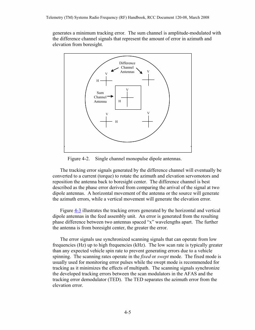
Telemetry (TM) Systems Radio Frequency (RF) Handbook, RCC Document 120-08, March 2008

TABLE OF CONTENTS

LIST OF FIGURES ............................................................................................................................................. iv

LIST OF TABLES................................................................................................................................................ v

PREFACE...........................................................................................................................................................vii

ACRONYMS AND INITIALISMS .................................................................................................................... ix

CHAPTER 1: OVERVIEW AND RADIO FREQUENCY (RF) BASICS ........................................1-1 1.1 Overview .........................................................................................................................1-1 1.2 Radio Frequency (RF) Basics ..........................................................................................1-2

CHAPTER 2: TRANSMIT SUBSYSTEM...........................................................................................2-1 2.1 Overview .........................................................................................................................2-1 2.2 System Configuration ......................................................................................................2-1 2.3 Telemetry Transmitters....................................................................................................2-5 2.4 Couplers and Cabling ....................................................................................................2-31 2.5 Transmit Antennas.........................................................................................................2-34

CHAPTER 3: RF CHANNEL...............................................................................................................3-1 3.1 Telemetry Bands..............................................................................................................3-1 3.2 Telemetry Channel Model (Multipath)............................................................................3-1 3.3 Other Channel Anomolies ...............................................................................................3-7

CHAPTER 4: RECEIVE SUBSYSTEMS............................................................................................4-1 4.1 Scope ...............................................................................................................................4-1 4.2 Introduction .....................................................................................................................4-1 4.3 Antenna Subsystem .........................................................................................................4-1 4.4 RF Subsystem ................................................................................................................4-12 4.5 Telemetry Receiver Subsystems....................................................................................4-14 4.6 System Sensitivity .........................................................................................................4-20 4.7 Signal Margin ................................................................................................................4-20 4.8 Link Analysis.................................................................................................................4-21 4.9 Dynamic Range .............................................................................................................4-30

CHAPTER 5: LESSONS LEARNED...................................................................................................5-1 5.1 Scope ...............................................................................................................................5-1 5.2 Testing of Permanently Installed RF Cables ...................................................................5-1 5.3 Radiation of Prelaunch Telemetry from Encapsulated Missiles ......................................5-1 5.4 Data Routing using Electronic Switching........................................................................5-2 5.5 Low Noise Amplifier (LNA) Characteristics ..................................................................5-3 5.6 Antenna Feed Dipole Design and Proper Phasing...........................................................5-3

APPENDIX A: FORM DD-1494 APPLICATION FOR EQUIPMENT

FREQUENCY ALLOCATION...................................................................................A-1

GLOSSARY

INDEX

iii


LIST OF FIGURES

Figure 1-1. Telemetry (TM) radio frequency (RF) system model.................................... 1-1 Figure 2-1. Configuration 1: Single transmitter - single antenna. ................................... 2-2 Figure 2-2. Configuration 2: Multiple transmitters - independent antennas. .................. 2-2 Figure 2-3. Configuration 3: Single transmitter - multiple antennas............................... 2-3 Figure 2-4. Configuration 4: Multiple transmitters - single antenna. .............................. 2-4 Figure 2-5. Configuration 5: Multiple transmitters - multiple antennas.......................... 2-4 Figure 2-6. Configuration 6: Complex telemetry transmit system. ................................. 2-5 Figure 2-7. BPSK block diagram...................................................................................... 2-7 Figure 2-8. QPSK block diagram. .................................................................................... 2-8 Figure 2-9. OQPSK block diagram. ................................................................................. 2-9 Figure 2-10. FQPSK-B wavelets. ..................................................................................... 2-10 Figure 2-11. FQPSK-B: I and Q signals.......................................................................... 2-10 Figure 2-12. FQPSK vector diagram. ............................................................................... 2-11 Figure 2-13. PCM/FM 1Mb 350KHz deviation. .............................................................. 2-15 Figure 2-14. PCM/FM 1Mb 250KHz deviation. .............................................................. 2-15 Figure 2-15. PCM/FM 1Mb 450KHz deviation. .............................................................. 2-16 Figure 2-16. Phase Modulation......................................................................................... 2-17 Figure 2-17. 10Mb/s NRZ PCM/FM. ............................................................................... 2-19 Figure 2-18. 10Mb/s SOQPSK-TG or FQPSK................................................................. 2-19 Figure 2-19. 10 Mb/s ARTM CPM. ................................................................................. 2-20 Figure 2-20. 5-Mb/s PCM eye pattern.............................................................................. 2-26 Figure 2-21. GPS filtering. ............................................................................................... 2-30 Figure 2-22. 4 Element Patch Array Azimuth (Az) Plane................................................ 2-36 Figure 2-23. 4 Element Patch Array Roll Plane. .............................................................. 2-37 Figure 2-24. Vehicle coordinate system. .......................................................................... 2-39 Figure 2-25. Antenna pattern for the pitch plane.............................................................. 2-40 Figure 2-26. Sample Antenna Radiation Distribution Table (ARDT). ............................ 2-42 Figure 3-1. Multipath........................................................................................................ 3-2 Figure 3-2. Tier 0 Channel Impairments. ......................................................................... 3-5 Figure 3-3. Tier 1 Channel Impairments. ......................................................................... 3-5 Figure 3-4. Receiver AGC................................................................................................ 3-6 Figure 4-1. Measurements used to calculate f /D ratio. .................................................... 4-4 Figure 4-2. Single channel monopulse dipole antennas. .................................................. 4-5 Figure 4-3. Tracking errors generated by dipole antennas. .............................................. 4-6 Figure 4-4. Typical sum channel and difference channel patterns (unscaled). ................ 4-7 Figure 4-5. Typical antenna pattern for conical scan feed assembly units. .................... 4-10 Figure 4-6. AM modulation error signal......................................................................... 4-12 Figure 4-7. Tracking error signals. ................................................................................. 4-16 Figure 4-8. Tracking error signals. ................................................................................. 4-17 Figure 4-9. Pictorial of parameters needed for measurement of transmitted gain.......... 4-23 Figure 4-10. Block diagram of RF units in the RF assembly. .......................................... 4-24 Figure 4-11. Block diagram of a sample RF subsystem................................................... 4-26 Figure 4-12. Frequency band interference........................................................................ 4-32

iv


LIST OF TABLES

Table 4-1. Comparison of Expected Noise Power ........................................................ 4-18 Table 4-2. Noise Contributed by Different IF BW Filters ............................................ 4-18 Table 4-3. Frequency Band Interference....................................................................... 4-32 Table 4-4. Sum and Difference ..................................................................................... 4-33

v


This page intentionally left blank.

vi


PREFACE

This document was prepared by the Radio Frequency (RF) Systems Committee of the Telemetry Group (TG), Range Commanders Council (RCC). The Committee objective is to have this handbook used as a useful tool for engineers and technicians working in the field of telemetry (TG) RF systems. This document is a “work in progress” and continues to be updated and improved over time. Therefore, the reader is encouraged to provide suggestions to identify additional areas of interest, areas needing more detail, and suggenstions on the content and the presentation. Please forward your suggestions or material you feel may be helpful in updating this document using the contact information below. The RCC gives special acknowledgement for production of this document to the RF Systems Committee. Please direct any questions to the committee’s point of contact or to the RCC Secretariat as shown below.

Point of Contact: Mr. Bob Selbrede RF Systems Committee Chairman Member Telemetry Group (TG) Air Force Flight Test Center 307 E. Popson Avenue Edwards Air Force Base (AFB), CA 93524-6630 Phone: DSN 527-1179 Com (661) 277-1179 Fax: DSN 527-6659 Com (661) 277-6659

Secretariat, Range Commanders Council ATTN: CSTE-DTC-WS-RCC (RF Systems Committee) 100 Headquarters Avenue White Sands Missile Range, New Mexico 88002-5110 Telephone: (505) 678-1107, DSN 258-1107

E-mail [email protected]

vii

mailto:[email protected]



viii


ACRONYMS AND INITIALISMS

AC/ac alternating current AFAS antenna feed assembly subsystem AGC automatic gain control AM amplitude modulation ARDT antenna radiation distribution table ARTM Advanced Range Telemetry Az/El azimuth/elevation BEP bit error probability BER bit error rate BiØ-L bi-phase level bps bits per second BPSK binary phase-shift keying BW bandwidth CCW counter clockwise CMRR common mode rejection ratio cos cosine CPFSK ontinuous phase frequency shift keying CPM continuous phase modulation cps cycles per second CSF conical scan feed CSFAU conical scan feed assembly unit CW continuous wave dB decibel dBc decibels referenced to the carrier (unmodulated) dBm decibels referenced to one milliwatt DC/dc direct current DSB double sideband ECC error correction coding EIRP effective isotropic radiated power EMC electromagnetic compatibility EMI electromagnetic interference ENR excess noise ratio ERP effective radiated power ESFAU electronically scanned feed assembly unit f/D focal length/aperture dimension FAU feed assembly unit FCC Federal Communications Commission FM frequency modulation FQPSK Feher’s quadrature phase-shift keying (patented) FQPSK-B A baseband filtered version of FQPSK FQPSK-JR A cross-correlated, constant envelope, spectrum shaped variant of FQPSK-B G/T gain/temperature; “figure of merit” GPS global positioning system

ix


Hz Hertz IAM incidental amplitude modulation ID identification IF intermediate frequency IFM incidental frequency modulation IM intermodulation IMD intermodulation distortion IP intercept point IRAC Interdepartmental Radio Advisory Committee IRIG Interrange Instrumentation Group ITU International Telecommunications Union K Kelvin kHz kilohertz LHCP left hand circular polarized LNA low noise amplifier LO local oscillator log logarithm LOS line of sight Mbps megabits per second MCEB Military Communications-Electronics Board MHz megahertz MIL STD military standard mps miles per second MSK minimum shift keying NPR noise power ratio NPRF noise power ratio floor NRZ-L non-return-to-zero-level NRZ-M non-return-to-zero-mark NRZ-S non-return-to-zero-space OQPSK offset quadrature phase-shift keying PAM pulse-amplitude modulation PCM pulse-code modulation PLD path length difference PLL phase-lock loop PM phase modulation p-p peak-to-peak PRN pseudo random noise PSAT saturated output power PSK phase shift keying PVC polyvinyl chloride QPSK quadrature phase-shift keying RF radio frequency RHCP right hand circular polarized rms root mean square RNRZ-L randomized non-return-to-zero-level RS Reed-Solomon

x


SCM single channel monopulse SFDR spurious free dynamic range SHF super high frequency sin sine SMA SubMiniature-version A (RF connector-type) SNR signal-to-noise ratio SOQPSK shaped offset quadrature phase shift keying SOQPSK-TG Waveform variant of SOQPSK; adopted by the Telemetry Group (TG) of the

Range Commanders Council in 2004 SSB single sideband SWR standing wave ratio TED tracking error demodulator THD total harmonic distortion TNC Threaded Neill-Concelman (RF connector-type) TSPI time-space position information TTL transistor-transistor logic UHF ultra high frequency Vdc volt direct current VHF very high frequency VSWR voltage standing wave ratio WARC-92 World Administrative Radio Conference – 1992

xi


xii



CHAPTER 1

OVERVIEW AND RADIO FREQUENCY (RF) BASICS

1.1 Overview

The Radio Frequency (RF) Systems Committee within the Telemetry Group (TG) of the Range Commanders Council (RCC) has prepared this document to assist in the development of improved RF telemetry transmitting and receiving systems in use on RCC member ranges. The TG expects that improved system design, operation, and maintenance will result from a better understanding of the factors that affect RF systems performance and, consequently, overall system effectiveness. Additional information can be found in RCC Document 119-06, Telemetry Applications Handbook.1

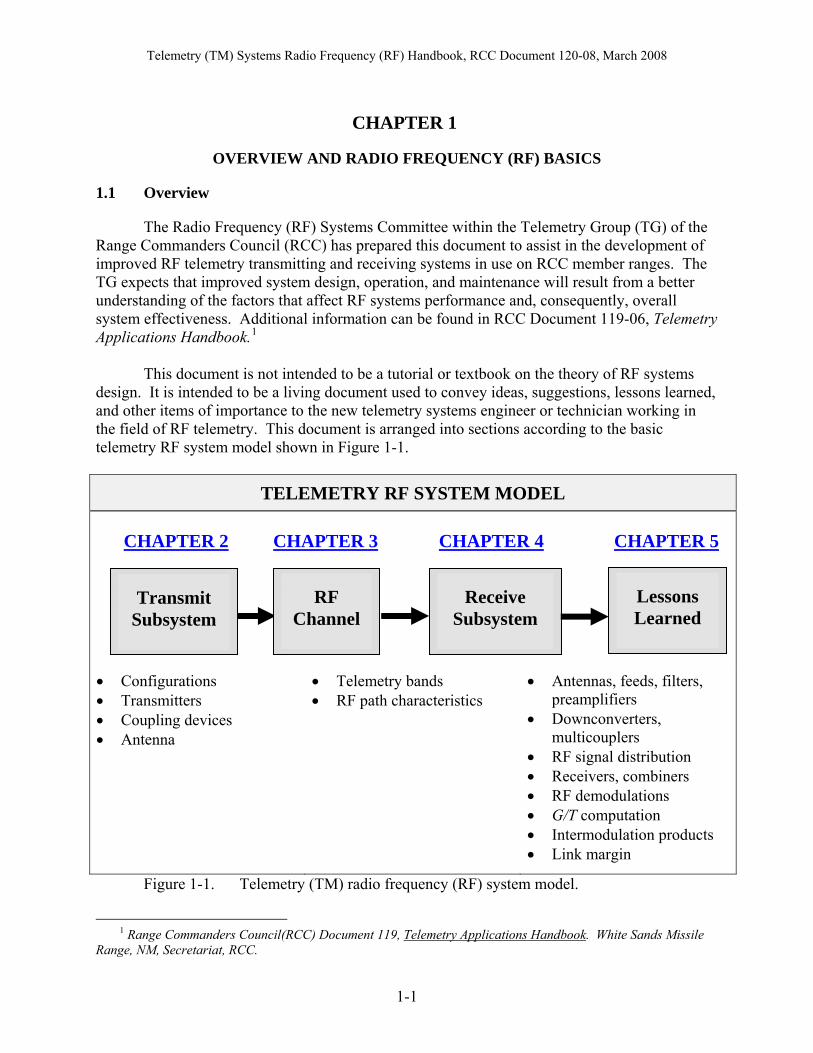
This document is not intended to be a tutorial or textbook on the theory of RF systems design. It is intended to be a living document used to convey ideas, suggestions, lessons learned, and other items of importance to the new telemetry systems engineer or technician working in the field of RF telemetry. This document is arranged into sections according to the basic telemetry RF system model shown in Figure 1-1.

TELEMETRY RF SYSTEM MODEL CHAPTER 2 CHAPTER 3 CHAPTER 4 CHAPTER 5

• Configurations • Transmitters • Coupling devices • Antenna

• Telemetry bands • RF path characteristics

• Antennas, feeds, filters, preamplifiers

• Downconverters, multicouplers

• RF signal distribution • Receivers, combiners • RF demodulations • G/T computation • Intermodulation products • Link margin

Figure 1-1. Telemetry (TM) radio frequency (RF) system model.

1 Range Commanders Council(RCC) Document 119, Telemetry Applications Handbook. White Sands Missile

Range, NM, Secretariat, RCC.

Receive Subsystem

RF Lessons Transmit Channel Subsystem Learned

1-1


1-2

1.2 Radio Frequency (RF) Basics

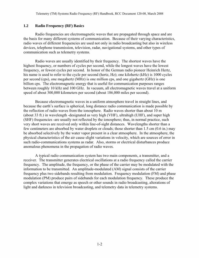
Radio frequencies are electromagnetic waves that are propagated through space and are the basis for many different systems of communication. Because of their varying characteristics, radio waves of different frequencies are used not only in radio broadcasting but also in wireless devices, telephone transmission, television, radar, navigational systems, and other types of communication such as telemetry systems. Radio waves are usually identified by their frequency. The shortest waves have the highest frequency, or numbers of cycles per second, while the longest waves have the lowest frequency, or fewest cycles per second. In honor of the German radio pioneer Heinrich Hertz, his name is used to refer to the cycle per second (hertz, Hz); one kilohertz (kHz) is 1000 cycles per second (cps), one megahertz (MHz) is one million cps, and one gigahertz (GHz) is one billion cps. The electromagnetic energy that is useful for communication purposes ranges between roughly 10 kHz and 100 GHz. In vacuum, all electromagnetic waves travel at a uniform speed of about 300,000 kilometers per second (about 186,000 miles per second). Because electromagnetic waves in a uniform atmosphere travel in straight lines, and because the earth’s surface is spherical, long distance radio communication is made possible by the reflection of radio waves from the ionosphere. Radio waves shorter than about 10 m (about 33 ft.) in wavelength -designated as very high (VHF), ultrahigh (UHF), and super high (SHF) frequencies -are usually not reflected by the ionosphere; thus, in normal practice, such very short waves are received only within line-of-sight distances. Wavelengths shorter than a few centimeters are absorbed by water droplets or clouds; those shorter than 1.5 cm (0.6 in.) may be absorbed selectively by the water vapor present in a clear atmosphere. In the atmosphere, the physical characteristics of the air cause slight variations in velocity, which are sources of error in such radio-communications systems as radar. Also, storms or electrical disturbances produce anomalous phenomena in the propagation of radio waves.

A typical radio communication system has two main components, a transmitter, and a receiver. The transmitter generates electrical oscillations at a radio frequency called the carrier frequency. The amplitude, the frequency, or the phase of the carrier may be modulated with the information to be transmitted. An amplitude-modulated (AM) signal consists of the carrier frequency plus two sidebands resulting from modulation. Frequency modulation (FM) and phase modulation (PM) produce pairs of sidebands for each modulation frequency. These produce the complex variations that emerge as speech or other sounds in radio broadcasting, alterations of light and darkness in television broadcasting, and telemetry data in telemetry systems.


CHAPTER 2

TRANSMIT SUBSYSTEM

2.1 Overview

This section of the handbook addresses the RF Transmit Subsystem and its associated components. It is intended to provide information and general guidelines for the proper design setup of airborne RF telemetry transmit systems. Telemetry transmitters, antenna systems, coupling devices, cabling, and related issues are discussed. 2.2 System Configurations

Telemetry transmit systems can be simple or very complex depending on the needs of the engineers and analysts who use the data. Figure 2-1 through Figure 2-6 depict various configurations of airborne RF telemetry systems currently used on Department of Defense (DoD) test ranges. A short discussion of these configurations is provided to help identify areas of concern that an RF telemetry systems engineer must be aware of when making design decisions. System configurations will ultimately be determined by any number of factors, including the number of independent telemetry data streams to be transmitted, the flight characteristics of the test vehicle, the space available for mounting transmitters and antennas, and the location of the ground station receiving the data. 2.2.1 Single Transmitter - Single Antenna. This configuration type (see Figure 2-1) represents the simplest form of an RF telemetry transmit system. In this configuration a single telemetry transmitter, operating on a specific assigned carrier frequency, is connected to a single telemetry antenna using some form of transmission line. To ensure that transmit-power losses are minimized, careful consideration should be given to the selection of high-quality coaxial cables and connectors, as well as the location of the transmitter with respect to the antenna. Every decibel (dB) of transmit-power loss directly affects the quality of received data. The location of antennas is important since proximity to other systems may result in interference from or to other communication systems on board the test vehicle. For example, Global Positioning System (GPS) receiver interference from L-band (1435-1525 MHz) transmitters is highly possible since its operating frequency is close to that of the telemetry system. Telemetry antennas should be located as far as possible from other antennas, especially those used for receiving signals on frequencies near the telemetry bands. Antennas that are used only for transmitting are not as critical.

2-1


Transmitter

Antenna

Transmission Line

Figure 2-1. Configuration 1: Single transmitter - single antenna.

2.2.2 Multiple Transmitters - Independent Antennas. When the need exists to transmit multiple telemetry data streams, a configuration of this type may be employed (Figure 2-2). Each transmitter requires an additional telemetry frequency assignment. This configuration utilizes separate antennas.

Transmitter #1

Antenna #1

Antenna #n

Transmitter #n

Transmission Line

Transmission Line

Figure 2-2. Configuration 2: Multiple transmitters - independent antennas.

2-2


2.2.3 Single Transmitter - Multiple Antennas. This configuration (Figure 2-3) is commonly found on aircraft when a single telemetry data stream is required. Aircraft antennas tend towards directionality, and aircraft surfaces are more likely to cause some signal blockage during maneuvers. Typically, one antenna is mounted on the top of the aircraft, and one is mounted on the bottom. The power split between antennas is usually 10 to 20 percent top and 80 to 90 percent bottom to reflect the fact that ground-based telemetry receiving stations are generally looking at the bottom of the aircraft. The top antenna comes into play when the aircraft is rolling or banking, causing the bottom antenna to be blocked by the fuselage or wings of the aircraft.

Ground stations can “see” both antennas at the same time. For this reason, 50/50 splits should be avoided in order to lessen the likelihood of having signal cancellation caused by both signals combining 180 degrees out of phase at the ground station. In order to ensure that the correct power split is achieved, the designer should measure the actual power at the antenna inputs to account for varying amounts of cable loss to the antennas. Adjustment in cable lengths may be necessary to ensure that the correct power split is achieved; however, the difference in cable lengths should be kept to a small fraction of the bit period as possible to maintain the proper phasing of the transmitted signal. Other test vehicles, such as missiles, may require only one antenna since it can be made to wrap around the body of the missile, providing coverage at most angles.

Antenna 1

Transmitter Antenna 2

Splitter

Figure 2-3. Configuration 3: Single transmitter - multiple antennas.

2.2.4 Multiple Transmitters - Single Antenna. A configuration which is more efficient in terms of using fewer antenna may be one in which an RF combiner allows multiple transmitters to drive one antenna. This configuration (Figure 2-4) is applicable when more than one transmitter is required and only one telemetry antenna is required (or allowed). Problems that could result from this configuration are the possible generation of mixing products and/or the transmission of spurious signals. If the transmitters mix with each other, due to RF from one transmitter getting into the output amplifier stage of the other transmitter, spurious transmissions will occur. This may be avoided by the addition of isolators between the outputs of the transmitters and the combiner. There is a 3 dB loss through the combiner for each transmitter signal, and the combiner needs to be able to dissipate the heat associated with this loss. An RF diplexer may be used (instead of the combiner) to combine multiple signals without this 3 dB loss if the

2-3


transmitter frequencies are known and fixed, and have sufficient frequency separation to allow for the proper filtering.

Antenna

Transmitter 1

Transmitter 2 Combiner

Figure 2-4. Configuration 4: Multiple transmitters - single antenna.

2.2.5 Multiple Transmitters - Multiple Antennas. This configuration (Figure 2-5) is a common one found on ranges today. Some test vehicles have two to three telemetry transmitters on them and generally one to two antennas. This is a hybrid of the other systems described above and the same precautions apply. If only two transmitters are required, the combiner and splitter may be replaced by a single four-port ring hybrid or 90-degree hybrid.

Antenna 1

Transmitter 1

Transmitter 2

Combiner

Antenna 2

Splitter

Figure 2-5. Configuration 5: Multiple transmitters - multiple antennas. 2.2.6 Complex Telemetry Transmit Systems. This configuration (Figure 2-6) illustrates how telemetry transmit systems can become quite complex in order to suit the needs of some test

2-4


programs. It is a composite of the other systems with the addition of several other special purpose components. In this illustration, directional couplers are used to tap off a low-level signal that could be used to monitor transmitter performance on a spectrum analyzer during ground tests. Combiners and splitters are used to send the outputs of multiple transmitters to upper and lower antennas while another transmitter is connected to upper and lower antennas of its own. This can be utilized for one or more authorized frequency bands. Coaxial switches are used to send transmitter outputs to dummy loads for testing purposes. Figure 2-6 is merely one illustration of the many possibilities for complex configurations.I

Xmtr 1

Xmtr 2

Xmtr 3

Switch

Coupler

Coupler

Xmtr Monitors

Coupler

Upper Ant 1

Upper Ant 2

Lower Ant 1

Lower Ant 2

Combiner

Dummy Load

Splitter

Splitter Switch

Dummy Load

Figure 2-6. Configuration 6: Complex telemetry transmit system. 2.3 Telemetry Transmitters

2.3.1 Introduction. Transmitters are used in telemetry systems for a variety of applications. They are utilized in stationary and mobile vehicle applications (including missiles and satellites) to relay data via digital or analog methods to a ground station, airborne station or relay site. Data can include discrete or analog performance data, Time-Space-Position-Information (TSPI), video, radar, GPS, onboard computer data, etc.

Telemetry transmitters are generally frequency-modulated (Tier 0). The transmitters generate a signal whose power output does not change with or without modulation. In some instances, phase-modulated transmitters are used, but this is less common. However, future high-bit-rate systems should make use of Feher’s quadrature phase-shift keying - Revision B (FQPSK-B) or other bandwidth-efficient modulation techniques (Tier 1 and Tier 2). This chapter is intended to provide an overview of transmitter characteristics that are important to consider when selecting or utilizing transmitters for telemetry applications in

2-5


accordance with the most recent IRIG-Standard 106.2 It is not a guide for the design of telemetry transmitters. 2.3.2 Types of Transmitters. Telemetry transmitters are available in various types designedspecific applications. Transmitters designed for rang

for e applications have typically been

equency-modulated (FM) transmitters with analog or digital modulation inputs. However, phase-m

frodulated (PM) transmitters are also in use.

a. FM Transmitters (Tier 0). An FM transmitter modulates data onto a continuous carrier. The data is conveyed in the deviation of the carrier frequency from no(1)

minal. Digital FM (Tier 0). Digital FM telemetry transmission is illustrated in some textbooks as a system in which two oscillators, one operating at the lower deviation limit and the other at the upper limit, are switched by the input. Suarrangement would lead to a phase discontinuity at the switching points. Rather, a digital modulator controls the frequency of a single local oscillator with a rapidly rising or falling square wave, making a frequency change without a phdiscontinuity. The implication is that, even with an instantaneous switching

ch an

ase

(2)

between the two frequencies, the bandwidth of the resulting signal, however measured, is lower than that which would result from the two-oscillator situation.Pulse Code Modulation (PCM) Systems. In binary PCM systems, the choice for a transmitted symbol is either a ONE or a ZERO; therefore, a dc term exists if theaverage number of ONES and ZEROS is not identical. A non-return-to-zero-level (NRZ-L) transmission with a balance of the two symbols would still need low-frequency response far lower than the bit rate, to accommodate the longest run ofONES or ZEROS that might be encountered in the data. This also places a limon how low the bit rate can be with respect to the low-frequency corner of acoupled system

it

n ac-. Different types of binary modulation have various effects on

transmitting spectra and, consequently, on transmitter and receiver system

b.

requirements.

Phase Modulation (PM) Systems. A PM transmitter modulates its data onto a continuous carrier. The data is conveyed in the deviation of the carrier phase from ainitial reference phase. A PM transmitter can be smaller and less complex than an FM transmitter because the modulator has no direct connection to the oscillator. Aphase m

n

odulator may well be a component of what might be called an FM system,

but the effect of modulation is to change only the phase, not the frequency, of the

carrier.

The instantaneous frequency of a signal whose phase is being advanced or retarded in proportion to the modulating voltage is indeed different from the frequency without modulation. A dc-voltage level fed into an FM modulator causes the output frequency to be different from the no-modulation condition. Any dc level applied to a phase-modulated transmitter produces only the carrier frequency itself. In this sense FM and PM transmitters are similar, since a received signal consisting of

2Range Commanders Council, Telemetry Group. RCC Standard 106 Telemetry Standard Part I and II. White Sands Missile Range, NM: Secretaria,).

2-6


a single sinusoid modulating a transmitter could appear the same coming from a Por an FM transmitter. More generally, an FM transmitte

M r fed a differentiated version

f an input signal fed directly to a PM transmitter could produce identical output

tran (1)

osignals, and a PM transmitter fed an integrated version of the signal fed to an FM

smitter could also produce the same output signals.

Binary Phase-Shift Keying System (BPSK). A BPSK transmitter (Figure 2-7) is one in which the modulating data produces a phase shift of the carrier atdefined states (0 and 180 degrees). BPSK also has a phase ambiguity problemNon-Return-to-Zero - Mark (NRZ-M), or Non-Return-to-Zero-Space (NRZ-S), issometimes used to solve this problem. Polarity ambiguity is caused bsuppression of the transmitted carrier so that the ground-station receiver must regenerate a reference carrier for demodulation. The generated reference carrier is obtained by squaring the entire signal in the receiver intermediate frequency (IF) bandwidth resulting in the demodulator reference either at 0 or 1

two pre- so

y

80 degrees with respect to the original carrier. The phase of the reference determines the polarity of the receiver PCM stream output. Since NRZ-M or NRZ-S code relies only on a bit change, and not the level, the polarity causes no ambiguity.

NRZ-L BPSK

cos ( ωOt )

Figure 2-7. BPSK block diagram.

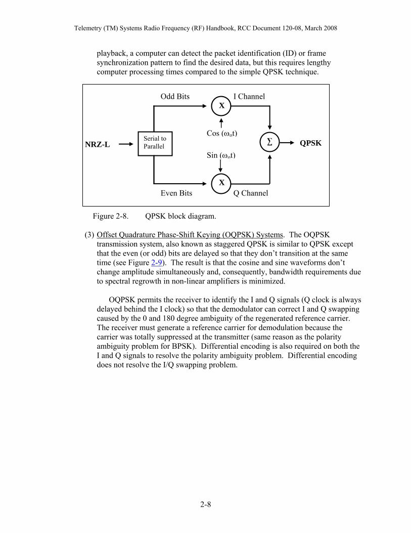
(2) Quadrature Phase-Shift Keying (QPSK) Systems. A QPSK transmitter is one in which the modulating data produces a phase shift of the carrier at four predefined states, for example, 0, 90, 180, and 270 degrees. The transmission system (Figure2-8) uses every other bit to modulate cosine and sine wave functions, athese are summed to produce the QPSK output. Phase ambiguity develops since the receiving system can only know the relative phase of the carrier and not thtrue phase. Coherent

nd

e detection is often used with QPSK systems because the

detection efficiency is typically better than non-coherent detection. In any event,

a at

PCM bit e

ring

the ambiguity problem must be solved by using methods such as differential encoding/decoding.

A special case of QPSK is asymmetric QPSK. In this case, differing datdiffering rates are sent on the I and Q channels. To detect this case, foursynchronizers with four frame synchronizers must be used to determine thcorrect I and Q signals as well as polarity for real-time processing. Du

2-7


playback, a computer can detect the packet identification (ID) or frame

F

(3)

synchronization pattern to find the desired data, but this requires lengthy computer processing times compared to the simple QPSK technique.

igure 2-8. QPSK block diagram.

Offset Quadrature Phase-Shift Keying (OQPSK) Systems. The OQPSK transmission system, also known as staggered QPSK is similar to QPSK except that the even (or odd) bits are delayed so that they don’t tran

sition at the same time (see Figure 2-9). The result is that the cosine and sine waveforms don’t

ays

ping

er (same reason as the polarity ambiguity problem for BPSK). Differential encoding is also required on both the I and Q signals to resolve the polarity ambiguity problem. Differential encoding does not resolve the I/Q swapping problem.

change amplitude simultaneously and, consequently, bandwidth requirements due to spectral regrowth in non-linear amplifiers is minimized.

OQPSK permits the receiver to identify the I and Q signals (Q clock is alwdelayed behind the I clock) so that the demodulator can correct I and Q swapcaused by the 0 and 180 degree ambiguity of the regenerated reference carrier. The receiver must generate a reference carrier for demodulation because the carrier was totally suppressed at the transmitt

Serial to Parallel

Even Bits Q Channel

Cos (ωot)

Sin (ωot)

Odd Bits I Channel

NRZ-L

X

X

∑ QPSK

2-8


Serial to Parallel

Delay Tb

Even Bits Q Channel

OQPSK Cos (ωot)

Sin (ωot)

Odd Bits I Channel

NRZ-L

X

X

∑

Figure 2-9. OQPSK block diagram.

(4) Feher’s Quadrature Phase-Shift Keying (FQPSK) System (Tier 1). The FQPSK3, 4 modulation is a variation of OQPSK where proprietary I and Q wavelet generation shaping is done. • Feher’s Quadrature Phase-Shift Keying (FQPSK-B) System (Tier 1).

Feher’s patented quadrature phase-shift keying (FQPSK-B: Rev A1) is one of the preferred modulation systems in IRIG-106 for bandwidth conservation. It is based on OQPSK with improvements to minimize amplitude variations, via the cross correlation of I and Q amplitudes, and further reduce bandwidth requirements especially in nonlinear amplifiers.

The typical implementation of FQPSK-B involves the application of data and a bit rate clock to the baseband processor of the quadrature modulator. The data are differentially encoded and converted to I and Q signals. The FQPSK-B I and Q channels are then cross-correlated and specialized wavelets are assembled which minimize the instantaneous variation of {I2(t) + Q2(t)}. The FQPSK-B baseband wavelets are illustrated in Figure-2-10. The appropriate wavelet is assembled based on the current and immediate past states of I and Q. Q is delayed by one-half symbol (one bit) with respect to I as shown in Figure 2-11.

3 K. Feher et al.: US Patents 4,567,602; 4,644,565; 5,491,457; and 5,784,402, post-patent improvements and other U.S. and international patents pending.

4Kato, Shuzo and Kamilo Feher, “XPSK: A New Cross-Correlated Phase Shift Keying Modulation Technique,” IEEE Trans. Comm., vol. COM-31, May 1983.

2-9


A common method of looking at I and Q modulation signals is called a vector diagram. One method of generating a vector diagram is to use an oscilloscope that has an XY mode. The vector diagram is generated by applying the I signal to the X input and the Q signal to the Y input. A sample vector diagram of FQPSK at the input terminals of an I-Q modulator is illustrated in Figure 2-12. Note that the vector diagram values are always within a few percent of being on a circle. The vector diagram of generalized filtered OQPSK would have more amplitude variations than FQPSK and the vector diagram of QPSK would go through the origin. Any amplitude variations may cause spectral spreading at the output of a non-linear amplifier.

0.4

2.6

0 3

I

Q

1

3

Ampl

itude

0 1

.707

-.707

1

-1

Figure 2-10. FQPSK-B wavelets. Figure 2-11. FQPSK-B: I and Q signals.

FQPSK-B (Revision A1) is the preferred modulation system for bandwidth conservation per IRIG Standard 106. Henceforth, any reference to FQPSK is a reference to FQPSK-B Revision A1.

• Feher’s Quadrature Phase-Shift Keying-JR (FQPSK-JR) System (Tier 1).

The FQPSK-JR is a cross-correlated, constant envelope, spectrum shaped variant of FQPSK-B. Its full definition can be found in IRIG-106 Chapter 2, paragraph 2.4.3.1.2 (IRIG-106 equals the online RCC Document 106, Part I-Telemetry Standards).

2-10


(5) Shaped Offset Quadrature Phase Shift Keying (SOQPSK) System (Tier 1). SOQPSK is a generic term for an infinite family of waveforms that shape (filter) the frequency pulse that precedes a frequency modulator. The filter for filtering the frequency pulse can assume an infinite number of shapes, thus a definition is required to insure interoperability. • Shaped Offset Quadrature Phase Shift Keying-TG (SOQPSK-TG) System

(Tier 1). SOQPSK-TG is the preferred method of SOQPSK for bandwidth and detection efficiency. The exact definition can be found in IRIG-106 Chapter 2, paragraph 2..4.3.2. It should be noted that FQPSK-B, FQPSK-JR, and SOQPSK-TG built to conform with IRIG-106 standards are interoperable.

(6) Continuous Phase Modulation (CPM) System. CPM is a generic classification of waveforms where the signal envelope is constant and phase varies in a continuous manner. • Continuous Phase Modulation-ARTM (ARTM CPM) System (Tier 2).

ARTM CPM is a specific version of CPM where the frequency pulse shape, modulation indices, and data mapping are specifically defined. Refer to IRIG-106 Chapter 2, paragraph 2.4.3.3.

-0.5

0

0.5

Q

-0.5 0 0.5

I

Figure 2-12. FQPSK vector diagram. 2.3.3 Characteristics and Parameters of Transmitters.

a. Modulation Characteristics (FM). An FM transmitter modulates data onto a continuous carrier. The data is conveyed in the deviation of the carrier frequency from nominal.

(1) Modulation Techniques.

2-11


• Analog FM. The analog transmitters typically utilized for telemetry

applications use the modulation input to control and change the frequency of a local oscillator. In a transmitter with an analog modulation input, the output frequency will linearly track the input signal’s instantaneous value.

• Digital FM. Current telemetry transmitters are not typically truly digital, but are a composite device with an analog transmitter with a digital modulation input. The circuitry in the modulation input converts the digital input signal to analog for transmission. The digital transmitter can be ac- or dc-coupled as in the case of the analog transmitter. The digital modulation input controls the frequency of a local oscillator and changes the frequency based on the input digital signal’s amplitude.

A digital transmitter has several advantages when compared to an analog transmitter. It is less sensitive to the modulation input signals’ wave shape and, therefore, the distance from the driver circuitry to the transmitter is less critical. Secondly, no premodulation filtering or deviation adjustment external to the transmitter is required; and, thirdly, linearity is not an issue with digital modulation. The one disadvantage of digital transmitters is that they are optimized for a single bit rate.

(2) Coupling. • AC Coupling. An ac-coupled transmitter eliminates the dc component of

the input waveform. In the case of randomized data, ac-coupling will have a minimal effect on the input data as long as the bit rate is equal to 4000 times the –3 dB frequency of the low-pass filter at the transmitter’s modulation input. However, if the input data is not randomized, or is otherwise asymmetrical, the frequencies of the transmitted ONES and ZEROS will not be equally spaced from the average frequency. In this case, the carrier will be offset resulting in a possible increase in errors at the receiving station.

• DC Coupling. A dc-coupled transmitter tracks the input signal linearly and any dc-offset component will be reflected in the carrier output. DC-coupled transmitters are typically harder to produce due to the requirement for a wider frequency response, starting at dc and increasing up to the bit rate frequency. Therefore, the best performance at the lowest cost is typically realized by utilizing an ac-coupled transmitter and randomized data.

(3) Modulation Frequency Response. The minimum and maximum frequency response required of a telemetry transmitter should be specified. Transmitters that do not meet the required frequency response for the data being transmitted adversely affect data quality due to amplitude reductions at high frequencies caused by transmitter-induced filtering. The frequency response can be determined from the change in peak deviation as a function of modulation frequency. If a carrier is modulated with a single sine or square wave, the relative amplitudes of the carrier components can be used to determine the peak deviation. The relative amplitudes of the carrier and observed sidebands can

2-12


also be used to calculate the peak deviation in situations where it is not possible to vary parameters to achieve a null.

(4) Modulation Sense. The modulation or deviation sense should be as specified in

the transmitter procurement document to prevent inversion of the digital data. The RCC standards specify that the carrier frequency shall increase when the voltage level on the modulation input increases and decrease when the modulation input voltage level decreases.

(5) Modulation Sensitivity. The correct modulation sensitivity, or carrier frequency shift relative to modulation input voltage, is critical for obtaining optimum data quality for a telemetry data link. The tolerance of the transmitter modulation sensitivity must be controlled to allow a given driver circuit to provide a consistent level of deviation of the transmitter (RF) output.

A transmitter has some sensitivity to input signals, which should be flat over the range of modulation frequencies that the transmitter is intended to operate. Typically, this is a small number of dB from the response at dc or some convenient mid-band frequency, often 1 kHz or 10 kHz. While the flatness of the response is tightly controlled for transmitters, the actual sensitivity may not be. Thus, transmitters from the same manufacturing lot may have a 2 dB (±10 percent) or more variation from one to another, unless the specification requires tighter tolerances. As a consequence, the actual deviation of the transmitter must be set for each telemetry set produced, and then checked and readjusted when the transmitter, modulator, or transmitter interface is replaced. This adjustment must be made as an RF measurement, not as a voltage measurement at the transmitter input. A transmitter’s input sensitivity may also be affected by temperature variations, which may be a concern if a wide operating temperature range is expected. The input sensitivity of a transmitter is expressed in several ways, which can result in significant confusion. Assuming that the output frequency is at center frequency when its input is shorted, deviation sensitivity can be expressed as the deviation resulting in a one-volt dc signal: ‘180 to 220 kHz per volt’. Then an ac signal of two volts peak-to-peak will cause a deviation in this example of 180 to 220 kHz, which is a true statement even if the transmitter doesn't have response down to dc. Assuming symmetrical modulation, there is a 2:1 difference between a peak voltage and a peak-to-peak voltage, so everything is still translatable into whatever system makes sense. If the transmitter deviation is specified as a deviation/Vrms value, the deviation specified is for a sine-wave input, and the actual deviation will vary for different input waveforms.

(6) Modulation Linearity. The modulation input voltage range required is dependent upon the specific telemetry system. The transmitter requirements should be specified such that the transmitter operates linearly for the specified modulation voltage range. Thus, the output carrier will linearly track the modulation input voltage for the required range.

2-13


• Modulation Overvoltage. Typically, a value is specified for an overvoltage

condition on the modulation input to prevent the transmitter from being damaged if a noise spike or other event causes the modulation input voltage to go out of the specified modulation voltage range. The transmitter will not operate linearly when this voltage is applied; however, it will resume proper operation after the modulation input voltage returns to its specified range for linear operation.

(7) Input Impedance. The amplitude accuracy of transmitted data can be adversely affected by a load mismatch at the transmitter modulation input. Improper input impedance matching can also cause unwanted filtering and oscillations at harmonic frequencies. A load mismatch can also overload and damage the driver circuitry feeding the transmitter modulation input. High frequency modulation passing through a multi-pin power connector can couple energy onto the power lines making it difficult to control unwanted emissions.

(8) Distortion. Harmonic distortion is caused by nonlinearities in the transmitter and results in output harmonics other than the fundamental frequency component.

(9) Common Mode Rejection. The common mode rejection ratio (CMRR) defines the susceptibility of the transmitter to common mode input signals or common mode noise. This property is important in applications that require a differential amplifier at the transmitter's modulation input.

(10) Reverse Conversion. A telemetry transmitter output circuit can act as a frequency converter by creating a spurious output when a reverse signal at frequency f2 applied to the transmitter output. Of primary concern is the conversion product at a frequency of (2 f1 − f2). This conversion product is symmetrically spaced on the opposite side of the transmitter frequency from the interfering signal ( f2 ). The conversion loss is nearly power-independent, but does vary somewhat with frequency offset (reference paragraph 1.2.4).

(11) Intermodulation Distortion (Two-Tone Intermodulation). Transmitters having nonlinear distortion can produce output frequencies equal to the sum and difference of multiples of the input frequencies.

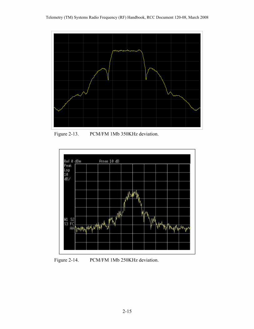
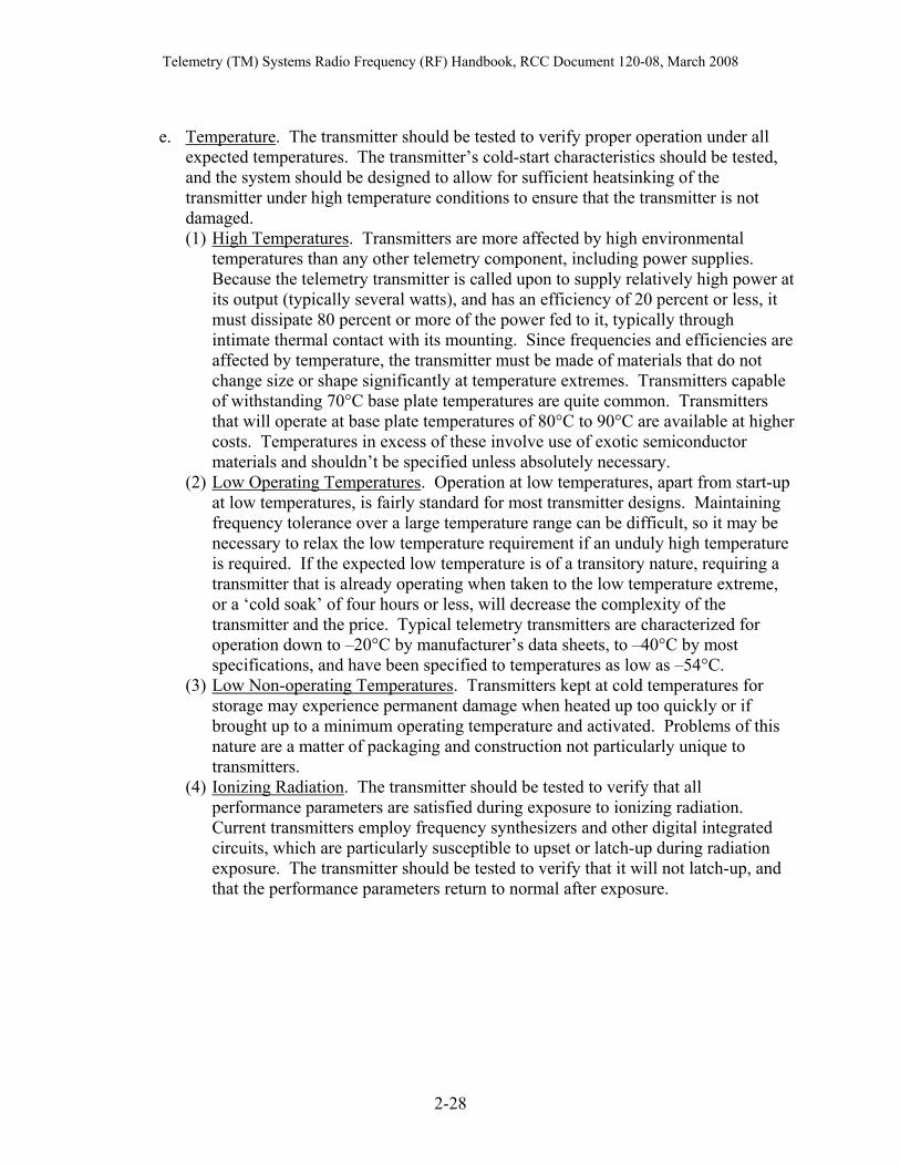
(12) Frequency Deviation. The proper frequency deviation for a given bit rate is necessary in order to obtain optimum bit error rate performance. For example, the modulation input driver circuitry for an Non-Return-To-Zero-Level (NRZ-L) data stream must be set to provide a peak deviation of 0.35 times the bit rate for optimum PCM data transmission (Figure 2-13). Under-deviation (much less than 0.35) (Figure 2-14) will result in poor data quality and over-deviation (much greater than 0.35) (Figure 2-15) may result in adjacent channel interference and degraded data quality in conditions with low signal to noise ratios.

2-14


Figure 2-13. PCM/FM 1Mb 350KHz deviation.


2-15



(13) Transition Threshold. The transition threshold required is dependent upon the logic device feeding the transmitter. It must be matched to the specified value in the transmitter procurement document in order to prevent the loss of, or unwanted addition of, bit transitions that would result in an increase in the bit error rate for the system. This only applies to digital transmitters.

(14) Premodulation Filters. The premodulation filter utilized must have sufficient attenuation characteristics to ensure that the transmitter’s RF spectrum will conform to the spectral mask requirements of IRIG Standard 106, Appendix A. The premodulation filter typically used for NRZ-L data is a six-pole Bessel filter with it’s -3 db cutoff set at 0.7 times the bit rate.

b. Modulation Characteristics (PM).

(1) Modulation Sense. The modulation sense of phase modulation systems is less standardized than that of PCM/FM systems, and it is important to specify the sense in transmitter-requirement documents.

(2) PM Deviation. FM deviation (Figure 2-16) is expressed in terms of the change between the center frequency and the instantaneous frequency at any point. With phase modulation, the center frequency never changes, and only the phase of the signal with regard to some reference changes. However, when the phase is in the act of changing, the instantaneous frequency is, in fact, different from the center frequency. Frequency and phase modulation are related by an integral (or a differential) such that an FM-like signal can be produced by integrating the modulation voltage and feeding it to a PM transmitter, and a PM-like signal can be produced by feeding the modulation voltage through a differentiator. For a single sinusoid input, therefore, it is impossible to determine if the transmitter is FM or PM.

2-16


Figure 2-16. Phase Modulation

PM is essentially a linear up-conversion while demodulation is a linear down-conversion. The input modulation spectrum display at baseband should provide the same spectrum display centered on the RF carrier frequency. The receiver intermediate frequency (IF) will also provide the same spectrum display as the carrier, only at the lower center frequency. Change of deviation only affects the carrier suppression. BPSK, QPSK, and MSK are also linear modulation with the spectrum display of the RF identical to the baseband spectrum display. FM is a non-linear modulation method that is apparent in the marked difference between the baseband and carrier spectrum display. Change of deviation causes great change in the carrier spectrum display. The transfer function of FM is parabolic so that the demodulator in the receiver must be parabolic as seen in the parabolic curve of noise or signal (baseband amplitude or demodulated output increases with frequency). Pre-emphasis, or additional baseband gain, is used as frequency increases to maintain the same signal-to-noise ratio for all the frequencies.

c. Modulation Characteristics (PSK) and Modulation Sense. The modulation sense of

FQPSK, which is a preferred method for bandwidth-efficient transmission, is defined in IRIG Standard 106.

2.3.4 How to Measure Power Relative to the Unmodulated Carrier Power Level. A common requirement is the need to measure a telemetry signal with respect to the unmodulated carrier level (units of dBc) but only the modulated signal may be available. To measure power with respect to the unmodulated carrier power, the unmodulated carrier power must be known. This

2-17


power level is the 0-dBc reference (commonly set to the top of the display). Since angle modulation (FM or PM) by its nature spreads the spectrum of a constant amount of power, a method to estimate the unmodulated carrier power is required if the modulation can not be turned off. For most practical angle modulated systems, the total carrier power at the spectrum analyzer input can be found by setting the spectrum analyzer's resolution and video bandwidths to their widest settings, setting the analyzer output to max hold, and allowing the analyzer to make several sweeps. The maximum value of this trace will be a good approximation of the unmodulated carrier level.

One can then set the spectrum analyzer to the IRIG 106 Chapter 2 conditions for measuring telemetry spectra (which in 2005 were resolution bandwidth = 30 kHz and video bandwidth = 300 Hz with max hold off). After measuring the signal spectrum, one can verify the 0 dBc level by finding the nominal peak level of the measured spectrum which should be about (X – 10logR) dBc.

Where X = -16 for PCM/FM with correct peak deviation, -12 for FQPSK and SOQPSK, -11 for ARTM CPM and R is bit rate (Mb/s). A more general approximation5 for the spectral energy near center frequency for randomized NRZ PCM/FM is

( ) ⎟⎟⎠

⎞⎜⎜⎝

⎛

Δ− 22

log10ffB bSA

π dBc

Where: BSA is spectrum analyzer resolution bandwidth in kHz fb is the bit rate in kb/s Δf is the peak deviation in kHz

Δf can be estimated1 using 2

spacingnullff b −=Δ

where null spacing is the frequency spacing between the closest spectral nulls on each side of the center frequency. Examples: If one measures the spectrum of a 10 Mb/s randomized NRZ PCM/FM signal with a peak deviation of 3.5 MHz one should get a maximum level of approximately –16-10log(10) = -26 dBc which matches quite well with the spectral plot shown in figure 1. Using the equation, one would get -10log(30*10000/(9.87*3500*3500) = -26.05 dBc or essentially the same value. If one measures the spectrum of a 10 Mb/s SOQPSK-TG signal the maximum level of the spectrum should be about –12 –10log(10) = -22 dBc (the tolerance should be about ± 1 dB). Figure 2-17, Figure 2-18, and Figure 2-19 show the measured spectra for 10 Mb/s signals with both wide spectrum analyzer settings (red traces, to find 0 dBc level) and IRIG 106 settings (blue traces). The actual 0 dBc values were found by removing the modulation. The approach presented here appears to work reasonably well for these modulation methods and bit rates up to at least 20 Mb/s. 5 Law, E. L., “RF Spectral Characteristics of Random NRZ PCM/FM and PSK Signals”, Proceedings of the 1991 International Telemetering Conference, pages 109-119, Las Vegas, NV.

2-18


-80

-60

-40

-20

0 P

ow

er

(dB

c)

-20 -10 0 10 20 Frequency (MHz)3M-MH 30k

10 Mb/s PCM/FM

Figure 2-17. 10Mb/s NRZ PCM/FM.

-80

-60

-40

-20

0

Pow

er (d

Bc)


10 Mb/s ARTM CPM

Figure 2-18. 10Mb/s SOQPSK-TG or FQPSK.

2-19


-80

-60

-40

-20

0

Pow

er (d

Bc)


10 Mb/s SOQPSK-TG or FQPSK

Figure 2-19. 10 Mb/s ARTM CPM. 2.3.5 Power Source Considerations.

a. Input Voltage. The input voltage range of typical telemetry transmitters is 24 to 32 Vdc. Telemetry transmitters for missile applications are typically powered by a battery, and for aircraft applications, by converted aircraft power. Therefore, in aircraft systems the noise immunity of the transmitters’ primary power input is more critical.

Transmitters typically use shunt regulators rather than dc-to-dc converters. Therefore, efficiency drops at higher operating voltage as the current drawn from the supply is relatively constant at any voltage at which the transmitter operates.

b. Input Current. The input current required by the transmitter is related to output power

and efficiency. The current source must be of low enough impedance to prevent variations in input voltage that could cause unwanted modulation within the transmitter.

c. Overvoltage/Undervoltage. The RF output and center frequency should meet

requirements at the limits of the primary power voltage range to ensure that the transmitter will operate as specified over the entire range of expected operating conditions. The transmitter should be designed so that the output stage shuts down in a low-voltage condition to prevent transmission outside the specified band of operation.

d. Reverse Polarity. The application of reverse voltage during testing and installation

can damage a telemetry transmitter if it is not properly protected. Circuitry to provide reverse voltage protection is typically built into telemetry transmitters.

2-20


e. Power Supply Ripple. The transmitter’s performance should be specified such that any expected ripple on power supply lines is rejected and doesn’t cause spurious emissions, unwanted frequency components, or modulation effects.

f. Tolerance. The transmitter power supply or battery must be of sufficient capacity to

provide the required voltage at full load under all environmental conditions. Typically, the transmitter will require a higher input current at high temperature.

g. Induced Power Supply Noise. Telemetry systems typically operate in an environment

where unwanted frequency components are present on the dc power leads to the telemetry transmitter. The transmitter must be designed such that induced power-supply noise does not cause unwanted frequency products within the transmitter. If the transmitter produces incidental AM and incidental FM components as a result of power-line noise, the received data quality will be adversely affected.

h. Power On/Off Characteristics. The turn-on and turn-off characteristics of the

transmitter must be such that no out-of-band emissions are generated during application or removal of primary power. In-band spurious emissions must be less than −25 dBm. This requirement is necessary to meet FCC regulations and to prevent interference with other users.

i. On/Off Switching (standby/operate). Transmitters may require on/off switching by

logic circuitry to prevent the transmitter from drawing excessive current from a system battery when not needed (to avoid overheating), or to prevent radiating when several transmitters have the same frequency. Turning the transmitter power on and off directly is often inconvenient because of the high currents and voltages involved, or because the transmitter would require time to warm up to power and get within frequency tolerance from a cold start.

Consequently, transmitters can be provided with a logic-controlled on/off lead that can be activated by discrete or monolithic logic or a combination of the two. The circuit is typically arranged so that grounding the control lead turns the transmitter on, and a logic ONE (or an open circuit) turns it off. With a load that approximates a TTL (transistor-transistor logic) unit load, or about 3 k ohms through the grounded lead. Especially if rapid start is required, the on/off circuit may control only the output stages, with the oscillator and modulator powered at all times power is applied, in which case a specification may limit the amount of power output produced when the transmitter is not turned on.

2.3.6 Grounding. The ground isolation at the telemetry transmitter should be specified to meet the requirements of the telemetry system design. The lack of a proper grounding scheme at the system level will typically cause noise that affects data quality and overall system performance.

a. Input Ground. The input ground of a transmitter may or may not be connected directly or indirectly to the case, modulator circuit ground, or RF ground, although in most situations it is common to all others. When a differential input is specified, the

2-21


ground associated with the input leads may or may not be common to the system case, and may be referred to a different voltage than case ground. The case ground will be common to the RF ground and probably the power ground. In most instances, the transmitter case is also common to the return of the input signal and control lines, if any.

2.3.7 Efficiency. The efficiency of a modern FM telemetry transmitter in the 1 to 20-watt operating range is on the order of 20 percent, up from the 8 to 10 percent found in designs from the 1960s. Efficiency is usually quoted at +24 Vdc, and typically decreases with increasing supply voltage. Since approximately 80 percent of the power consumed by a transmitter must be dissipated as heat, a 5-watt transmitter dissipates 25 watts of the 30 watts drawn from the external power. The 25 watts must be dissipated through a proper heatsink if the transmitter is operated for more than a few seconds. Transmitter overheating drastically shortens the life of the output stages. Efficiency considerations also limit the maximum output that can be obtained in a given system. The use of higher-power transmitters is generally precluded by restrictions of size, available power, and heat dissipation. 2.3.8 RF Output Characteristics.

a. Carrier Frequency. The center frequency and frequency stability are critical for avoiding interference with adjacent channels and for obtaining optimum data quality at the telemetry receiver. (1) Center Frequency. Typically, the unmodulated carrier output of an analog

transmitter is at the center frequency with no modulation input voltage, and it shifts up and down depending on the level of the modulation input voltage. In contrast, a digital transmitter, whose input is dc-coupled internally, has two possible output frequencies, f-lower and f-upper, and reaches frequencies between these two limits only when switching between states. Because the channel on which the transmitter operates is specified in terms of center frequency, the center frequency is specified as the average of f-lower and f-upper. This frequency would actually be the center frequency only when the transmitter was deviated with a square wave having exactly 50 percent duty cycle. For frequency management purposes, the band-edges with modulation (which are, in general, beyond those frequencies defined by f-lower and f-upper) are of far greater importance than some frequency in between.

(2) Carrier Noise. The unmodulated (and the modulated) carrier will have changes in amplitude, frequency, and phase regardless of which attribute is actually used for modulation. To the extent that the carrier exhibits the noise variations in the attribute used for modulation, the noise has a direct effect on signal-to-noise ratio on the demodulated signal. The effects of amplitude noise on a frequency-modulated transmitter, for example, are more subtle and exhibit themselves when the received-signal strength is low. The effects will vary with the type of receiver used and the nature of the modulation itself. For these reasons, the frequency, amplitude, and phase noise of any transmitter should be specified and measured.

2-22


b. Frequency Tolerance and Stability. The transmitter should meet specification requirements for each variation in operating environment. If the transmitter’s operation is adversely affected by specified temperature or power variations, the quality of received data may be unacceptable.

An FM transmitter will, when fed an open or short circuit instead of a modulated input, produce a signal that may be at or near the transmitter center frequency. In the case of tunable transmitters, the frequency should be the center or assigned frequency, although it may not be in the center of the frequency band when modulated. If the transmitter is ac-coupled (whether digital or analog), the frequency should be the center frequency, but in most cases it will not be exact. With dc-coupled analog transmitters, unless specified otherwise, the center frequency should be produced when the input voltage is 0 Vdc. With PM transmitters, the center frequency doesn’t change with modulation, but instantaneous frequency does, so measurement without modulation is required for accuracy.

c. Output Power . The telemetry system designer should complete a link analysis to

ensure that the specified transmitter power is sufficient for the expected maximum range of the telemetry system from the receiving site. However, the use of power in excess of the amount required should be limited as much as possible. Typically, output power will decrease at higher temperatures.

d. Output Impedance. The expected output load impedance of almost all telemetry

transmitters is 50 ohms and the output stage is tuned for such a load. That is not quite the same as saying that the output stage itself has an impedance of 50 ohms, but often an isolator is used between the output stage and the load, so that power reflected by the load will not be bounced back to the output stage.

e. Output Load Mismatch. Typically, antennas will not be perfectly matched to the

transmitter output impedance. This could be due to the antenna design or to external influences such as the plasma that develops around a vehicle during a reentry situation. In a mismatch condition, if inadequate output isolation exists, the transmitter may oscillate causing unwanted harmonics at its output, or it may fail to meet the minimum specified output power for a required mismatch condition. The transmitter may also shift in frequency if the output is not sufficiently isolated.

f. Isolation. Isolation of the transmitter output protects the transmitter from power that

is fed or reflected back into its output. Any extraneous load due to antennas, power splitters, and cables will not equal 50+j0 ohms, so a load voltage standing wave ratio (VSWR) greater than 1.0:1 will result. This VSWR will generally vary with frequency.

Transmitters without isolation will perform oddly when encountering reflected loads, either by greatly decreasing power output, or by generating spurious frequencies. The exact nature of this operation deviation will vary with the amplitude and phase of the reflected component, the temperature, and other extraneous factors

2-23


that cannot be easily traced. Hence, the transmitter must be specified to withstand a VSWR greater than the worst case expected at any phase angle. A typical requirement might be VSWRs as great as 3:1, which is half the power reflected. Some specifications go so far as to require near-infinite VSWRs due to open and short conditions on the transmitter output. Even an antenna that provides a particular maximum VSWR will cause a larger VSWR when loaded if it is in the proximity of other objects, such as a calibration stand or launch tube. This effect is exacerbated by a low-loss, high-efficiency antenna system. Therefore, a transmitter specification must take into account worst-case VSWRs.

g. Open and Short Circuit. The malfunction of an antenna component or operator error

during testing and installation may cause the transmitter to be subjected to an open or short condition. The relatively high cost of telemetry transmitters makes it desirable that the transmitter not be damaged should this condition occur.

Transmitters that have circulators or isolators at their outputs are normally capable of withstanding open- or short-circuited outputs. Assuming a perfect open or short, the entire transmitter output power is reflected back into the transmitter, to be dissipated at the dummy load in the circulator, which must be able to withstand the transmitter power for some length of time. If the dummy load is incapable of withstanding the transmitter output for long periods of time and/or at high temperatures or input power, permanent damage can occur even though the output is isolated. If the output of the transmitter is coupled to the output of another transmitter, the likelihood of permanent damage is further increased.

Not all transmitters contain isolators or circulators at their output, because of possible size restrictions and the fact that internal load resistors need a heatsink. Transmitters in which small size is a consideration often omit these output protection devices. Transmitters which are not equipped with isolators or circulators internally are less stable with regard to output impedance and load mismatch, and are consequently more subject to damage or erratic performance when the antenna is detuned or being affected by proximity to other forces.

h. Maximum Carrier Deviation. The bandwidth of the transmitter must be sufficient to

allow transmission of data at the maximum expected data rate. The optimum carrier deviation for NRZ-L PCM/FM is 0.35 times the bit rate, and the actual maximum carrier deviation for the transmitter must be greater than this value to ensure that data is not degraded by nonlinearities in the transmitter. The optimum carrier deviation varies depending on the modulation waveform selected.

i. Incidental Frequency Modulation (IFM). The IFM components created within the

transmitter may cause distortion that can degrade telemetry data and yield unacceptable quality data at the receiver. IFM is typically greater during vibration.

2-24


A spectrum display of adequate resolution will show that the observed center frequency is not a single spike but a tight bell-shaped curve. This phenomenon is partially due to the finite frequency characteristics of the filters used in the analyzer, but these can be minimized. It is also due to actual frequency modulation caused by thermal effects. A demodulated signal will show noise whose amplitude typically rises at 6 dB per octave due to white noise at the demodulator input, the same effect that would be noted for intentional phase modulation with a Gaussian white noise source. The rms deviation value for a typical FM telemetry transmitter in a 1 MHz bandwidth is around 1 to 2 kHz. The rms measure is used because of the statistical nature of the noise.

j. Incidental Amplitude Modulation (IAM). IAM occurring in a telemetry transmitter

will adversely affect the data quality at the output of a telemetry receiver through variations in transmitter power and the signal-to-noise ratio. IAM can also affect the accuracy of an antenna system that uses the telemetry signal for tracking. The use of a class C amplifier eliminates most of the IAM in telemetry transmitters.

k. Spurious Emissions. The occurrence of unwanted spurious and harmonic emissions

from a telemetry transmitter can adversely affect the system that is being monitored or systems outside the transmitter’s intended band of operation. It is, therefore, important that these emissions are controlled. GPS systems tend to be especially susceptible to telemetry systems operating in L-band.

The spurious emissions from the transmission system’s output should conform to the requirements set forth in IRIG-Standard 106. Spurious emissions can be generated within a transmitter. They can also result from improper termination or from multiple transmitter outputs terminating into a common antenna system, especially if the transmitter lacks sufficient output isolation.

l. DC Response and Linearity. Transmitters that are dc-coupled may be required for

some types of telemetry systems. Systems transmitting nonrandom PCM, pulse amplitude modulation (PAM), or some event marker data may require this type of transmitter.

m. AC Response and Linearity. The demodulated receiver output must accurately reflect

the amplitude of the input to the transmitter or data quality will be adversely affected. In PCM systems using an analog transmitter, poor ac-modulation linearity will increase the bit error rate of the received data. In PAM and FM/FM systems, poor ac-modulation linearity will have a greater adverse effect on the quality of received data.

n. Eye Pattern Response. The proper eye pattern response is a good indication that the

transmitter deviation, and the transmitter pre-modulation and receiver filtering are properly matched to provide acceptable bit error rate performance. A digital transmitter should have the proper eye pattern when modulated with a randomized NRZ-L (RNRZ-L) signal at the maximum specified bit rate. Figure 2-20 represents a good eye pattern for a 5 Mb/s PCM/FM signal.

2-25


Figure 2-20. 5-Mb/s PCM eye pattern.

o. Spectral Occupancy. The pre-modulation filter and peak deviation must be properly tuned to avoid interference with users on adjacent channels and transmission of RF frequency components outside the allocated frequency range of operation.

Bandwidth definitions are included in IRIG Standard 106. The bandwidth of the telemetry transmission system should be minimized by filtering and other methods, and conform to the spectral mask requirements included in IRIG-106. (1) Occupied Bandwidth. The occupied bandwidth (99-percent-power bandwidth) of

a telemetry transmitting system can be used to determine if the system complies with its RF spectral occupancy requirements.

(2) −25 dBm Bandwidth. The −25 dBm bandwidth of a telemetry transmitting system can be used to determine if the system complies with its RF spectral occupancy requirements. Spurious emissions must be less than −25 dBm to minimize interference levels to other systems.

p. Warm-up (Turn-on Time). The transmitter typically must meet specified

requirements during the warm-up period. Any spurious emissions emitted during the warm-up period shall be limited to −25 dBm. (1) Start-up. Because the transmitter contains an oscillator, its start-up response time

also affects signal output. Ideally, the oscillator should start and be up to full power instantaneously, but, in fact, the power output starts after some delay and rises more or less exponentially. The initial frequency is other than specified and may produce a signal that interferes with other users of the RF spectrum.

Typical transmitter specifications include a requirement that the transmitter center frequency be within the passband occupied by its spectrum after output power has exceeded –25 dBm, and also be within the required tolerances for the carrier within the specified number of seconds, typically 0.4 to 1.0. Power output is specified to be at or greater than the required minimum in two to ten seconds as

2-26


well. The IRIG-106 requirement should be considered the minimum acceptable performance.

(2) Cold start. Start-up or warm-up takes longer when the transmitter is in a colder

environment. Since oscillators are triggered by thermal noise, the possibility exists that if the transmitter encounters a colder temperature than that for which it is designed, it may not start up at all. Hence, testing of a transmitter whose warm-up time is critical is performed at the low-temperature limit. A dc-coupled receiver of known precision can be used to indicate the center frequency.

2.3.9 Environmental Considerations. Telemetry data are often most important when the system in which the transmitter is being utilized begins acting outside its expected performance environment due to a failure or anomaly. These are typically the times when the collection of telemetry data is critical. Environmental considerations are, therefore, extremely important factors. The transmitter must be capable of performing in more adverse conditions than the system in which it is operating. The following are some of the environmental factors requiring assessment:

a. Vibration. The transmitter should be tested to verify that all performance parameters are satisfied under the maximum expected vibration environment. Transmitters are particularly susceptible to increased incidental frequency modulation (IFM) during vibration.

b. Shock. The transmitter should be tested to verify proper operation after the maximum expected shock event and/or proper operation during the shock event if measurement of shock is part of the test. The transmitter is often not required to meet all performance parameters if high shock levels are anticipated due to pyrotechnic events. However, spurious emissions must be limited to −25 dBm at all times.

c. Acceleration. The transmitter should be tested to verify that all performance parameters are met during maximum expected acceleration environments.

d. Altitude/Pressure. The transmitter should be tested to ensure that its structure will survive and performance requirements will be met during maximum expected altitude and pressure environments. At high altitude, the transmitter/antenna should be tested to verify that corona, arcing, and other effects do not occur at the antenna causing degraded performance.

Operation of a transmitter at high altitudes presents certain problems not encountered at ambient pressures, including outgassing from foam potting materials, which can (if the pressure change occurs quickly enough) deform shapes associated with tuning and frequency determination. Transmitters used in telemetry applications are seldom hermetically sealed, so the air spaces on the inside of the transmitter eventually adjust to the external air pressure. Gasses at low pressures are more inclined to develop a plasma between two points of different potential, a mechanism similar to that found in a neon tube. The most likely points at which such an effect might occur are in the output stages. The greatest problem in testing transmitters at high equivalent altitudes is getting an altitude chamber with an adequate seal, especially if operating power for the transmitter is applied from the outside.

2-27


e. Temperature. The transmitter should be tested to verify proper operation under all

expected temperatures. The transmitter’s cold-start characteristics should be tested, and the system should be designed to allow for sufficient heatsinking of the transmitter under high temperature conditions to ensure that the transmitter is not damaged. (1) High Temperatures. Transmitters are more affected by high environmental

temperatures than any other telemetry component, including power supplies. Because the telemetry transmitter is called upon to supply relatively high power at its output (typically several watts), and has an efficiency of 20 percent or less, it must dissipate 80 percent or more of the power fed to it, typically through intimate thermal contact with its mounting. Since frequencies and efficiencies are affected by temperature, the transmitter must be made of materials that do not change size or shape significantly at temperature extremes. Transmitters capable of withstanding 70°C base plate temperatures are quite common. Transmitters that will operate at base plate temperatures of 80°C to 90°C are available at higher costs. Temperatures in excess of these involve use of exotic semiconductor materials and shouldn’t be specified unless absolutely necessary.

(2) Low Operating Temperatures. Operation at low temperatures, apart from start-up at low temperatures, is fairly standard for most transmitter designs. Maintaining frequency tolerance over a large temperature range can be difficult, so it may be necessary to relax the low temperature requirement if an unduly high temperature is required. If the expected low temperature is of a transitory nature, requiring a transmitter that is already operating when taken to the low temperature extreme, or a ‘cold soak’ of four hours or less, will decrease the complexity of the transmitter and the price. Typical telemetry transmitters are characterized for operation down to –20°C by manufacturer’s data sheets, to –40°C by most specifications, and have been specified to temperatures as low as –54°C.

(3) Low Non-operating Temperatures. Transmitters kept at cold temperatures for storage may experience permanent damage when heated up too quickly or if brought up to a minimum operating temperature and activated. Problems of this nature are a matter of packaging and construction not particularly unique to transmitters.

(4) Ionizing Radiation. The transmitter should be tested to verify that all performance parameters are satisfied during exposure to ionizing radiation. Current transmitters employ frequency synthesizers and other digital integrated circuits, which are particularly susceptible to upset or latch-up during radiation exposure. The transmitter should be tested to verify that it will not latch-up, and that the performance parameters return to normal after exposure.

2-28


2.3.10 Methods of Testing.

a. Bit Error Rate (BER) Testing. BER testing is a simple method used to verify proper transmitter operation. BER testing cannot be used as a substitute for the testing of individual performance parameters. RCC Document 118-06, Volume 1, Chapter 5, outlines BER methods.

b. Deviation Measurements. The transmitter’s deviation can be measured by several

methods also outlined in RCC-118, Volume 2, Chapter 5. The proper deviation is necessary to guarantee optimum system performance, spectral containment, and minimum BER.

c. Spectral Response. The output spectrum of the transmitter transmission system

should conform to the limits of spectral masks calculated according to the IRIG Standard 1066. This assures that the required minimum bandwidth is utilized and that adjacent channel interference with other users in the telemetry band will be minimized.

d. RMS Measurements. Because transmitter input sensitivities are sometimes specified

in terms of peak deviation per input volt rms, a temptation exists to set transmitter deviation by adjusting the rms value of the modulating signal such that the desired deviation is obtained. This acceptable for initial power-up and checks, but the actual deviation should be measured per the guidelines in RCC-118, Volume 2, Chapter 5.

2.3.11 GPS/Telemetry Compatibility. Several articles have been written and studies completed about interference problems between GPS and telemetry on aircraft/missiles since GPS systems became standard on these airborne platforms. The problem is always one sided since the telemetry signals are of a greater magnitude that the GPS received signals. Installing filters to remove the interference has become the desired practice, but this is not always possible or feasible with a production GPS receiver. Also the practice of moving the antennae as far as possible from one another has produced favorable results. This is not always possible because of the size of the test article or where space has been allocated for the antennae. It must be noted that if both antenna are utilizing the vehicles outer skin for a ground plane (common antenna mounting practice), antenna coupling is still present through the conductive skin and will produce some interference. Thus the only effective way to reduce interference is by placing filters between the transmitter/receiver and their associated antennae (Figure 2-21). Other studies6 have shown that interference can be minimized by utilizing a steered beam GPS antenna. Once again this may not be possible if the aircraft/missile is utilizing a production GPS system that cannot be modified. It should be noted that the majority of studies have focused on L Band telemetry interference, but that any transmitter may exhibit spurious signals in the GPS bands.

6 Range Commanders Council, Telemetry Group. Test Methods for Telemetry Systems and Subsystems,

Volume 2: White Sands Missile Range, NM: Secretariat, RCC Document 118.

2-29


Documentation has shown that S Band transmitters can also exhibit these characteristics, but in theory, any RF transmitter could produce a harmonic at these frequencies also. “Typically at least 90 dB of attenuation (100 dB preferred) of the main telemetry signal and at least 40 to 50 dB of attenuation of the telemetry transmitter’s noise at 1575.42 MHz is required. Telemetry transmitters that have spurious outputs close to 1575.4 MHz may require more than 50 dB of isolation at 1575.4 MHz. The typical specification for spurious signals at the output of a telemetry transmitter is –25 dBm, however, levels much lower than -25 dBm can cause problems if the frequency is close to the GPS frequencies. Problems are less likely to exist when S-band telemetry transmitters are used but problems can occur if the transmitter has spurs close to the GPS frequencies or if the telemetry transmitter saturates the GPS LNA. Many typical antenna configurations do not provide sufficient isolation. Therefore, both a good bandpass filter before the GPS LNA and possibly a bandstop or bandpass filter at the L-band telemetry transmitter output will be required for good GPS performance. Telemetry transmitters with lower output levels near GPS frequencies would reduce the probability of needing the bandstop filter.

Figure 2-21. GPS filtering. 2.3.12 Electromagnetic Interference/Electromagnetic Compatibility (EMI/EMC). The transmitter should be tested in accordance with system EMI/EMC requirements to verify that the transmitter and other system components don’t interfere with each other’s proper operation. 2.3.13 Telemetry Frequency Bands. At the writing of this document, telemetry systems are in the 1435-1525 ( L Band), 2200-2290 (lower S Band), and 2360-2395 (upper S Band) MHz portions of the frequency spectrum. The actual spectrum assignments are dependent on the range at which the telemetry system is to be used. Local frequency managers will coordinate actual frequency assignments.

2-30


Some transmitters are programmed to operate at more than one frequency or more than one band. The exact frequency (or frequency range) for the transmitter is factory-set and must be specified when ordering.

2.3.14 Form DD-1494. The application form DD-1494 is used to request a frequency allocation for telemetry systems and all other military radio frequency systems. Appendix A contains a sample (completed) DD-1494 and guidance on how to download blank forms.

a. Authorization to Acquire. Because the operation of a transmitter produces a signal that competes with other signals on the electromagnetic spectrum, authorization to purchase or use transmitters requires that certain types of paperwork be completed in advance. While this authorization must theoretically be obtained prior to purchase of a transmitter, in telemetry systems the procurement is usually allowed if the appropriate forms have been submitted, since the process often takes a up to a year to complete (form DD-1494).

b. Authorization to Radiate. Permission to radiate, even from the ground or inside a

building, requires coordination with the local frequency management group. This is necessary because there are many potential users and a limited number of channels. Without coordination, the probability of a clash is significant and the consequences serious.

2.3.15 Connectors. Transmitters typically have two or three connectors. The transmitter output is provided on a coaxial connector or on a short pigtail terminated in an RF connector. Typical connectors for this purpose are the SubMiniature Version A (SMA) type or the larger Threaded Neill-Concelman (TNC) type, although others can be used. The modulation input to the transmitter may be on the same connector used for power and control leads, or may be a separate multi-pin or coaxial connector. Connectors for power, modulation and frequency selection are more variable in type and size. Power to the transmitter, ON/OFF (standby/operate; key up/key down) control, and forward/reverse power indications (if supplied) are generally in the same connector, even if the modulation input is separate. Since connectors, even miniature ones, take up space, transmitters can also be supplied with connections made by ‘solder hooks’ fed through hermetic glass insulating beads. 2.4 Couplers and Cabling

Coupler and cabling components utilized in telemetry transmit systems can vary from one installation to another. This aspect of telemetry system design is often overlooked or underestimated by the novice system engineer. Proper selection of coupler and cabling materials can make or break an otherwise well-engineered system. Listed below are some of the more frequently used components found in the transmit subsystem along with typical uses and important characteristics to consider when purchasing and/or using them.

2.4.1 Coaxial Cable. Coaxial cable is the primary means by which telemetry transmitters, antennas, and other RF components are interconnected in virtually all RF telemetry subsystems.

2-31


Coaxial cable (coax) comes in hundreds of different types, each designed with a specific application in mind. Unless a special circumstance exists, almost all coax used in RF telemetry applications will be low-loss, 50 ohm impedance, coax. Most will meet Mil-C-17 requirements as well. The most important coax cable properties a telemetry systems engineer should consider are the impedance, signal attenuation (usually measured in dB per 100 feet at specific frequencies), power handling capability, shielding properties, velocity factor, bend radius, and insulation. When selecting coaxial cable for an application, the system designer will need to consider the impedance of the signal source and load, the frequency range over which the cable will be used, and the allowable amount of signal loss at the frequencies of interest. Then other factors will help guide your cable selection. In most cases, maximum power handling capability won’t be a key factor, but it should still be considered. If the user is concerned about EMI/EMC issues, selecting a cable with 100 percent shielding is essential. This will limit the amount of signal leakage from the cable to neighboring cables and also limit the susceptibility of your cable to outside sources of interference. Another consideration is minimum bend radius. This can be a factor when selecting a cable for use in tight spaces such as on aircraft or missiles. Exceeding the minimum bend radius will damage the cable and cause other factors such as impedance to be compromised.

On occasion, cable velocity factor will be of importance. Velocity factor is the ratio of the speed of signal propagation through the cable to signal propagation in a vacuum (the speed of light). Velocity factors around 66 percent are common with most PVC dielectric cables. Velocity factors in the 80-95 percent range are common in foam or air dielectric cables. The velocity factor will have to be known when trying to phase match cables together or build a coaxial cable delay line.

Coax insulation is important to consider when running coax in a vent or plenum or on an

aircraft. PVC-jacketed cables give off a toxic gas when heated. Teflon-jacketed cables are a better choice in high-temperature applications or on aircraft where fires are a possibility.

2.4.2 Connectors and Adapters. Proper selection of connectors and adapters is an essential step in system design. Whenever possible choose the right connector for the type of cable and type of mating requirements of the equipment involved. Adapters should be avoided, if possible. They tend to be lossy and they also have a tendency to fail at the most inopportune time. If they are critical to the system design, then use a high quality adapter designed for the impedance and frequency range required.

Connectors come in a wide range of styles. The specific application will determine the need for constant impedance connectors, high power connectors, threaded or bayonet connectors, weatherproof outdoor or indoor connectors, and the mating requirements of the equipment and cable being used. Precision connectors are also available for applications where very low losses are desirable.

2.4.3 Coaxial Switches. Coaxial switches are uniquely designed for switching RF circuits. They are constructed in a manner that preserves the constant impedance of the circuit, usually 50

2-32


ohms. Coax switches have very low insertion loss and high isolation between ports. This makes them ideal for low signal level or high level RF applications. Coax switches are the preferred type of switch for high-power applications. The maximum number of switch cycles will be higher if the coaxial switch is operated with the RF power turned off. Pin diode switches are much faster than coax switches, but they do not hold up well in high-power circuits where VSWRs exceed 1.5:1. 2.4.4 Terminations. Terminations are used when you want a device to “see” a proper load at its inputs or outputs. Most terminations used in the RF telemetry world are low-power 50 ohm loads. Terminations are used on the unused ports of directional couplers and on hybrid couplers. Terminations, also known as dummy loads, are also used on the outputs of transmitters during laboratory tests. The main considerations when specifying terminations are impedance and power dissipation. Terminations are usually purely resistive since a reactive termination would have impedance that would vary with frequency. Improperly terminated test equipment could yield erroneous results. 2.4.5 Attenuators. Attenuators are used to lower signal levels to be compatible with more sensitive devices. Attenuators are typically made to cover specific frequency bands and are generally 50-ohm devices. Attenuators come in fixed values ranging from several dB up to 60 or more dB. There are also attenuators of the continuously variable (linear) type or the step variety with discrete steps of 1 or 10 dB. 2.4.6 Directional Couplers. Directional couplers are used in several different ways. One common use is to sample RF signals that are passing through the coupler without disconnecting cables or breaking the RF path. Directional couplers can also be used in a reverse fashion to inject a signal into the primary RF path through the coupler. Directional couplers have an RF input, RF output, and one or two sample ports. The sample ports are coupled to the forward and reverse direction of signal flow through the coupler. They are used to tap signals for monitoring purposes or to inject signals for system testing. Selection of which port you use depends on the direction of signal flow desired. Unused sample ports are frequently terminated with dummy loads when not in use. The primary parameters to consider in the selection of directional couplers are the frequency range, through-path insertion loss, coupling loss, the amount of coupling at the sampled ports (values of 10-30 dB are common), and the port to port isolation. 2.4.7 Splitters and Combiners. An RF splitter and an RF combiner (not to be confused with a diversity combiner) use essentially the same process to either split or combine signals. Splitters are used to split an RF signal to multiple loads while maintaining the impedance match of the circuit. The split is usually 3 dB for a two-way splitter and 6 dB for a four-way splitter, etc. In addition to the signal loss from the split, there are insertion losses encountered as well. Conversely, combiners are used to add or combine signals together. The combining is generally in-phase combining of RF signals. These also exhibit an insertion loss.

2-33


2.4.8 Isolators and Circulators. An isolator is a device, frequently a ferrite device, which allows RF to flow through it freely in one direction while exhibiting a high degree of attenuation to RF flowing through in the opposite direction. Isolators are commonly used to prevent RF energy from feeding back into the output circuitry of transmitters and amplifiers. A circulator is a more complex form of isolator. A circulator allows RF energy to circulate through it in one direction only and attenuate signals that are traveling in the opposite direction. The important parameters to consider for isolators and circulators are insertion loss (in the intended direction) and isolation of RF traveling in the opposite direction. 2.4.9 Diplexers and Triplexers. These devices are complex networks effectively composed of splitters, combiners, and filters interconnected to achieve a high degree of isolation in a multi-band system such as an antenna feed assembly. Diplexers are dual-band devices. Triplexers are tri-band devices. These special devices are frequently used in antenna systems where the antenna is simultaneously receiving and transmitting RF signals. A high degree of isolation is required in this instance to keep the high-level RF signals from saturating the sensitive receive components connected to the same antenna. 2.4.10 Hybrid Couplers. A hybrid coupler is a specific type of coupler used to perform a special function, usually in an antenna system. The most common type of hybrid coupler used in telemetry applications is the quadrature or “90 degree” hybrid. The quadrature hybrid is used to combine two orthogonal signals, usually linear RF signals, (vertical and horizontal polarization) to create a circularly polarized signal from antenna feeds. 2.4.11 Filters. Filters used in telemetry systems come in many different types for many different applications. The most common types are the band-pass filter, low-pass filter, high-pass filter, and band-stop or “notch” filters. Of these, the most common types in the RF telemetry world are the band-pass and band-stop filters. Band-pass filters are used in telemetry antenna feed assemblies to limit the amount of out-of-band RF that enters the sensitive preamplifiers. High level RF signals, either in-band or out-of-band, will cause the preamplifiers to saturate and become non-linear. This will result in a huge increase in intermodulation distortion in the receive system. The band-stop or “notch” filter is used to eliminate a specific band of frequencies from a system. When a specific band of frequencies is expected to cause interference to your system, use of a notch filter to reduce the level of those signals may be advisable. Low-pass filters pass all frequencies below a certain cut-off frequency. They are found many times in the output stages of transmitters and amplifiers to limit the spurious and harmonic content of the transmitted spectrum. High-pass filters are used to pass all frequencies above a certain cut-off frequency. They can also be used to limit the amount of RF energy from strong transmitters that enter the front end of an RF telemetry receive system. 2.5 Transmit Antennas

The most common types of telemetry antennas utilized for aircraft and missile applications are the blade, slot, and several variations of conformal antennas. The type of test

2-34


vehicle, flight dynamics and/or the “available real estate” will dictate the type of antenna to be utilized. Most applications will utilize one of the following types of antennas. 2.5.1 Blade Antenna. Blades are commonly found on aircraft. Blade antennas are simple and relatively inexpensive compared to other antenna styles. Blades can be purchased for any of the telemetry bands and can also be purchased as multi-band antennas, i.e. lower and upper S-band in one antenna. Blade antennas have an omni-directional pattern in the azimuth plane and generally have more limited coverage in the elevation plane. Some designs try to fill in the elevation plane in an attempt to fill the void that typically exists on monopole antennas. The overhead portions of the antenna pattern tend to have many nulls in them. 2.5.2 Slot Antenna. This is a common form of antenna found on missiles, drones, and occasionally on aircraft. The antenna is a flat conformal antenna capable of being attached to the surface of the test vehicle. The antenna is sometimes made up of several sections that are fed through a power divider network of some kind in order to create the desired radiation pattern. Slot antennas are used when the aerodynamics of the test vehicle must be preserved, and when a desire to steer a beam in a particular direction is desired. 2.5.3 Conformal Antenna. This is a common form of antenna found on missiles, rockets, launch vehicle, bombs and artillery rounds. The antenna is built into the body of the test vehicle and often is indistinguishable from the body itself. The antenna is sometimes made up of several sections that are fed through a power divider network of some kind in order to create the desired radiation pattern. Wrap-around or micro-strip antennas are used when the aerodynamics of the test vehicle must be preserved and space and weight are prime considerations. Figure 2-22 and Figure 2-23 depict a typical pattern from these types of antennae.

2-35


Figure 2-22. 4 Element Patch Array Azimuth (Az) Plane.

2-36


Figure 2-23. 4 Element Patch Array Roll Plane.

2.5.4 Important Antenna Characteristics. The main electrical (radio frequency) parameters to consider in an antenna are listed below. In addition to these parameters there are other important mechanical, aerodynamic, and environmental parameters to consider when selecting an antenna.

a. Operating Frequency. Operating frequency, or “operating bandwidth,” is a critical antenna parameter. This is generally the frequency range over which the antenna will be expected to perform with regard to pattern, gain, impedance matching, etc. Bandwidth is either specified between some upper and lower frequency or as a percentage of center frequency. The operating bandwidth is usually the point where the impedance falls outside the range for a 1.5:1 or 2.0:1 VSWR.

b. Impedance. The impedance of the antenna must match the impedance of the

transmission line feeding it. In terms of RF, it is generally 50 ohms. If the antenna impedance doesn’t match the transmission line impedance there will be a mismatch (a

2-37


high VSWR) and reflections will occur. A significant portion of your RF signal will never be radiated by the antenna. Instead, it will be reflected back into the transmitter output, potentially causing your transmitter to fail or causing any number of other problems to occur such as spurious transmissions or EMI/EMC problems. Matching impedance levels will facilitate maximum power transfer.

c. Voltage Standing Wave Ratio (VSWR). As mentioned above, VSWR is a very

important parameter to consider and measure on any antenna system. A poorly matched antenna or transmission line will alter results and may, in fact, cause harm to the transmitter system and perhaps other systems via spurious transmitter outputs. An incorrectly installed antenna can result in a poor VSWR match even if the antenna itself is proper for your application. This is usually the result of improper grounding of the antenna to the ground plane of the test vehicle. A good quality VSWR meter will measure the match of the antenna system prior to transmitting RF into it.

d. Power Capability. This capability is the maximum amount of continuous or peak

power that the antenna can handle without causing damage to itself. For most telemetry applications, a maximum of 10 watts is adequate.

e. Connector Types. The type of RF connector on the antenna is another important item

to be aware of. For the most part, connectors at telemetry frequencies are SMA or TNC connectors. On occasion you may find a type N connector. The SMA or TNC connectors are preferred over other types of RF connectors because they are constant impedance, have low insertion loss, and they are small in size.

f. Antenna Pattern and Gain.

(1) Vehicle Coordinate System. The vehicle has its own coordinate system (roll, yaw, pitch) as shown in Figure 2-24. The roll axis is orthogonal to the roll plane. The pitch axis is orthogonal to the pitch plane. The yaw axis is orthogonal to the yaw plane. Angle theta (θ) is measured along the roll axis from the nose (0o) of the vehicle to the tail (180o). Phi (ϕ) is the measured angle along the yaw vector that starts at 0o and is measured in the counterclockwise direction around the vehicle to 358o. If the object “rolls,” it is described as a rotation about the roll vector. Left or right movements are described as movements about the yaw vector. Up and down movements are described as movements about the pitch vector. All three vectors are orthogonal to each other.

2-38


Roll Axis

Yaw Axis

Pitch Axis

Pitch planeRoll Plane

Yaw Plane

θ = 0°

θ =180°

ϕ = 0°θ = 90°

ϕ = 90°θ = 90°

ϕ = 180° θ = 90°

ϕ =270° θ = 90°

Figure 2-24. Vehicle coordinate system.7

(2) Antenna Pattern. Transmit antenna gain values (from the antenna pattern) vary due to deformities in the body (shape, wings, etc.) of the vehicle. A polar plot of the transmitting antenna plotted with respect to its location on the vehicle shows where maximum and minimum gain values occur for a particular “cut.” Figure 2-25 illustrates a polar plot of a vehicle for the pitch plane, a principal coordinate plane.

(3) Antenna Radiation Distribution Table (ARDT). An ARDT consists of the gain values along the sphere of the theta and phi plane. One polar plot set of values for a given theta with phi from 0o to 358o will constitute a row of values in an ARDT as illustrated in Figure 2-26. A complete set of antenna gain values measured every 2o for theta and rotated 360o on phi would yield 90 rows of gain values, or:

90 · 180 = 16,200 values

7 Range Commanders Council, Telemetry Group. Missile Antenna Pattern Coordinate System and Data

Formats. White Sands Missile Range, NM: Secretariat, RCC, August 1993 (IRIG Standard 253-93).

2-39


0

45

90

135

180

225

270

315 0

0

-10

-10

-20

-20

-30

-30

-40

-40-50

Tail

Top

Nose

Bottom

Figure 2-25. Antenna pattern for the pitch plane.

For example, the polar plot in Figure 2-25 yields 180 values for theta and phi from 0o to 360o. The values can be checked on the polar plot shown. The circular levels identify gain values below the highest value (reference value of 0 dBi) of the antenna. These polar plots are antenna patterns that identify deep nulls. The nulls may not be seen in other types of patterns such as gain values from an antenna radiation table if the increment value of theta and phi is too high. The major disadvantage of the polar plot is that the gain identifies only a particular theta and phi and cannot be programmed to evaluate the entire sphere that characterizes the vehicle.

The antenna radiation distribution table (ARDT) illustrated in Figure 2-26 overcomes the problem inherent in polar plots by digitizing the gain values as a function of theta and phi. The major problem with this type of antenna pattern data is that, if the incremental measurements are spaced far apart, nulls could be missed in the evaluation. Gain measurements are normally made in increments of 0.5, 2.0 or 5.0 degrees for theta and phi. The smaller the increment, the better the

2-40


evaluation. The disadvantage is that the smaller the increment, the higher the cost. Figure 2-26 illustrates this type of antenna pattern table for the polar plot shown in Figure 2-25. Phi (ϕ) is shown along the horizontal-axis starting at 0o up to 358o in increments of 2o. Theta (θ) is measured along the vertical axis from 0o to 180o, also in increments of 2o. Incremental values of 10o can be used but yield lower resolution values. The recommended increment is 2o. The table entries represent the gain, in decibels, below and above the reference level. In this example, the reference level is 0 dBi. The gain values are from Figure 2-25 for 0 to 90 degrees in phi at theta = 0o. If you study the polar plot in Figure 2-25 and look at the values entered in Figure 2-26, you can see that most of the low gain values are found at the nose and the tail of the vehicle. For small missiles, the ARDT is measured in a controlled environment such as an anechoic chamber. The missile is oriented such that the nose of the missile faces the transmitting source. The measurement-start-angle for phi and theta is 0o. The missile is rotated 360o about the center (roll) axis while theta is fixed at 0o. Antenna gain measurements are made at each predetermined increment. After the first set of measurements, theta is increased by the predetermined increment angle and phi-rotated. The process continues until the missile has been rotated 180o in the roll axis (theta). There are occasions when the missile (or object, such as an aircraft) is too large or awkward for this procedure.

g. Polarization. All antennas radiate electromagnetic energy, which by definition, is a composite wave consisting of an electric field (E-field) and a magnetic field (H-field). The polarization of an antenna generally refers to the orientation of its radiated E-field with respect to the earth. The most common forms of polarization are linear and circular. A less common form is elliptical.

Linear polarization can be further broken down to “horizontal” and “vertical” (the E-field propagates parallel or perpendicular to the earth’s surface). The designation of an antenna as vertically or horizontally polarized is most meaningful for stationary antennas whose orientation isn’t changing with respect to the earth. For aircraft and missiles, which are spinning or constantly changing orientation, these terms aren’t particularly meaningful. The important aspect would be that they are linearly polarized. Blade antennas, which are common on aircraft, are generally linearly polarized.

2-41


PHI

0 2 4 ●●●●●● 180 ●●●●●● 354 356 358 0 -33 -20 -10 ●●●● -20 ●●●● -11 -21 -32 2 -31 -18 -9 -19 -10 -19 -30 4 -29 -16 -9 -18 -9 -19 -29

88 -22 -13 -7 +1 -2 -10 -21 90 -20 -11 -4 +3 -3 -9 -20 92 -23 -14 -8 0 -3 -21 -22 T

HE

TA

174 -30 -17 -10 -20 -11 -21 -32 176 -32 -29 -11 -21 -12 -22 -33 178 -33 -20 -10 -20 -11 -21 -32

Figure 2-26. Sample Antenna Radiation Distribution Table (ARDT).

Circularly polarized antennas are ones in which the E-field rotates circularly as the signal propagates through the atmosphere. These antennas are either right-hand-circular-polarized (RHCP) or left-hand-circular-polarized (LHCP) as dictated by the direction of rotation of the E-field. Some antennas, such as the helix antenna, generate circularly polarized signals due to their mechanical (spiral) construction. Others generate a circularly polarized wave by combing horizontal and vertical linear elements through a 90-degree polarization hybrid.

h. Radiation Efficiency. The radiation efficiency of an antenna is a measure of how

much of the RF signal, applied to its input, is radiated rather than dissipated by some other means. Generally speaking, this can be directly related to the antenna’s input impedance. Most antennas are designed to have an input impedance of 50 Ω. This is primarily because most radio systems and coaxial cable transmission lines are also 50 Ω. When your signal source (transmitter) matches your transmission line and your

2-42


transmission line matches your antenna, maximum power transfer and minimum VSWR are achieved.

Antennas are tuned circuits. They exhibit a 50 Ω impedance at their resonant (design) frequency. At the resonant frequency, the input impedance is purely resistive and any reactive components are canceled out. When operated above or below their operating bandwidth, they begin to exhibit significant capacitive or inductive reactance properties. The input impedance of an antenna under these circumstances has a resistive and reactive component to it. Antenna radiation efficiency is highest when the reactive components are at a minimum, and the purely resistive components are at a maximum. This is due to the fact that the resistive portion of the antenna impedance is the only part capable of radiating energy. The reactive component will generally dissipate the energy as heat.

2-43


2-44



CHAPTER 3

RF CHANNEL

3.1 Telemetry Bands

There are specific frequency bands allocated for telemetry use in the United States. Listed below are the bands and notes regarding their use. Additional information regarding telemetry frequency bands and spectrum utilization can be found in IRIG Standard 106, Telemetry Standards. The following frequency bands are currently in use in the United States. Frequency allocations for telemetry and other services do change occasionally, so the user is advised to contact their local Frequency Management Office prior to planning any new system designs and/or tests to ensure compliance with current regulations.

a. L-band: 1435 – 1525 MHz b. Upper L-band: 1755 – 1850 MHz c. S-band: 2200 – 2290 MHz d. Upper S-band: 2360 – 2395 MHz

3.1.1 Lower L-Band. This band is commonly used for aircraft and other “manned” flight tests that require telemetry support. Users of this band are advised to pay close attention to the potential of L-band transmitters interfering with GPS receivers on board their test vehicles. Steps can be taken to ensure compatibility. This is also a common band used by targets and drones. 3.1.2 Upper L-Band. This band is occasionally used for telemetry, but not on a wide scale. It is generally used for video applications. It is not an official band allocated for telemetry use, but it can be considered when planning a new flight test program, if the local frequency management office approves it. 3.1.3 Lower S-Band. This band is commonly used for missile, spacecraft and other “unmanned” flight tests requiring telemetry support. 3.1.4 Upper S-Band. This band is slowly being reallocated for other non-DoD uses. There is currently only 30 MHz of the original 80 MHz remaining for aeronautical telemetry usage. This band has not been designated specifically for manned or unmanned use, so either application is acceptable. 3.2 Telemetry Channel Model (Multipath)

Multipath is an everyday occurrence at test Ranges that telemeter data from airborne test articles to ground stations. Multipath interference is a problem in most wireless communication systems and occurs when there are multiple paths between the transmitter and receiver causing signal fading and signal outages (Figure 3-1). With the direct line of sight being the exception, these other propagation paths are the result of reflections due to the physical environment and its geometry relationship with the transmitting and receiving locations. The amount in which these

3-1


reflection cause distortions is dependant upon the relative amplitude and phase of the reflected signals and the characteristics of the receiving antenna.

Aircraft, missile or UAV

Receiving Station

REFLECTING SURFACE

LINE OF SIGHT (LOS) SIGNAL S1(t)

WEAKER, DELAYED REPLICA S2(t)

Figure 3-1. Multipath.

Channel models are mathematical representations of how the physical environment affects the transmitted signal. Another way of saying it is that the model should represent how multipath will affect the received (and transmitted) signal. They are important for assessing modulation schemes, equalization strategies, and coding techniques for a given environment. Without these models, multipath mitigation simulation of these methods and others would have little value. Models are broken into two types, narrowband and wideband. Coherence bandwidth will be discussed when explaining these models, so a definition is required. Coherence bandwidth is a statistical measure of the range of frequencies in which the channel is considered “flat”, i.e. the channel passes the signals with equal gain and linear phase. Narrowband channel models are appropriate for situations where the signal bandwidth of the signal is much less than the coherence bandwidth of the multipath fading process. This means that the individual reflections due to terrain are not resolvable in the signal bandwidth. For example, such models are the Rayleigh and Rice channel models. Wideband channel models are used when the signal bandwidth is close to or exceeds the coherence bandwidth of the multipath fading process. For this case, individual reflections are resolvable in the signal bandwidth. This can be modeled as a tap delay line with time varying coefficients to account for the time variations in the multipath. Many channel sounding flights over Edwards AFB took place in both the LandS-Band telemetry bands in order to illuminate the telemetry spectrum and measure how the environment affected the transmitted signal. This information was delivered to the Telemetry Lab at Brigham Young University for analysis and to derive a model for the aeronautical telemetry channel. In most test cases, an airborne platform radiates the modulated carrier through an omni-directional antenna. It should be obvious that energy is transmitted in all directions with the receive station

3-2


being in one of these directions. It should also be obvious that multiple rays will be received at the receive antenna dispersed in time. When the data was analyzed, this was indeed found to be the case. The wideband channel model for aeronautical telemetry is composed of three propagation paths: a line of sight direct path and two specular reflection paths. An equation for the transfer function of the channel can be defined as:

Equation 3-1 – Wideband Channel Transfer Function

where δ(t) is the direct path modeled as a unit impulse function

L is the number of rays, 3 for the complete model Гk is the amplitude of the k-path τk is the delay of the k-path

The first reflection path is characterized by a relative amplitude of 70-96 percent of the direct line-of-sight path amplitude with a propagation delay of 10-80ns. This path is the result of reflections caused by ground terrain, mostly by the large lake bed present at the Range. The second path has a much lower amplitude and longer delay. The relative amplitude is approximately 2-8 percent of the direct line-of-sight path amplitude with the mean delay on the order of 155 ns with an RMS spread of 74 ns. This second reflection is dependant upon flight profile and terrain.

For most telemetry signals, the applicable model to use is the wideband model. The other choice is the narrowband model. Flight data from Edwards AFB, Patuxent River NAS, and White Sands Missile Range were analyzed and the following model is presented.

The received signal, y(t), when assuming a narrowband model, can be represented by:

Equation 3-2 – Narrowband Channel Received Signal

The line of sight component has so(t) as the transmitted signal with A amplitude. The specular reflection component has the transmitted signal with τsp average time delay with B amplitude and Δωsp Doppler shift. The diffuse multipath component consists of all other low level multipath reflections which gets modeled as a random component ξ(t), τavg average delay, and Δωdiff average Doppler shift.

3-3


If a narrowband model is assumed, per the coherence bandwidth criteria, the occupied bandwidth of the transmitted signal must be small. If this is the case, the transmitted signal is probably PCM/FM (or CPFSK). For PCM/FM, so(t) can be expressed as”

so(t)=exp{jπhbnt/Tb}

Equation 3-3 – PCM/FM Signal Definition

Where h is the modulation index, 0.7 for IRIG-106 recommended PCM/FM, bn is the information bit (+1 or -1), and Tb is the bit time.

After data analysis of the channel characteristics, it is noted that the channel is a function

of three parameters, relative Doppler shift Δω, and two quantities defined as:

Г=B2/A2 which is the specular to direct power ratio and κ= A2/2σd

2 which is the direct to diffuse power ratio

Equation 3-4 – Narrowband Channel Parameter Definition

For the test Ranges analyzed, the specular to direct power ratio, Г, varies from 0 to 1, the direct to diffuse power ratio, κ, varies from -48 dB to 25 dB with most values between 10 dB to 20 dB, and the relative Doppler shift, Δω, varies from 0Hz to 1.45Hz. Examples The equations given above were supplied in order to mathematically describe the telemetry channel and to explain the anomalies that are present in every day flight operations. To better understand the channel effects, lab experiments were conducted in order to represent what is typically visualized in telemetry receive stations and control room during flight test activities. Figure 3-2 and Figure 3-3 represent two of the three tiers of IRIG-106 waveforms with and without channel impairments. The three plots show:

a. The unimpaired waveform or “reference” in the plots b. A second ray incident on the receive site delayed by 50ns and attenuated by 1 dB from

the line of sight path. c. a second ray incident on the receive site delayed by 300ns and attenuated by 1 dB from

the line of sight path. These plots are intended to show what the spectrum may look like under multipath situations. During these times, the demodulator may interpret the waveform incorrectly leading to bit errors, or, for a very severe event, such as those depicted, loose synchronization entirely.

3-4


PCM/FM Multipath Effects

Reference50ns, 1dB300ns, 1dB

\

Figure 3-2. Tier 0 Channel Impairments.

Tier 1 Multipath Effects

Reference50ns, 1dB300ns, 1dB

Figure 3-3. Tier 1 Channel Impairments.

Figure 3-4 is shown to illustrate the variations of the receiver automatic gain control (AGC) through a known flight path. Though nulls in AGC can be attributed to antenna tracking error or poor antenna patterns on-board the aircraft, this particular AGC log shows only nulls caused by multipath events. Each null or dip in the AGC value can be attributed to multipath events. For the deeper nulls, the multipath event is such that it appears to be a flat fade at the ground station.

3-5


Received Signal Strength HistoryARTM flight 78, Cords Road, westerly

0

0.5

1

1.5

2

2.5

3

3.5

100 120 140 160 180 200 220 240 260 280 300

Elapsed Time - Seconds

RSS

- Vo

lts (1

0 dB

/Vol

t)

AGC1AGC4

Figure 3-4. Receiver AGC. 3.2.1 References. References for the above paragraphs are: a. Proakis, J. (2001), Digital Communications. b. Rappaport, T.S.(1996), Wireless Communications Principles and Practice, Prentice Hall,

McGraw Hill. c. Rice, M., Davis, A., Bettweiser, C., “A Wideband Channel Model for Aeronautical

Telemetry – Part 1: Geometric Considerations and Experimental Configuration”, Proceeding of the International Telemetry Conference, San Diego, CA, October 2002.

d. Rice, M., Davis, A., Bettweiser, C., “A Wideband Channel Model for Aeronautical Telemetry – Part 2: Modeling Results”, Proceeding of the International Telemetry Conference, San Diego, CA, October 2002.

e. Rice, M., Davis, A., Bettweiser, C., “A Wideband Model for Aeronautical Telemetry”, IEEE Transactions on Aerospace and Electronic Systems, vol. 40, issue 1, pp. 57-69, January 2004

f. Rice, M., Davis, A., “A Multipath Channel Model for Wideband Aeronautical Telemetry”, Proceedings of the IEEE Military Communications Conference, Anaheim, CA, October 2002

g. Rice M., Dye, R., Welling, K., "Narrowband Channel Model for Aeronautical Telemetry”, IEEE Transactions on Aerospace and Electronic Systems, vol. 36, no. 4, pp 1371-1376, October 2000.

h. Welling K., Rice, M., "A Narrow-Band Channel Model for Aeronautical Telemetry," in Proceedings of the International Telemetering Conference, San Diego, CA, October 1998.

3-6


3.3 Other Channel Anomolies

Telemetry RF path characteristics can vary significantly from one test range to another. In additiona to multipath, other RF path characteristics that may be encountered that could severly limit the quality of an RF link. Several significant examples of these are described below. These can be major obstacles requiring careful consideration in the test-planning portion of any mission. Steps can also be taken to reduce the effects of these phenomena when designing telemetry ground stations. 3.3.1 Shadowing. Shadowing is a physical blockage of the line of sight (LOS) RF path between the transmit antenna and ground station receive antenna. This is generally caused by obstruction or blockage by terrain or by fuselage and/or wings. When maneuvering aircraft or missiles fly behind hills or into valleys, or when aircraft taxi behind buildings, a physical blockage or attenuation of the RF path occurs. Since telemetry signal propagation is almost totally dependent on the LOS path, this blockage will result in a near total loss of signal at the receive site. The only way to combat this form of path anomaly is to augment your primary receive site with additional sites having different coverage areas.

When aircraft or missiles maneuver, their own surfaces (such as wing or tail sections) can block or attenuate the LOS path for brief periods of time. These dropouts in signal will generally be short in duration, but still unacceptable to most test programs. The most common way to combat this problem is by the installation of multiple, strategically located, telemetry antennas on the test vehicle as specified in Section 1. The transmitter outputs are then split between the antennas, increasing the likelihood that at least one antenna will always be in view of the ground station at any given time. There is, however, a down side to this approach. When multiple antennas are used in an array, the resulting radiation pattern may be completely different than expected. The RF energy from the individual antennas will combine, in and out of phase, creating peaks and nulls in the antenna pattern. This can be modeled and measured. Care should be taken to ensure that the resulting pattern is desirable for your specific application. 3.3.2 Plume Attenuation. Plume effects occur when telemetry receive antennas are pointed at the plume of a rocket or missile in order to receive telemetry data. Plume studies are done on every new missile or rocket, but the reports are typically classified. The distortion caused by the plume is heavily dependant upon the motor type. Solid propellant motors normally have more severe effects on the telemetry signal than liquid propellant motors. This is due to the quantity of the particles within the plume and their size. Through measurements, studies, and analysis, the telemetry signal fades have been characterized to occur randomly over a range of 500Hz to 25kHz with fade durations as small as 0.04ms but averaging 0.1ms. One mitigation technique is to not position the receive antenna where its look angle is looking though the plume. Side look telemetry receive antennas are typically deployed to mitigate the plume look angle problem. A second mitigation technique involves polarization diversity. In the past, the observation has been made that signal fades when received through right hand circular (RHC) polarized and left hand circular (LHC) polarized receive antennas are sometimes independent. There is of course a drawback to these two techniques though. How do you determine which antenna is receiving the best telemetry signal and how and when do you switch? One way to determine this is a combining technique that uses telemetry receivers AM detected IF signals and AGC voltages along with it’s own phase lock loop. Keep in mind that

3-7


3-8

for any combing technique to work, independent (diverse) sources of the telemetry signal are required. For mitigating plume effects, the diversity combiner circuitry must be able to correctly determine and select the best channel at a very high sampling rate in order to recognize independent channel dropouts of perhaps 0.04 milliseconds duration.

3.3.3 References: References for the above paragraphs are:

a. “Dynamic Requirements for Diversity Combiners”, Streich, Little, Picket, ITC Proceedings 1972.

b. “Test and Evaluation of the AM/AGC Combiner Unit”, Shibata, Federal Electric Corporation for Vandenberg AFB, 1978.

3.3.4 RF Blackout. This condition typically occurs during spacecraft or ballistic missile reentry into the earth’s atmosphere. During reentry, highly ionized gases surround the vehicle resulting in absorption of RF energy. As the ionized gasses dissipate, the vehicle’s RF energy can again propagate outside the bounds of the vehicle. RF blackout periods can last up to several minutes in duration. 3.3.5 Ducting. Ducting is a phenomenon in which an RF signal propagates along a path as if controlled by some form of guide or “duct.” This can cause problems in that the signal could possibly skip over its intended target since it is constrained by the duct. The most common example of this occurs when a signal is propagating through a non-homogeneous atmosphere where there are several distinctly different layers of atmospheric density. For example, this can occur when there is a layer of hot air rising up from a very hot ground in summer. Depending on the frequencies involved, the RF signal will have a tendency to bounce off the different density mediums, causing it to travel as if it where in a “duct.” 3.3.6 Radio Horizon. Radio waves at telemetry band frequencies generally travel a direct line-of-sight path unless affected by some other phenomena as described above. However, there is a slight bending of radio waves that can occur as the signal propagates through a medium (other than a vacuum) such as the earth’s atmosphere. The end result is a lengthening or extension of the radio horizon slightly beyond the optical horizon. The distance of the radio horizon will depend on a number of factors, but it is generally about 10 to15 percent farther than the optical horizon.


CHAPTER 4

RECEIVE SUBSYSTEMS

4.1 Scope

This section provides an overview of receiving system characteristics that are important for obtaining telemetry data from a radiating source. The emphasis is on the RF receiving system and subsystems. The information is intended as a guide to ensure that the receiving system performance is optimized to receive sufficient signal-to-noise (S/N) for a given bit rate. This overview will address subsystem operations, problems, and proven correction methods.

4.2 Introduction

A receiving system receives data via a transmitted modulated carrier. It demodulates the telemetry carrier, records, and/or relays the data. The received data must be of very high fidelity and as close as possible to a direct replica (error free) of the transmitted data. The transmitted carrier can be in a vehicle that is moving or stationary. A moving vehicle can present four possible challenges to obtaining quality data:

a. Vehicle and tracking system dynamics b. Receiving the signal through antenna nulls c. Data degradation due to plume effects on the transmitting source d. Multipath effects

Transmitted carrier from a stationary vehicle can be presented with effects from item b and/or item d above.

For testing procedures and methods applicable to any subsystem, refer to the RCC Document 118.8

4.3 Antenna Subsystem

Telemetry tracking systems typically use parabolic antennas/reflectors. The goal is for the reflector to intercept as much of the energy as possible in the “main lobe,” but some of the energy spills over the edges creating side lobe levels. Side lobes can be described as wasted or unwanted power levels that could actually interfere with automatic tracking.

The selection of a reflector is governed by the telemetry requirements, such as desired gain, side lobe performance, system dynamics, and cost. The antenna should also be of a size, as large as practical, to meet the mobile or fixed-site requirements.

8 See footnote #5, p. 1-27.

4-1


The major problem with reflector antennas is obtaining a good relationship between the

tracking feed and the reflector. When the feed is defocused along the axis of symmetry, the condition is known as a quadratic or “square-law” phase error. The parameters affected are antenna gain and the first side lobe amplitude levels. The phase errors can cause the nulls between the side lobes and the main beam to disappear. The main beam looks like a roll-off and the first side lobe amplitudes are no longer distinct. When the feed of a paraboloidal reflector is displaced from its focal point and off-axis, the main beam moves in opposite direction. This yields lower gain and higher side lobe levels. The end result is poor tracking performance.

4.3.1 Antenna-Feed Assembly Subsystem (AFAS).

a. Purpose. The purpose of the AFAS is twofold. The primary purpose is to receive the RF signal from the intercepted space wave that is within the designed RF bandwidth of the antenna elements. The second purpose is to produce error signals that generate the torque (current) to the azimuth and elevation drive motors that rotate the antenna enabling it to follow the source of the carrier frequency automatically if it is moving in space.

The AFAS unit should be located at the focal point of a typical parabolic reflector to maximize the received signal level while minimizing the tracking errors. The tracking errors at antenna boresight, or RF center, should indicate low (if any) amount of azimuth or elevation (Az/El) crosstalk. The first side lobes should be 16 to 22 dB down from the main lobe to enhance low-elevation, automatic tracking and to minimize interference. There are three basic types of tracking feed assembly subsystems. One is the single channel monopulse (SCM). The SCM is a diode-switching scanned feed designed to generate the tracking errors. The second one is a conical scan feed (CSF). As the name implies, a cone, which is derived from a nutation (or “wobble”) effect from a moving part (typically a horn antenna), is used to generate the tracking errors. The third type is an electronically scanned feed. It combines the best features of the SCM and CSF to generate the tracking errors. Application and cost considerations will govern the selection process.

b. f /D Ratio. Regardless of the type of feed used, a very important factor to consider is

the f /D ratio. This parameter is a function of the focal length and aperture dimension (Figure 4-1). The feed should be located at the focal point along the axis of symmetry. At this location, you optimize the antenna gain and have good side lobe performances. That is, the first side lobe peaks are optimized. They are located several dBs below the peak of the main beam. A peak amplitude of the first side lobes at 18 dB below the peak of the main beam is considered a good measure. The lower the peak of the first side lobes, the better the performance of the antenna.

4-2


The latest designs of feed assemblies have shown typical side lobe peak levels at 21 dB below the main lobe beam. Also, proper location of the feed assembly at the focal point will yield deep, sharp nulls between the first side lobes and the main lobe. Optimizing these parameters will also minimize the effects of multipath transmissions. A range user decides the size of antenna he needs. The antenna could be used to track satellites, aircraft, missiles, helicopters, etc. If the system will be used to track all of the above, the recommended optimization should be for tracking high dynamic vehicles, such as missiles. The determination of the f /D ratio now becomes more critical. This ratio represents the relationship between the tracking error modulation and the tracking error gradient. The tracking error modulation should be high enough to allow a linear error-tracking gradient for the RF band(s) in which the system will operate. Optimizing these parameters will decrease crosstalk between the azimuth and elevation tracking errors. Optimizing the tracking error gradient involves the curvature (depth) of the parabolic reflector.

Some equations in this section are presented in MSWord Equation Editor format. When downloading this document into a software program that does not contain Equation Editor, there may be some alterations in the equations. Please review those equations carefully.

From equation:

f = D2 /(16 • d) (Eq. 4.3-1)

where:

f = focal length D = diameter of the antenna d = depth of the antenna,

the focal point is a function of the depth and the diameter of the antenna. The depth is measured from the rear of the reflector to the front as shown in Figure 4-1. The f /D ratio will be a value greater than zero and less than 1.0.

0.0 < f /D < 1.0

The higher the f /D ratio, the sharper the tracking error modulation. An f /D ratio from 0.5 to 0.7 should yield tracking modulation with minimum crosstalk. Optimization of the f /D ratio can be seen on feed assembly units that use scanners for beam switching or conical scanning.

4-3


The secondary antenna patterns of the scanned beams, when plotted together, will show the main beam crossover point. If one the beam patterns has a higher gain level than the other, the overall antenna gain will decrease and the system will exhibit crosstalk within the linear tracking error gradient. All of the parameters must be optimized together, which is a difficult, but not impossible, task. Once optimized, the spars should be pinned to the reflector and the feed assembly cage to allow feed removal and reassembly at the same focal point. This will also keep the feed from becoming skewed or defocused.

f D

Axis of Symmetry

d

Figure 4-1. Measurements used to calculate f /D ratio.

c. Single Channel Monopulse (SCM). This type of tracking feed assembly consists of a sum channel (Σ) and a difference channel (Δ). The sum channel is also known as the data channel for receiving the carrier frequency (modulated or unmodulated). The difference channel (Δ) generates signals (known as tracking error signals) for automatic tracking. Dipole antennas are typically used and tuned to the frequency band(s) assigned for telemetry. If the frequency band is very wide, such that it covers more than one band, as from 1400 MHz to 2400 MHz, it becomes difficult to tune the dipole antennas. The end result could be unwanted crosstalk, lower gain, a higher axial ratio, and possibly a decrease in the tracking error gradient linearity.

The sum channel dipole antennas are usually in a crossed dipole configuration as illustrated in Figure 4-2. The crossed dipoles are orthogonal to each other and referenced as vertical and horizontal. The difference channel dipole antennas are also in a crossed dipole configuration, and situated around the sum channel dipole antennas with some isolation for minimizing antenna crosstalk. The sum channel receives the maximum signal level when it is properly boresighted since it is located at the focal point. This position corresponds to where the difference channel

4-4


generates a minimum tracking error. The sum channel is amplitude-modulated with the difference channel signals that represent the amount of error in azimuth and elevation from boresight.

V H

Sum Channel Antenna

Difference Channel Antennas V

V

V

H

V

H

Figure 4-2. Single channel monopulse dipole antennas.

The tracking error signals generated by the difference channel will eventually be converted to a current (torque) to rotate the azimuth and elevation servomotors and reposition the antenna back to boresight center. The difference channel is best described as the phase error derived from comparing the arrival of the signal at two dipole antennas. A horizontal movement of the antenna or the source will generate the azimuth errors, while a vertical movement will generate the elevation error.

Figure 4-3 illustrates the tracking errors generated by the horizontal and vertical dipole antennas in the feed assembly unit. An error is generated from the resulting phase difference between two antennas spaced “x” wavelengths apart. The further the antenna is from boresight center, the greater the error. The error signals use synchronized scanning signals that can operate from low frequencies (Hz) up to high frequencies (kHz). The low scan rate is typically greater than any expected vehicle spin rate to prevent generating errors due to a vehicle spinning. The scanning rates operate in the fixed or swept mode. The fixed mode is usually used for monitoring error pulses while the swept mode is recommended for tracking as it minimizes the effects of multipath. The scanning signals synchronize the developed tracking errors between the scan modulators in the AFAS and the tracking error demodulator (TED). The TED separates the azimuth error from the elevation error.

4-5


NOTE:

The farther the Az/El error pulses are from the reference point, the greater the error. Note that the 0-degree phase equals the “mirror image” at 180 degrees.

Volts 0 Deg Phase 180 Deg Phase Az El El 0 Az Volts

Tracking errorpulses generated by the PLD MISSILE

R R2 1

PLD

Feed Ant H - dipole

Feed Ant H-dipole

BASELINE = BL

PLD: Path length difference; generates the error

that represents how much server oh correction is needed to rotate the antenna back to boresight center; stated in multiples of wavelengths were fractions of a wavelength and equal to r1 – r2.

c/ f: Wavelength.

R1, R2: Range between missile and antennas at any given time.

BL: Baseline distance between antennas (approximately six inches).

Figure 4-3. Tracking errors generated by dipole antennas.

4-6


(1) Antenna Patterns for SCM. The secondary antenna pattern for the sum channel follows the sin x/x waveform. Figure 4-4 illustrates the typical antenna patterns for sum channel (solid line) and difference channel (broken line). Deep nulls should be evident between the main lobe and succeeding side lobes if the AFAS is at the focal point. Succeeding side lobe amplitudes should be lower than their preceding side-lobe level. The first side lobes should be at least 16 dB down from the main lobe.

The difference pattern is just the opposite of the sum channel pattern. A deep null in the difference pattern should occur everywhere that the sum channel pattern indicates a maximum signal. Care should be taken to prevent “side-lobe shoulders” where there is no deep null between side lobes.

Figure 4-4. Typical sum channel and difference channel patterns (unscaled).

Figure 4-4 shows the pattern limits to be from –18.0o to +18.0o for the purpose of examining the main lobe, and at least the first two side-lobe levels. Antenna patterns can extend from –360o to +360o where back lobes would be evident, but the resolution is not very good.

(2) Skew Condition for SCM. A skew condition of the feed assembly unit (FAU) is

an example of a phasing problem and may not be obvious to the naked eye. A skew condition can be assessed through an antenna pattern measurement using a boresight source. Knowing the exact azimuth and elevation angle between the receive system and the boresight source can help the assessment.

A skew condition can be evaluated by tracking an RF source (using the auto-track mode) radiating from a known, surveyed point, and monitoring the receiver AM output or the input to the TED. The typical four tracking error pulses (Az/El)

4-7


for 0o and 180o should be almost a straight line.9 The auto-track azimuth and elevation angles between the tracking system and the boresight source should be within 5 percent (static error) of the position angles to the source for maximum signal. If the antenna movement about the true position angles is greater than the gradient linearity limit, or if the tracking errors indicate a wide dispersion while in the auto-track mode, the system is a good candidate for feed re-alignment. It is important to confirm that the antenna spars are not loose and causing the FAU to skew. Also, the transmitting source should be located at a distance for far-field analysis, which is determined by the diameter of the receiving reflector.

(3) Error Crosstalk for SCM. Error crosstalk in an “elevation over azimuth” system

is a very serious problem that can prevent auto-tracking. Crosstalk occurs when you generate the tracking error in one axis only and the other axis indicates an error that can cause movement. A common symptom is a spiraling movement of the antenna due to the attempts to correct the generated tracking error from an error that is not real. There should not be a crosstalk error indication on the axis that has not been rotated. The tracking error gradient limit should be free of crosstalk. This limit is referenced at the −3 dB beam width of the antenna. Error crosstalk should be monitored during acceptance testing. Areas of assessment should include the following: • The parabolic reflector should have an f /D ratio set to optimize the

tracking performance by increasing the tracking error modulation. The f /D ratio is the ratio of the focal length divided by the diameter (aperture) of the antenna.

• The error crosstalk condition of the system should be evaluated using linear polarization and circular polarization transmission sources.

• Error crosstalk conditions should also include verification that multipath is not a source or a result of crosstalk.

A valid check of these conditions should be made if you are not convinced that the feed assembly components are individually or collectively in working order.

d. Conical Scan Feed Assembly Unit (CSFAU). This type of tracking feed is based on

the principle of a rotating horn coupled to a motor. Typically, two dipole antennas are orthogonal to each other and directly behind the horn to receive the space energy. The dipole antennas are tuned to the frequency band of interest and can be subject to crosstalk or non-linear tracking error gradient similar to an SCM feed. The rotation is known as “nutation” or a “wobbling” motion. Most feed assembly units of this type use a fixed motor speed (usually fixed at 30 Hz) to rotate the horn.

The latest feed units can have variable, rotating speeds to offset any missile rotation that can interfere with the motor rotation speed that affects the generation of the tracking errors. The horn is offset to cause the beam of the secondary pattern to

9 See footnote No. 5 on p. 1-27.

4-8


be reflected off-axis. The rotating horn amplitude modulates the incoming RF energy. The resulting amplitude and phase of the modulation is indicative of the magnitude of the error that corresponds to the amount of angular offset from center.

The error information is processed by the tracking receiver AM circuit and separated by a tracking error demodulator into the azimuth and elevation position errors. This type of feed assembly has an optical commutator that provides two quadrature square waves for reference. The reference signals are synchronized with the receiver AM output to derive the azimuth and elevation tracking error signals. The error signals are used to command the antenna to track the radiating source.

(1) Antenna Patterns for CSFAU. Two different types of antenna pattern

measurements should be conducted. The first one is with the scanners turned off. This pattern checks for symmetry, side-lobe levels, and beam width. The second one involves two sets of measurements with the scanners on. For the first set of patterns, the antenna should be rotated from right-to-left. For the second set of patterns the antenna should be rotated from left-to-right for the same start/stop angles.

With the scanners on, the two traces will look similar to those illustrated in Figure 4-5. Notice that on one trace, one side lobe is higher than the other. On the second measurement, the opposite side lobe is higher. The crossover at peak signal should be at the same point. One side lobe being higher is a condition called “coma lobe.” The opposite side lobe is suppressed. This is due to the nutation movement. The nutation causes the focal point to be displaced off-center as it scans around the main focal point. The crossover point of both patterns should be at the same point. Any displacement of the crossover point indicates decreased gain and error modulation that is not very linear.

4-9


Clear, Sharp Nulls

Max Signal

First side lobe -20 dB

Coma lobe

Suppressed lobe

-------------- Difference channel antenna pattern

Sum channel antenna pattern

Figure 4-5. Typical antenna pattern for conical scan feed assembly units.

(2) Skew Conditions for CSFAU. A skew condition of the conical scan feed assembly unit (CSFAU) is an example of phasing problems similar to the single channel monopulse feed. The skew condition may not be obvious to the naked eye. A skew condition can be assessed by conducting an antenna-pattern measurement using a boresight source. The antenna pattern should be conducted with the scanners turned off to assess symmetry. This ensures that the focal point is centered about the crossed dipoles.

The auto-track azimuth and elevation angles between the tracking system and the boresight source are normally within 5 percent (static error) of the position angles to the source indicating maximum signal. If the antenna movement about the true position angles is greater than 5 percent of the tracking error gradient, or if the tracking errors indicate a wide dispersion while in the auto-track mode, the system should be checked for skew. The servo subsystem should be checked for any extraneous error that could be causing the feed to try to correct a large error that is not related to true angle boresight. It is important to confirm that the antenna spars are not loose and causing the CSFAU to skew.

(3) Error Crosstalk for CSFAU. Error crosstalk occurs when an azimuth or elevation tracking error is developed on that axis where no real error has been generated. The optical commutator (rotating disc) has one-half of the disc polished for light reflection and the other half is black anodized for light absorption; hence, it generates a series of square pulses.

The commutator provides the space position references for the scanning antenna feed. The disc is rotated with respect to the horn to maintain correct

4-10


phasing with the amplitude modulation generated from the horn rotation. By maintaining the signals in-phase, the crosstalk is minimized. See Figure 4-6 illustrating the perfect alignment between the reference square wave and the generated sine wave depicting the AM modulation error signal. Crosstalk is also a function of the f /D ratio. The smaller the f /D ratio the less error modulation that can lead to high crosstalk.

e. Electronically Scanned Feed Assembly Unit (ESFAU)

(1) Antenna patterns for ESFAU. The antenna patterns for an ESFAU resembles the patterns for a conical scan unit as seen in Figure 4-5. This is because the pattern measurements are conducted such that the center cross dipole antennas (sum channel) are scanned along with two of the four difference channel crossed dipole antennas. (The antennas resemble the single channel monopulse feed antennas as shown in Figure 4-2). This action offsets the focal point to one side, similar to the nutation motion of the rotating horn of the CSF. Antenna pattern measurements are conducted by rotating the antenna from the side that has the scanners turned on. One “coma lobe” side lobe will be seen on one side while the opposite side lobe is suppressed.

Reverse the process and turn on the opposite difference channel antennas. When the pattern is measured on the same plot as the previous pattern, the results should show the coma lobe on the opposite side of the other coma lobe. The crossover point between the two patterns should be centered and occur at the same point. This indicates good error modulation and maximum gain. One big difference between SCM and electronic scan feeds is that you do not conduct difference channel patterns in the electronic scan feed.

(2) Skew Condition for ESFAU. The information on skew conditions for the single channel monopulse (paragraph 4.3.1c(2)) also applies to ESFAUs.

(3) Error Crosstalk for ESFAU. The information on crosstalk for the single channel monopulse (paragraph 4.3.1.c(3)) applies here.

4-11


Reference Square Wave

AM Error Signal

Perfect Alignment

Figure 4-6. AM modulation error signal. 4.4 RF Subsystem

The main function of the RF subsystem is to amplify the signal that the antennas intercept. The RF subsystem usually consists of a directional coupler, pre-selector filters to reject out-of-band frequencies, RF preamplifiers, possibly a post-amplifier, multicouplers, and the receiver/tuner.

The AFAS selected for the particular tracking system in use receives the maximum signal radiated when it is placed at the focal point. This signal is coupled directly to the input of the filter circuit through a directional coupler with the only losses attributed to connections and insertion.

4.4.1 RF Distribution Subsystem.

a. Directional Coupler. The directional coupler has two inputs. The main input is a straight, minimum attenuation (insertion loss), path to the filter section. This connection is usually via semi-rigid cables. The second input is a test signal input via an attenuation path (usually −20 dB) used to attenuate the signal from a signal generator. This is done to prevent overdriving the preamplifiers and to measure the system noise floor or to conduct swept frequency amplitude measurements.

b. RF Semi-Rigid Cables. It is necessary to use short cables to connect the above

components to minimize the losses. The cables should have at least a three-quarter-inch length from each end before any shaping is done. The connectors should be torqued to specifications. Over tightening can lead to shorting of the connection. The

4-12


cables should be measured for a return loss of no less than 20 dB before AND after shaping.

c. Band-Pass Filters. Band-pass filters are based on the frequency response of the

AFAS. For example, the telemetry operating bands are “L” and “S” bands. L- band covers frequencies from 1435 to 1540 MHz. S-band covers frequencies from 2200 to 2400 MHz. The bandpass filters should correspond to these bands and exclude all other frequencies. The insertion losses of the filters are approximately 0.3 dB with band isolation skirts of at least 50 dB.

In lieu of filters, or, in some cases, in addition to using bandpass filters, some systems will have diplexers or triplexers to cover the RF bands. The use of these two components provides the option of using only one RF preamplifier per polarization instead of one amplifier per RF band.

d. Preamplifiers. Preamplifiers should correspond to the frequency response of the

AFAS. The preamplifier is the first active device in the RF loop. It is the most important component for amplifying signals and for minimizing the effects of noise. This will be further evident in subsequent discussions about noise and the overall “figure of merit” (G/T ).

The preamplifier should have a flat response over the band where it will be used plus high gain to optimize the overall system gain. It should also have a low noise figure. An amplifier with a noise figure of 0.3 dB is not uncommon and can significantly lower the system temperature and contribute to high figure of merit (G/T).

e. Post-Amplifiers. Post-amplifiers are typically used in receive systems to overcome

the high cable losses where the distance between the RF subsystem and the multicouplers (and receivers) is far. Far is any distance where a line amplifier is needed to overcome high line losses. The gain is usually between 20 and 25 dB with a noise figure of 5 dB. It should be noted that the purpose of this amplifier is to provide an adequate signal strength to the telemetry receivers. The use of this amplifier will not affect the G/T of the receive system and therefore, can exhibit a higher noise figure.

f. Multicouplers. Multicouplers are active devices with gain ranging from 0 dB

to +10 dB and noise figures of at least 10 dB. They must have a flat frequency response over the same frequency band as the FAU. These devices have one or more inputs and up to eight outputs per input. If the receiving system is configured with tracking receivers and separate data receivers, the multicoupler feeds both.

g. Down Converters. Down converters are used mainly to overcome line losses over

long distances. The losses at intermediate frequencies are much lower than at radio frequency. Down converters also allow for utilization (and selective upgrading) of most equipment as telemetry moves up in frequency bands.

4-13


4.5 Telemetry Receiver Subsystems

Telemetry receivers convert the radio frequency (RF) input signal, usually at L or S band, to an intermediate frequency (IF) signal, usually at 20 or 70 MHz, where it is easier to demodulate the data and to perform receiver checkout tests. Telemetry receivers can be used for tracking, data demodulation, or both. Tracking receivers are used to drive the auto-track antenna system by way of tracking error signals from the receiver’s built-in AM detector. In a telemetry receiver configured as a tracking receiver, critical parameters include AM (tracking video) performance, AGC setting, AGC time constant, and IF bandwidth filter selection. In a telemetry receiver configured as a data receiver, critical parameters also include the demodulator and video bandwidth filter settings. Receivers can perform both functions (tracking, data collection); however, the AGC time constant should be chosen for optimum tracking performance. 4.5.1 Tracking Receivers. Tracking receivers are used to extract the AM (tracking video) signal. The RF input signal is down-converted to an intermediate frequency where most of the measurements, such as G/T, noise floors, data and tracking demodulation, take place. The following outlines the key circuitry used for the automatic tracking mode.

a. 2nd IF Bandpass Filters. Tracking receivers are occasionally configured with 2nd IF bandpass filters that are different from those in the data receivers. This is frequently the case when the tracking receivers are not also functioning as data receivers. Data receiver 2nd IF bandpass filter selection is generally based on the type of modulation involved. For PCM data, the bit rate and code determine the filter size.10 If the bit rate for a mission is low (up to 2 Mbps), the recommended IF bandwidth filter for a tracking receiver and a data receiver are the same. If the bit rate is high, the following criterion is suggested.

Tracking receiver IF bandwidth filter selection should be based on the minimum IF bandwidth filter necessary to maximize the signal level for auto-tracking. A good test is to have the antenna respond to pedestal dynamic tests while the radiating source is modulated with the expected bit rate.11 The tracking receiver is only interested in extracting the AM (or tracking video) and using the correct AGC time-constant. A slow time-constant (10 ms or 100 ms) should be used for correct recovery of the error signals. A fast time-constant will differentiate the error signals and could give a false indication of no amplitude modulation, with no error signals. Note that a filter that is too narrow tends to mask the AM tracking error signal. This does not mean that the tracking errors are lost. To monitor the error signals, use the IF bandwidth filter for the tracking receiver similar to the filter you will use for the data receivers. After confirming the error signals are present and respond

10 Law, Eugene L. Pulse Code Modulation Telemetry. Pacific Missile Test Center, Pt. Magu, Ca. TP000025,

June, 1984 (Airtask A6306302-54D-8W06040000, Work Unit A6302D-02). 11 Pendroza, Moises. “Tracking Receiver Noise Bandwidth Selection.” ITC Conference Proceedings,

October, 1996, pp. 85-92.

4-14


correctly to antenna movements, reconfigure the tracking receiver to the narrow IF bandwidth filter. The narrower the tracking receiver IF bandwidth filter, the lower the noise power.

b. Graphical Representations. In Figure 4-7, Graph A illustrates the AM output with the

bit rate of 256 kbps passing through a 100 kHz IF bandwidth filter. The tracking errors are masked. Graph B illustrates the same tracking errors and bit rate, but passed through a wider IF bandwidth filter. The tracking errors are clearer. With the filter bandwidth opened further, as shown in Graph C, the error signals are well defined. However, the noise power has increased as shown in Table 4-1.

Figure 4-8 is similar to Figure 4-7 except that it illustrates different IF bandwidth filters for passing 13 Mbps. In this scenario, if you select the IF bandwidth filter based on the bit rate (1.5 • BR), the filter would have to be 20 MHz! You must be careful not to use too low an IF bandwidth filter even if the error signals are present. This could result in narrowing the signal bandwidth and also getting Doppler interference.

4-15


Bit rate : 256 kbpsIF-BW : 100 kHz

Bit rate : 256 kbps IF-BW : 300 kHz

Bit rate : 256 kbps IF-BW : 500 kHz

Graph A

Graph B

Graph C

Figure 4-7. Tracking error signals.

4-16


Bit rate: 13Mbps IF-BW: 100 kHz

Bit rate: 13Mbps IF-BW: 1.5 MHz

Bit rate: 13 Mbps IF-BW: 10 MHz

GraphD

Graph E

Graph F

Tracking error signals passing through a 100 kHz, 1.5 MHz, and 10 MHz IF bandwidth filters. Carrier frequency is 2250.5 MHz modulated with 13 Mbps.

Figure 4-8. Tracking error signals.

4-17


Table 4-1 illustrates the difference in noise power between a narrow IF bandwidth (BW) filter based on dynamic response tests and one based on the bit rate. Room temperature of 290 oK is used for this example.

TABLE 4-1. COMPARISON OF EXPECTED NOISE POWER FOR DIFFERENT BIT RATES

Bit Rate (bps) Filter Criteria 1.5 · BR IFBW (Hz) Noise Power (dBm)

256k 384k 500k −117.00 500k 750k 1.0M −114.00

1.0M 1.5M 2.0M −110.98 1.8M 2.7M 3.3M −108.80 3.2M 4.8M 6.0M −106.20 4.0M 6.0M 6.0M −106.20 6.0M 9.0M 10.0M −104.00

10.0M 15.0M 15.0M −102.20 13.0M 19.5M 20.0M −100.98

Table 4-2 lists the noise contributed by different IF bandwidth filters (B2if) based on 10 • log10 B2if . It can be seen that the noise contribution increases considerably as the bandwidth increases.

TABLE 4-2. NOISE CONTRIBUTED BY DIFFERENT IF BW FILTERS

IF Filter No. IF Bandwidth (Hz) Noise Contribution (dB)

1 100k 50.00 2 300k 54.77 3 500k 56.99 4 750k 58.75 5 1.0M 60.00 6 1.5M 61.76 7 2.2M 63.42 8 3.3M 65.19 9 4.0M 66.02 10 6.0M 67.78 11 10.0M 70.00 12 15.0M 71.76 13 20.0M 73.01

4-18


4.5.2 Data Receivers IF Bandwidth Filters. The criteria for selecting the correct IF bandwidth filters have been well documented by Law,12 for PCM data. The same author has an excellent technical publication entitled Analog Frequency Modulation Telemetry.13 4.5.3 Diversity Combiner. Diversity combiners are used to reduce fading and polarization changes of the RF signal that affect the quality of the received data. The RF problems that contribute to fading and polarization are associated with the following:

a. Signal nulls and polarization changes due to vehicle maneuvering b. Signal nulls due to antenna placement c. Multipath caused by signal reflection d. Ionization caused by exhaust plumes of engines e. Ionization of the atmosphere which can cause fluctuation in the amplitude and

polarization of the RF signal A diversity combiner is designed to work with a pair of telemetry receivers to enhance the signal level. This process is called “optimal ratio combining.” The theory behind this method of signal improvement is based on the vector addition of the IF signals or two video signals from two receivers. The quality of the data can be improved up to 3.0 dB in theory and 2.5 dB in practice, if the input signals are equal in amplitude and phase and are above the signal threshold, usually set at 6 dB carrier-to-noise above the noise floor. An improvement can be seen if one of the two receivers has a lower signal. When both signals are above threshold, but not equal in amplitude and phase, the combiner can provide some improvement (less than 2.5 dB). A further improvement from using a combiner is seen when the signal in one of the two receivers drops below the threshold and becomes too noisy. The diversity combiner will shut off the noisy receiver and use only the signal from the receiver with the stronger signal.

There are two types of diversity combiners used for signal improvement. A pre-detection (meaning before demodulation) combiner uses the IF signals and AGC voltages from each of the receivers. A post-detection (meaning after detection or demodulation) combiner uses the video output signals and AGC voltages from each of the receivers. Pre-detection (pre-d) combiners are more complex because of the phase-lock loops required to bring the two signals in phase to achieve a signal-to-noise improvement. These are not required for post-detection (post-d) combining. Pre-d or post-d combining can be used with polarization diversity combining.

Post-d combining is the preferred method when using frequency diversity combining. Post-d combining must not be used for the binary phase-shift keying (BPSK) or quadrature phase-shift keying (QPSK) modulation schemes, unless you are using a common phase reference in the associated demodulators, because a data polarity inversion would be possible and a signal cancellation would be the end result. Since post-d combiners may not improve data quality in the presence of impulse noise that is generated using FM systems when the receivers are operating below threshold, it is preferred that pre-d combining be used for FM systems.

12 See footnote 11 on page 3-14. 13 Law, Eugene L. Analog Frequency Modulation Telemetry. Technical Publication TP000042.

4-19


4.6 System Sensitivity

System sensitivity14 is one of the most important characteristics of a receiving system. There is no universal or “standard” definition for this quantity. The most often used criterion is noise floor. Noise floor is where the S/N = 1, or when the signal level is equal to the noise level. The noise floor can be specified for automatic tracking or for processing PCM data based on the IF-bandwidth filter used. The tracking threshold is then set to a minimum value where the servo system will respond to a signal rather than to noise. It can also be set where automatic tracking will not take place if the signal falls below a value where re-acquisition could cause the antenna to lock on a side lobe. For a data receiver, the signal sensitivity is equal to the power needed to get acceptable data quality for the given bit rate. This important parameter varies due to external and internal noise. The major contributors are the system noise figure converted to system temperature (Tsys) and the receiver second-IF bandwidth filter (B2if ). The available noise power of a thermal noise source is stated in equation (3.6-1):

P = kTsys B2if (Eq. 4.6-1) Where:

P = thermal noise power in watts k = 1.38 • 10−23 joules/K Tsys = system temperature in degrees kelvin B2if = second IF-bandwidth in hertz

In decibels,

P = 10 • log (k) + 10 • log (Tsys) + 10 • log (B2if) (Eq. 4.6-2)

4.7 Signal Margin

Signal margin is the signal level(s) above the power needed to get acceptable data quality. A link analysis predicts the power at the receiver input. The bit-error-rate test determines the threshold for obtaining acceptable data quality. The use of high bit rates in the missile and aircraft-testing environments requires that the receiving telemetry system(s) have the sufficient signal margin for no PCM bit errors.15 This requirement, plus the fact that the use of “redundant systems” is less prevalent, has made it necessary to select the minimum number of tracking sites that will gather the data with the required signal margin.

14 See footnote No. 11 on p. 3-14. 15 Pedroza, Moises. “Antenna Pattern Evaluation for Link Analysis.” ITC Conference Proceedings. October

1996, pp. 111-118.

4-20


4.8 Link Analysis

A link analysis is based on the Friis transmission equation (see equation 4.8-1 below). A link analysis is done to determine the received power level between two antennas. The analysis is made using the maximum and minimum gain values from the transmitting antenna pattern. Another common method is to determine the transmit antenna gain that has exceeded some percentage of the time (90 to 95 percent) and use this value. The best method is to evaluate the transmitting antenna gain along a trajectory based on the missile aspect angles. Most of the time, the link analysis parameters such as a system G/T, transmit power, receive antenna gain, and distance between the source and receive system are easy to obtain. The main assumption is that the transmitting antenna gain is uniformly equal around the transmitting source. If the assumption is true, then a link analysis for a tracking system at a particular site can yield the expected signal margin with the only variable being distance. This assumption can lead to disastrous results if the antenna gain is below the minimum signal level required for no errors in the PCM data. The transmitting antenna gain should be evaluated from the ARDT (as in Figure 2-26), as a function of the aspect angles with respect to a proposed tracking site for expected signal margin.

Pr = Pt + Gt + Gr − Lt (Eq. 4.8-1) Where:

Pr = power received in dBm Pt = power transmitted in dBm Gr = gain of the receive antenna in dB. Gt = gain of the transmit antenna in dB. Lt = space losses in dB.

The overall transmitted power is the effective radiated power (ERP). This is determined by the transmitter power (watts converted to dBm) minus the line losses between the transmitter and the transmitting antenna plus the transmit antenna gain. The transmit antenna gain is rarely constant as shown in Figure 2-25 and Figure 2-26. Most of the time the transmit antenna gain is affected (lower value) by nulls caused by missile fins, aircraft wings, and overall design of the missile or aircraft body. A main consideration is the location of the receive antenna with respect to the proposed trajectory in order to minimize looking through nulls. The last parameter to consider is the space loss (Lt) in dB as shown in equation (4.8-2).

Lt = 36.58 + 20 • log Dm + 20 • log f (dB for statute miles) (Eq. 4.8-2) Where:

Dm = distance in statute miles. f = frequency in MHz.

4-21


Replace the value 36.58 in the above equation with 32.45

if Dm is in kilometers and 37.8 if Dm is in nautical miles.

A quick check of the above equation indicates that the attenuation due to distance

increases by 6 dB as the distance doubles. The space loss equation shown above (Eq. 4.8-2) is a special case of the following general expression for space loss (Lt):

Lt = 20 log [(4πDm f )/c] dB (Eq. 4.8-3) Where:

Dm = distance in meters f = frequency in hertz c = speed of light in meters/second.

4.8.1 Mathematical Analysis. A mathematical analysis can be used to determine the signal margin resulting from a radiating source along a nominal trajectory. The mathematical analysis calculates the vehicle aspect angles (theta, phi, and alpha) from the vehicle to the telemetry tracking system that yields the transmitting antenna gain. Figure 4-9 illustrates a missile located at a launcher and later in space, and depicts the parameters needed to evaluate the gain from missile to tracking system. The antenna pattern is given in theta (θ) and phi (ϕ). Phi (ϕ) depicts the angle around the vehicle. Theta (θ) depicts the angle from the nose of the vehicle toward the tail.

Alpha (α) is the angle between the line-of-sight vector between the tracking system and the vehicle roll vector at the tail end. As (α) decreases, the LOS to the transmit antenna will be obstructed by deeper nulls. The gain is obtained from the antenna radiation distribution table (ARDT) that is stored in a computer file. An entire trajectory can be evaluated for signal margin before an actual flight. For post-mission analysis, the expected signal-strength level can be compared to the actual signal-strength level from the flight. This information can be also be used to evaluate any plume effects on the received signal level. The start point is the reference vector along the –yaw vector direction; QA is the firing azimuth and QE is the firing elevation.

4-22


+z

+x

+y

+yaw

-yaw

+pitch

+roll

I

+z+y (N)

+x

Firing Azimuth

(0,0,0)

QE

QA

θ

ϕ → SP

(x t , y t , z t )

→ SP

+yaw

-yaw

+pitch

+roll

II

(xm , ym , zm)

θ ϕ

α

α

Figure I: Position of missile on launcher in relation to the tracking antenna Figure II: Position of missile in space in relation to the tracking antenna Vector SP: Space position vector from telemetry antenna to missile antenna x,y,z: Coordinates of tracking antenna to the missile-transmitting antenna

ϕ: Angle around the vehicle QA: Firing azimuth θ: Angle from nose toward tail QE: Firing elevation α: Angle between LOS and vehicle roll vector

Figure 4-9. Pictorial of parameters needed for measurement of transmitted gain.

4-23


4.8.2 Figure of Merit (G/T). The “figure of merit” (or “system goodness”) is an indication of system sensitivity and is represented by the ratio of the antenna gain to the system noise temperature. The value, in dB/K, can be obtained by calculation of known gains and line losses or by measurements. To determine G/T from calculations, a reference plane for the net antenna gain is first established. The reference plane is usually the input to the preamplifier. RCC Document 118-97 gives a procedure for measuring G/T.16 a. G/T from System Losses. G/T can be obtained by calculating system losses and gains. The net antenna gain is determined by adding the antenna gain to the line losses up to the reference plane. See Figure 4-10 and equation 4.8-13 through equation 4.8-18. The system temperature can be calculated from system losses from the reference plane to the receiver second IF bandwidth filter. The losses are then converted to system temperature. System G/T is calculated as follows:

eTemperaturSystemGainSystemTG =/ (Eq. 4.8-4)

Where:

⎟⎠

⎞⎜⎝

⎛ −

= 1010dBinplanereferencetolossSystemdBingainAntenna

GainSystem = (g1)(g2) (Eq. 4.8-5)

LEGEND:

Tant = Sum of noise temperatures of units between the antenna and LNA (Reference Plane). Tr = Sum of noise temperatures of units in receiver system. tn = Noise temperature of each unit. gn = Gain of each unit.

Figure 4-10. Block diagram of RF units in the RF assembly.

16 See footnote No. 5.

t 1 g 1

t 2 g 2

t3 g3

t4 g4

Reference Plane

t 5 5 g

ant T Tr

4-24


System temperature is calculated as follows:

system temperature = Tsys = Tant + Tr (Eq.3.8-6)

Tant is the equivalent noise temperature looking backwards to antenna:

2

221 )1(l

tltTant−+

= (Eq. 4.8-7)

Where l2 is the loss between the antenna and the reference plane:

⎟⎠⎞

⎜⎝⎛

== 10

22 101 dBinLoss

gl (Eq. 3.8-8)

t2 = ambient temperature (290K) and

Tr = the equivalent noise temperature looking forward to receiver second IF bandwidth:

154343

5

3

43

−++++=

n

nr gggg

tgg

tgttT

LL (Eq. 4.8-9)

For an attenuator (such as a coax cable, waveguide, etc.)

Where: ⎟⎠⎞

⎜⎝⎛

== 10101 dBinLoss

nn l

g (Eq. 4.8-10)

If the noise figure for a component is provided instead of equivalent temperature, calculate the equivalent temperature as follows:

tn = (F-1)To (Eq. 4.8-11) Where:

1010)()( dBinFigureNoise

out

in

RatioNoisetoCarrierRatioNoisetoCarrier

F == = Noise figure (Eq. 4.8-12)

To = ambient temperature (290K)

4-25


Refer to Figure 4-11 and associated text for an example of a G/T calculation:

DC1 HY DC2

G = 32.52 at 2250.0 MHz Eff. = 54%

LOSSES : Antenna to LNA:

DC1 = 0.1 dB HY = 2.6 dB

DC2 = 0.1 dB FLTR = 0.1 dB

TOTAL : 2.9 dB

Net Ant. Gain = 29.62 dB to Reference Plane

Reference Plane

Rx

M/C :

.5 MHz

Receiver

F = 12 dB

LOSSES LNA to

Cables 9.1 dB @ 2250

M/C:

G = 5 dB

F = 12

LNA: G = 40 dB

F = 0.8 dB

F L T R

M/C LNA

DC1, HY, DC2 FLTR Losses: 2.9 dB

LNA M/C Rx

T ant : SUM of Losses between Antenna and LNA (Reference Point)

Reference Plane

F1 = 0.8 dBG = 40 dBT 1 = y1 K

Transmission LineApprox. 75 feet

Losses = 9.1 dBGain = G2T 2 = y2K

F = 12 dBGain = 5 dBT3 = y3K

F = T 4

12 dB = y4K

Tr

T sys = T ant + Tr

Figure 4-11. Block diagram of a sample RF subsystem.

Figure 4-11 illustrates an example of the parameters necessary to calculate G/T. An 8-foot parabolic reflector telemetry system is chosen for the above example. The antenna gain is 32.52 dB with an efficiency of 54 percent at 2250.5 MHz. The reference plane is selected as the input to the preamplifier. The sum of the losses from the antenna elements to the low-noise amplifier (LNA) is 2.9 dB.

4-26


The net antenna gain (Gnet) is calculated: Gnet = Ga − line losses to reference plane (Eq. 4.8-13) Gnet = 32.52 − 2.9 Gnet = 29.62 dB The temperature of the sky (Tsky) is 10oK for an elevation angle of 10o at 2250.0 MHz. The following equations determine the system temperature (Tsys) by adding the antenna temperature (Tant) to the receiver temperature (Tr): Tsys = Tant + Tr (Eq. 4.8-14) ln = 10 (Ln/10) (Eq. 4.8-15) Tant = (la − 1)290 + Tsky (Eq. 4.8-16) la Tr = y1 + y2 + y3 +⋅⋅⋅+ yn (Eq. 4.8-17) g1 g1g2 g1g2gn gn = 10 (G/10) (Eq. 4.8-18) Where: La = sum of line losses in dB la = sum of line losses expressed as anti-log of the dB value

Gn = gain of any amplification circuit in dB gn = gain of amplification expressed as anti-log of the dB value 1/gll = inverse of numeric line losses yn = temperature for any individual element in degrees Kelvin (K) Tsky = temperature of the sky at different elevation angles (K) Tant = temperature of the antenna (K) Tr = temperature of the remaining receiving system (K)

4-27


Therefore, for Tant : The losses between the antenna and the preamplifier (La) are 2.9 dB: la = 10(2.9/10) (Eq. 4.8-19) la = 1.95

Tant = 95.1

10290)195.1( +− • (Eq. 4.8-20)

Tant = 146.41ºK Referencing the above example calculation (Figure 4-11) note that Tr is comprised of the following components: (1) Preamplifier.

Gain (Glna) = 40 dB Noise figure (F1) = 0.8 dB

glna = 10(40/10) (Eq. 4.8-21) glna = 10000 F1 = 10 • log (1 + t1 / 290) (Eq. 4.8-22)

t1 = (10(F/10) −1) • 290 t1 = 58.66ºK (2) Sum of Line Losses. Approximately 90 feet from feed assembly to multicoupler (L2):

L2 = 9.1 dB (Eq. 4.8-23)

l2 = 10(9.1/10) (Eq. 4.8-24) l2 = 8.128

t2 = (l2 −1) • 290 (Eq. 4.8-25)

t2 = 2067.12ºK

4-28


(3) Multicoupler.

Gain (Gm/c) = 5.0 dB Noise figure (F3) = 12 dB

g3 = 10(5/10) (Eq. 4.8-26)

g3 = 3.16

t3 = (10(12/10) −1) • 290 (Eq. 4.8-27)

t3 = 4306.2ºK

(4) Line Losses Between Multicoupler and Receiver.

L4 = 1.83 dB

l4 = 10(1.83/10) (Eq. 4.8-28)

l4 = 1.52

t4 = (1.52-1) • 290 (Eq. 4.8-29)

t4 = 150.8º K (5) Receiver Input (Tuner).

Noise figure (F5) = 12 dB (Eq. 4.8-30)

Te(rx) = 4306.2º K

4-29


Total Te:

Tr = t(lna) + t(transmission lines) + t(M/C) + t(lines between M/C and Rx) + t(Rx) (Eq. 4.8-31)

⎟⎟⎟⎟

⎠

⎞

⎜⎜⎜⎜

⎝

⎛

⎟⎠⎞

⎜⎝⎛××⎟

⎠⎞

⎜⎝⎛×

+

⎟⎟⎟⎟

⎠

⎞

⎜⎜⎜⎜

⎝

⎛

×⎟⎠⎞

⎜⎝⎛×

+⎟⎟⎟⎟

⎠

⎞

⎜⎜⎜⎜

⎝

⎛

⎟⎠⎞

⎜⎝⎛×

+⎟⎠⎞

⎜⎝⎛+=

52.1116.3

128.8110000

2.4306

16.3128.8110000

8.150

128.8110000

2.430610000

12.206766.58Tr

Tr = 58.66 + 0.206712 + 3.5 + .00039 + 1.68

Tr = 64.047ºK Then: Tsys = Tant + Tr (Eq. 4.8-32)

Tsys = 146.41 + 64.047

Te = 210.457 G/T = 29.62 − 10 • log (210.457) (Eq. 4.8-33)

G/T = 29.62 – 23.23

G/T = 6.39 dB / ºK b. Parameters Influencing G/T. The parameters that have the most influence on the G/T are:

(1) Antenna gain. (2) Line loss between the antenna and preamplifier. (3) Elevation angle (temperature decreases as the elevation angle increases). (4) Preamplifier gain and Noise figure.

4.9 Dynamic Range

Dynamic range is one of the two most important characteristics of the receiver, the other one being the system sensitivity. Dynamic range indicates a range of signal levels from the noise floor to the 1 dB compression point. This value is expressed as a ratio in decibels.

4-30


Strong in-band signals can cause intermodulation products to occur which can interfere with the normal operation of a receiver or other active device such as a pre-amplifier. The stronger the in-band signal, the higher the level of interference. Strong interference signals can cause desensitization, which, by definition, reduces the gain of the receiver or amplifier. Desensitization is related to the 1 dB gain compression point and, therefore, the linearity of the receiver or amplifier. The spurious free dynamic range (SFDR) can be determined for any IF bandwidth as follows:

SFDR = 0.67 • (IP3 – kTsB) dB (Eq. 4.8-33) Where:

kTs = −114 dBm per MHz at 290º K B = IF bandwidth in MHz IP3 = system third-order input intercept point (output intercept minus

gain = input intercept)

4.9.1 Intermodulation Products Example. Intermodulation (IM) products are spurious emissions that can be generated internally in an amplifier or a receiver that is being overdriven, or from mixing two or more signals in a non-linear device such as an amplifier. The higher the number of frequencies in the mix, the greater the possibility of interference. Third-order IM products and the sum and difference combinations that result are the highest amplitude level signals. Figure 4-12 illustrates the interference from five frequencies in the 2200 − 2300 band (different bit rates for each) occurring simultaneously with the expected interfering spurious emissions. The five frequencies are used to illustrate what can happen when more than one frequency can pass through the amplifiers. Figure 4-12 demonstrates a worst-case scenario where there is major interference within 99 percent power bandwidth. Many of the emissions are right on top of center.17

Table 4-3 is a list of the five frequencies plotted on Figure 4-12. The listing shows that

some spurious emissions could be generated and fall right on top of some carrier frequencies or very near. Table 4-4 also shows the sum and difference harmonics. The magnitudes of the spurious emissions depend on power levels and distances between transmitter and receiver.

The second-order IM products created by mixing two frequencies ( f1 and f2) together are as follows:

f1 + f2 and f1 − f2 (Eq. 4.9-1)

The third-order IM products resulting from mixing the same two frequencies would be as follows:

17 Reference RCC Document 118-97 for more information on intermodulation products.

4-31


2 f1 + f2 , 2 f1 − f2, 2 f2 + f1, and 2 f2 − f1 (Eq. 4.9-2)

Third Order Intermodulation Products Sum & Difference Intermodulation Five Frequencies: All in S - Band

2200.0 MHz 2300.0

MHz

2210.5 2224.5 2250.5 2262.5 2288.5

2252.5 2272.5 2214.5 2234.5

FREQUENCY BAND INTERFERENCE

99% BW 1.16 MHz 15.08

MHz 371.2

kHz 15.08

MHz 6.96

MHz

IF BW 1.5

MHz 20.0

MHz 500

kHz 20.0

MHz 10.0

MHz

BR 1 Mb/s 13.0 Mb/s 320 kb/s 13.0 Mb/s 6.0 Mb/s

2238.5 2300.5

2248.5 2276.5

2274.5

2222.5 2236.5 2264.5 2212.5 2288.5

2290.5 2224 .5

2250.5 2262.5

Third Order Intermodulation Products ··············Sum & Difference Intermodulation ----------- Five Fundamental Frequencies (S-band)

Figure 4-12. Frequency band interference. Table 4-3 represents the third-order intermodulation products for five RF links: RF1 at 2210.5, RF2 at 2224.5, RF3 at 2262.5, RF4 at 2250.5 and RF5 at 2288.5 MHz.

TABLE 4-3. FREQUENCY BAND INTERFERENCE

Lower Frequency Fundamental 1 Fundamental 2 Upper

Frequency 2196.5 2210.5 2224.5 2238.5 2158.5 2210.5 2262.5 2314.5 2170.5 2210.5 2250.5 2290.5* 2132.5 2210.5 2288.5 2366.5 2186.5 2224.5 2262.5 2300.5 2198.5 2224.5 2250.5 2276.5 2160.5 2224.5 2288.5 2352.5 2238.5 2250.5 2262.5 2274.5 2236.5 2262.5 2288.5 2314.5 2212.5 2250.5 2288.5 2326.5

*Intermodulation product within 2 MHz of a fundamental frequency

4-32


Table 4-4 presents the sum and difference intermodulation products for five fundamental frequencies: RF1: 2210.5, RF2: 2224.5, RF3:2262.5, RF4: 2250.5, RF5: 2288.5.

TABLE 4-4. SUM AND DIFFERENCE INTERMODULATION PRODUCTS

2210.5 + 2224.5 − 2262.5 = 2172.5 2210.5 + 2224.5 − 2250.5 = 2184.5 2210.5 + 2224.5 − 2288.5 = 2146.5 2210.5 + 2262.5 − 2224.5 = 2248.5* 2210.5 + 2262.5 − 2250.5 = 2222.5 2210.5 + 2262.5 − 2288.5 = 2184.5 2210.5 + 2250.5 − 2224.5 = 2236.5 2210.5 + 2250.5 − 2262.5 = 2198.5 2210.5 + 2250.5 − 2288.5 = 2172.5 2210.5 + 2288.5 − 2224.5 = 2274.5 2210.5 + 2288.5 − 2262.5 = 2236.5 2210.5 + 2288.5 − 2250.5 = 2248.5* 2224.5 + 2262.5 − 2210.5 = 2276.5 2224.5 + 2262.5 − 2250.5 = 2236.5 2224.5 + 2262.5 − 2288.5 = 2198.5 2224.5 + 2250.5 − 2210.5 = 2264.5* 2224.5 + 2250.5 − 2262.5 = 2212.5 2224.5 + 2288.5 − 2210.5 = 2302.5 2224.5 + 2288.5 − 2262.5 = 2250.5* 2224.5 + 2288.5 − 2250.5 = 2262.5* 2262.5 + 2250.5 − 2210.5 = 2302.5 2262.5 + 2250.5 − 2224.5 = 2288.8* 2262.5 + 2250.5 − 2288.5 = 2224.5* 2262.5 + 2288.5 − 2210.5 = 2340.5 2262.5 + 2288.5 − 2224.5 = 2326.5 2262.5 + 2288.5 − 2250.5 = 2300.5 2250.5 + 2288.5 − 2210.5 = 2328.5 2250.5 + 2288.5 − 2224.5 = 2314.5 2250.5 + 2288.5 2262.5 = 2276.5 −

* Intermodulation product within 2 MHz of a fundamental frequency

4-33


4-34

4.9.2 References. References for the above paragraphs are:

a. Law, Eugene L. Analog Frequency Modulation Telemetry. Technical publication TP000042.

b. Law, Eugene L. Pulse Code Modulation Telemetry, Technical Publication TP000025, (AIRTASK A6306302-54D-8W06040000, Work Unit A6302D-02).

c. Pedroza, Moises. “Antenna Pattern Evaluation for Link Analysis.” ITC Conference Proceedings, October 1996, pp. 111-118.

d. Pedroza, Moises. “Tracking Receiver Noise Bandwidth Selection.” ITC Conference Proceedings, October 1996, pp. 85-92.

e. Range Commanders Council, Telemetry Group. Telemetry Standards: Part I and Part II. White Sands Missile Range, NM: RCC, May 2001 (IRIG Standard 106).

f. Range Commanders Council, Telemetry Group. Test Methods for Telemetry Systems and Subsystems: Volume 2: White Sands Missile Range, NM: Secretariat, Range Commanders Council, 1997 (Document 118).

g. Range Commanders Council, Telemetry Group. Telemetry Application Handbook. White Sands Missile Range, NM: Secretariat, Range Commanders Council, 1988 (Document 119).


CHAPTER 5

LESSONS LEARNED

5.1 Scope

This section will describe several lessons learned by the RF Systems committee members. Additions or deletions will take place during subsequent revisions to this handbook. 5.2 Testing of Permanently Installed RF Cables

5.2.1 Abstract. RF cables which are part of a permanent telemetry installation are usually assumed to have nominal loss and no phase distortion. However, RF cables may degrade due to mechanical damage to the cable itself or its connectors. RF cables may be tested after installation using a variety of techniques. 5.2.2 Description of Driving Event. RF cables installed to route S-band telemetry signals for prelaunch telemetry have degraded due to kinking and connector damage. This damage occurred during initial cable installation and later during the normal attachment of other cables and equipment. 5.2.3 Lesson Learned. Degraded cables may pass low-speed signals with little degradation, but may pass high-speed signals with phase distortion which is significant enough to result in corrupted data. 5.2.4 Recommendation. Periodically inspect and test RF cables to verify that loss, VSWR, and group delay are within acceptable limits using a vector network analyzer, if possible. If the two ends of a cable are physically separated by a great distance, the two RF cables can be connected together at one end and then tested together as one double-length cable; or a scalar network analyzer can be used with a special long control cable attached to the detector. Another scalar technique is to use a swept RF source or RF noise source at one end of the cable and a spectrum analyzer at the other. Note that the insertion loss amplitude of the cable will give an indication of group delay bumps without having to measure the group delay directly. Portable analyzers that use Time and Frequency Domain Reflectometry techniques to measure “distance to fault” can be purchased commercially, and these measurements can be made with the cables properly terminated to determine fault locations or with the cables open to determine cable length. Measurements can be stored in a database to track trends in cable degradation. 5.3 Radiation of Prelaunch Telemetry from Encapsulated Missiles

5.3.1 Abstract. Radiation of telemetry from a missile enclosed in an RF-tight canister before launch is sometimes necessary for missile exercises. Various techniques have been developed to couple the signal from the missile/canister, amplify its power to several watts, and radiate it for reception by the telemetry sites, with good but not 100 percent success.

5-1


5.3.2 Description of Driving Event. In many circumstances a missile is enclosed in an RF-tight canister for environmental and logistical reasons, and launched from this same canister. Normal telemetry operations require that the missile telemeter be energized and its signal received by multiple sites before the missile can be launched. When the missile telemeter is energized, the missile antenna radiates the telemetry RF signal inside the canister, and it is this signal that must be picked up and retransmitted to the receiving sites. 5.3.3 Lesson Learned. Coupling the S-band RF signal from the missile antenna out of the canister through free-space radiation with no distortion has been the biggest challenge. Some distortion can be tolerated with low-speed PCM/FM streams, but this same distortion will corrupt a high-speed stream. A consistent signal from the canister can also be a problem due to mechanical positioning and temperature effects, especially when this parameter is not tested in production. One way to obviate the distortion is to use a coax cable connection between the missile and the canister that pulls away or breaks during launch, but that is not always an option. When multiple telemetry signals are being amplified during a test exercise, intermodulation products caused by saturation of a single amplifier will cause interference at other frequencies. The power output from the amplifier and antenna radiating the signal may not guarantee the correct effective radiated power toward the receiving site. Unwanted feedback caused by the canister not being perfectly RF-tight can cause oscillation of the electronics. 5.3.4 Recommendation. Retransmitting the prelaunch signal can usually be accomplished but each part of the proposed system must be examined in detail to prevent a “weak link” in the system.

If connecting a coax cable from the missile to the canister is not viable, then using a pickup antenna located close to the missile antenna may give the best results. This is because it tends to reduce the “canister multipath” phenomenon caused by the complex paths the RF signal takes in going from the missile antenna to the pickup antenna inside the canister. This applies to one radiator in one canister (enclosure) and does not address multiple radiators in one enclosure. Once the signal has been coupled from the canister, then it can be combined with other canister signals (at other frequencies) easily using passive RF combiners. The composite signal can be amplified using an S-band amplifier and radiated via an S-band antenna. The amplifier may need to have AGC in order to provide a constant output power, and the drive level of the amplifier needs to be considered if intermodulation products occur at frequencies of interest. The radiation antenna can be chosen to increase the effective radiated power in a particular direction, but may need to be positioned and pointed accurately. 5.4 Data Routing using Electronic Switching

5.4.1 Abstract. Data routing using electronic switching is used to replace patch panels. Conventional (frequency response up to 100 MHz) routers only pass low voltage signals such as Intermediate Frequencies (IF). They cannot pass TTL signals without increasing the IF noise floor and decrease the signal level. 5.4.2 Description of Driving Event. The solution is to use TTL data routers to pass Data and Clock. TTL data routers cannot pass the 70 MHz IF signal. The IF noise level increases by 10 dB and the signal level decreases by the same amount.

5-2


5.4.3 Lessons Learned. When using electronic routers, make sure you not only measure the signal level, but the voltage level as well. 5.4.4 Recommendation. The solution is to use conventional switchers that pass IF signals with low voltage levels and TTL electronic switchers for Data and Clock signals. 5.5 Low Noise Amplifier (LNA) Characteristics

5.5.1 Abstract. The low noise amplifier (LNA) are usually characterized by Gain, Frequency Response, 1 dB Compression Point, and Dynamic Range. There are other characteristics that must be measured to ascertain the above named parameters to meet not only short term specifications, but also to meet specifications under the desired operating temperatures. 5.5.2 Description of Driving Event. The LNA show flat frequency response for the Telemetry Bands and meet the Gain and Noise Figure specifications. Testing the LNA’s within the RF Feed Assembly Unit shows Noise Floor Measurements and Auto-tracking parameters are not stable. Further symptoms show that phasing increases and changes the LNA’s characteristics that create cross-talk problems as temperatures increase. 5.5.3 Lesson Learned. The problem is solved by properly grounding the LNA’s input stage to allow correct amplitude and phasing to improve the tracking modulation and minimize cross-talk. 5.5.4 Recommendation. Measure the LNA input and output impedance at different temperatures and not just ambient temperatures. 5.6 Antenna Feed Dipole Design and Proper Phasing

5.6.1 Abstract. The Telemetry Bands cover approximately one octave of frequency (1435-2400 MHz). Antenna pattern measurements meet specifications as well as the Axial Ratio Measurements at Lower and Upper L-Band. As frequency increases into S-Band, the Axial Ratio and Gain Measurements do not meet specifications. 5.6.2 Description of Driving Event. The cables between the dipoles and the Hybrid are hard or impossible to have good phasing. Wrong cable phasing causes excessive cross-talk and will not allow auto-tracking. 5.6.3 Lesson Learned. The dipoles are found to be connected is such a way that the wire between the dipoles and the tuning elements have capacitance reactance that make it hard to tune for all three bands. The wire between dipoles is flat and is changed to an “upside down V” bend such that the capacitance reactance does not change significantly as frequency increases. All Axial Ratio and Gain measurements meet specifications after changing the wire. 5.6.4 Recommendation. When testing a Tracking Feed Assembly Unit, maintain a record of the cross-talk as frequency increases. If the cross-talk is erratic, check all input and output impedances.

5-3


5-4



APPENDIX A

FORM DD-1494 APPLICATION FOR EQUIPMENT FREQUENCY ALLOCATION

This appendix contains an example of a completed DD Form-1494. The DD Form-1494 in “fillable Adobe pdf” format is available from the Department of Defense Forms Management Program at:

http://www.dtic.mil/whs/directives/infomgt/forms/formsprogram.htm. Each page of the blank form can also be retrieved using the links shown below.

DD Form-1494 Layout

Page Title File Name

1 DoD General Information dd1494-1.pdf 2 Transmitter Equipment Characteristics dd1494-2.pdf 3 Receiver Equipment Characteristics dd1494-3.pdf 4 Antenna Equipment Characteristics dd1494-4.pdf 5 National Telecommunications and Information Administration

(NTIA) General Information dd1494-5.pdf 6 Foreign Coordination General Information dd1494-6.pdf

A-1

http://www.dtic.mil/whs/directives/infomgt/forms/formsprogram.htm


A-2


A-3


A-4


A-5


A-6


A-7


A-8


A-9


A-10


A-11


A-12


GLOSSARY

(RADIO FREQUENCY (RF) RELATED TERMS) 1 dB Gain Compression: (1 dB GCP, gain compression point, P1dB): The maximum output power of an amplifier at which amplification is nearly linear (high power levels result in compression). As input power applied to an amplifier is increased, some point will be reached where a 10 dB increase in input signal results in only 9 dB of output signal increase – this is the 1 dB gain compression point. Other compression points such as 0.1 dB or 2 dB are sometimes specified. 3 dB Bandwidth: The frequency span (in MHz) between the points on the selectivity curve at which the insertion loss is 3 dB greater than the minimum insertion loss. Also called 3-dB passband. a 3 dB 90° hybrid coupler is a four-port device that is used either to equally split an input signal with a resultant 90° phase shift between output signals or to combine two signals while maintaining high isolation between them. These are typically used to convert a linear input/out to a circular output. Adapter/Adaptor: A waveguide or coaxial device used to mate two dissimilar transmission lines or connectors. Amplitude Modulation (AM): A method of broadcasting in which the desired audio or video signal modulates the amplitude of a ‘carrier’ signal; analog information that is reproduced using a continuously varying electronic signal. AM Noise: The random and/or systematic variations in output-power amplitude. AM-PM Conversion: AM-PM conversion represents a shift in the phase delay of a signal when a transistor changes from small-signal to large-signal operating conditions. This parameter is specified for communications amplifiers, since AM-PM conversion results in distortion of a signal waveform. Anechoic Chamber: A test room in which all surfaces are lined with An RF-absorbing material that absorbs radio waves at a particular frequency or range of frequencies. Antenna1: An array of metal rods or wires used to intercept radio waves and convert them into electrical currents. In telemetry applications, it is often a parabolic reflector with associated feed mechanism. Antenna2: A metal rod or conductive device used to transmit radio waves. Can be similar in design to receive antenna. Typically a dipole cut to ¼ of the desired transmit frequency band.


Attenuator: A device or network that absorbs part of a signal and passes the remainder with minimum distortion of the signal. Automatic Gain Control (AGC): A feedback control circuit that maintains the output power level of an amplifier constant over a wide range of input signal levels. These circuiuts are typically found in telemetry receivers. BinaryPhase-Shift Keying (BPSK): A method of modulating an RF carrier so that data is translated into 90° phase shifts of the carrier. Capacitor: A device that blocks dc while allowing ac or signals to pass; used when joining two circuits. Carrier-to-Noise Ratio (CNR): The ratio of the magnitude of the carrier to that of the noise after bandlimiting but before any nonlinear process such as amplitude limiting. Channel: The width of the spectrum band taken up by a radio signal; usually measured in kilohertz (kHz). Most analog cellular phones use 30-kHz channels. Circulator: A passive RF device, consisting of three ports, that allows the signal entering each port to pass to the port adjacent to it (either clockwise or counter-clockwise) but not to the port in the other direction. Coaxial Cable: A cable consisting of one center conductor to carry a signal, surrounded concentrically (coaxial) by an insulating dielectric and a separate outer conductor (braid or metal jacket) which acts as a shield. Coma Lobe: Side lobe that occurs in the radiation pattern of a microwave antenna when the reflector alone is tilted back and forth to sweep the beam through space because the feed is no longer always at the center of the reflector. Continuous Wave (CW): A signal of constant amplitude, used to differentiate between the performance of an RF component for continuous power levels vs. pulsed signals. It is used in specifications; for example: "This amplifier will accept up to +30 dBm CW or up to +50 dBm peak (up to 5 microsecond duration with low duty cycle) input power without performance degradation." Also used to describe an unmodulated carrier. Conversion Compression Point (1 dB): The specification which states the RF input power (in dBm) at which the IF output power will increase only 9 dB for a 10 dB increase in RF input power at stated LO power level. This specification provides an indication of the mixer two-tone intermodulation performance and usually is of most concern in high level mixing applications. Conversion Loss: The ratio (in dB) of the IF output power of a mixer to the RF input power. All conversion loss measurements and specifications are normally based on the mixer being installed in a system with wideband 50 ohm resistive terminations on all ports and a stated LO signal power level being applied.


Coupling: A setup that permits energy transfer through wire, transformer, capacitor, or other device. Crosstalk: Interference in a given transmitting or recording channel that has its origin in another channel. Undesired signal energy appearing in one signal path as a result of coupling from other signal paths. dB (decibel): A logarithmic expression of ratios of two values of power, current, or voltage. Can be found by taking ten times the common logarithm of the ratio of two power levels, or 20 times the common logarithm of the ratio of two voltage levels. It is normally used for expressing transmission gains, losses, levels, and similar quantities. dBc: Decibel referenced to the carrier signal level. dBi: Decibels referenced to isotropic radiator; it relates the gain of an antenna relative to an isotropic (perfectly spherical pattern) antenna. dBm: Decibels relative to 1 mW; the standard unit of power level used in RF work; for example, 0 dBm = 1 mW, +10 dBm = 10 mW, +20 dBm = 100 mW, etc. Desensitization: The compression in the IF output power from a desired RF input signal caused by a second high-level signal being simultaneously applied to the RF port of a mixer. As a rule of thumb, in low-level mixers, a desired RF Input 3 dB below the mixer conversion compression point will begin to cause desensitization. Digital Modulation: A method of transmitting an analog (continuously variable) signal using the computer’s binary code, ZEROS and ONES. Digital transmission offers a cleaner signal than analog technology. Cellular systems providing digital transmission are currently in operation in several locations. Diplex/Diplexers: The simultaneous transmission or reception of two signals using a common feature such as a single antenna or carrier. Typically, two transmitters operate alternatively (coupled to a diplexer) at approximately the same RF using a common antenna. Directional Coupler: A device used to sample RF signals by means of coupling (combining) signals asymmetrically. May be of the crossguide or directional variety. Available at various coupling levels (typically 10 to 50 dB below the signal of interest). Dish: The parabolic reflector (microwave reflector) that is part of a radar antenna system and used for transmitting and receiving signals. Distortion: Changes in a signal that involve the addition of spurious tones at frequencies not present in the original signal. In harmonic ‘distortion,’ the spurious tones are at integral multiples of the original frequency. In ‘intermodulation’ distortion, discordant tones appear at the sums and differences of two original frequencies.


Downconverter: Integrated assembly of components required to convert RF signals to an intermediate frequency range for further processing. Generally consists of an input filter, local oscillator filter, IF filter, mixer and frequently an LO frequency multiplier, plus one or more stages of IF amplification. May also incorporate the local oscillator, AGC/gain-compensation components and RF preamplifier. Dummy Load: A dissipative but essentially nonradiating substitute device having impedance characteristics simulating those of the antenna. This allows power to be applied to the radar transmitter without radiating into free space. Dummy loads are commonly used during EMCON conditions or when troubleshooting a transmitter at a workbench away from it’s normal environment. Dynamic Range: The range from the minimum, which is at a level at or below the amplifier’s internally-generated noise, to a maximum input signal level that a component can accept and amplify without distortion. In regard to mixers, the range of RF input power levels over which a mixer can operate within a specified range of performance. The upper limit of the mixer dynamic range is controlled by the conversion compression point (also a function of LO drive), and the lower limit is set by the mixer noise figure. Effective Radiated Power (ERP): Input power to the antenna in watts times the gain ratio of the antenna. When expressed in dB, ERP is the transmitter power, in dBm (or dBW) plus the antenna gain in dB. The term EIRP is used sometimes and reiterates that the gain is relative to an isotropic radiator. Electromagnetic Interference (EMI): Unintentional, interfering signals generated within or external to electronic equipment. Typical sources could be power-line transients, noise from switching-type power supplies and/or spurious radiation from oscillators. EMI is suppressed with power-line filtering, shielding, etc. Error Signal: In servomechanisms, the signal applied to the control circuit that indicates the degree of misalignment between the controlling and the controlled members. In tracking radar systems, a voltage dependent upon the signal received from a target whose polarity and magnitude depend on the angle between the target and the center axis of the scanning beam. Eye Pattern: The pattern that results, as displayed on an oscilloscope, from the superpositioning of ONES and ZEROS in a digital data sequence, when the time base of the oscilloscope is synchronized to the bit rate clock. Federal Communications Commission (FCC): The U.S. government agency responsible for allocation of radio spectrum for communication services. Ferrite: The term “ferrite” refers to various iron-containing compounds. Most commonly, in the field of electronics, the term refers to cores of various shapes, which are made of these materials. One of the properties of inductors that have ferrite cores is that their inductance varies with the current through them.


Frequency: The number of cycles per second (cps) of an electromagnetic transmission. One (1) hertz (Hz) = 1 cps; 1 kilohertz (kHz) = 1,000 cps; 1 megahertz (MHz) = 1,000,000 cps; 1 gigahertz (GHz) = 1 billion cps. Frequency Accuracy: The maximum output-frequency deviation from a specified tuning function under specified conditions. May be expressed in MHz, PPM, or PPM/°C. Frequency Drift Over Operating Temperature: The maximum change in output frequency as a result of a specified change in operating temperature. In regard to the oscillators, a measure of the change in frequency over the specified operating temperature range. It is commonly expressed as parts-per-million per degree Celsius (PPM/°C) or as a percentage figure. From a systems application view, the frequency set at room temperature in ± total parts per million. Frequency Modulation: A method of transmission in which the desired signal modulates (varies) the frequency of a ‘carrier’ signal. Frequency Pulling: The difference between the maximum values of the oscillator frequency when the phase angle of the load-impedance-reflection coefficient varies through 360 degrees. Typically, this load impedance has a VSWR of 1.67:1. Frequency Pushing: The incremental output frequency change produced by an incremental change in supply voltage (MHz/V). If supply voltage ripple, frequency range and amplitude are not specified, measurements will be conducted at a dc rate. Frequency Range: Usually presented as the minimum and maximum frequencies between which a particular component will meet all guaranteed specifications. Fundamental Frequency: Used synonymously for tuned frequency, carrier frequency, center frequency, or operating frequency. GaAs FET: Gallium Arsenide Field Effect Transistor - (also called GaAs MESFET for metal Epitaxial Semiconductor Field Effect Transistor). A field-effect transistor with a reverse-biased Schottky-barrier gate fabricated on a gallium arsenide substrate. Roughly equivalent to a silicon MOSFET, GaAs FETs are depletion-mode devices. Because charge carriers reach approximately twice the velocity as in silicon, for a given geometry, a given gain can be reached at about twice the frequency. Gain flatness: The variation of gain over a specified frequency range. Harmonic Intermodulation Distortion: The ratio (in dB) of distortion to the IF output waveform caused by mixer-generated harmonics of the RF and LO input signals. This characteristic is extremely dependent on input frequency, RF and LO signal levels, and the precise impedance characteristics of all terminations at the operating frequency.


Harmonic Signals: Signals that are coherently related to the output frequency. In general, these signals are integer multiples of the output frequency. Hertz (Hz): The unit of measurement of frequency that equals one cycle per second (cps). Horn Antenna: A flared, open-ended section of waveguide used to radiate the energy from a waveguide into space. Also termed ‘horn’ or ‘horn radiator.’ It is usually linearly polarized, but will be vertically polarized when the feed probe is vertical, or horizontally polarized if the feed is horizontal. Circular polarization can be obtained by feeding a square horn at a 45-degree angle and phase shifting the vertical or horizontal excitation by 90 degrees. Image-Reject Mixer (or Image-Rejection Mixer): A form of branched mixer in which the two output frequencies (LO + Fin LO - Fin) are separated, isolated and brought out to separate ports. Thus, as its name implies, this mixer configuration rejects the undesired mixer image. Impedance: Opposition or resistance to the flow of electrical current. Impedance is the term used in non-direct current (dc) applications, while resistance is used for dc. Incidental FM: The peak-to-peak variations of the carrier frequency due to external variations with the unit operating at a fixed frequency at any point in the tunable frequency range. Insertion Loss: The transmission loss measured in dB at that point in the passband that exhibits the minimum value. Intercept Point: A figure (expressed in dBm) that indicates the linearity and distortion characteristics of an RF component. It represents the point where the fundamental output and spurious responses (usually third-order) intersect, when plotted on a log-log scale with output power ordinate and input power as abscissa. Intercept Point 3rd Order {Third Order Intercept Point (IP3)}: The intersection point of the fundamental Pout vs. Pin extrapolated line and the third-order intermodulation products extrapolated line. IP3 is highly dependent on the LO and RF frequency, the LO drive level, and the impedance characteristics of all terminations at the operating frequency. Intermediate Frequency (IF): In superheterodyne receiving systems, the frequency to which all selected signals are converted for additional amplification, filtering and eventual direction. Isolation: The ratio (in dB) of the power level applied at one port of a mixer to the resulting power level at the same frequency appearing at another port. Commonly specified isolation parameters of mixers are:

a. LO to RF port: The degree of attenuation of the LO signal measured at the RF port with the IF port properly terminated.

b. LO to IF port: The degree of attenuation of the LO signal measured at the IF port with the RF port properly terminated.

c. RF to IF port: The degree of attenuation of the RF signal measured at the IF port with the LO port properly terminated.


Normally the inverse isolation characteristics (such as RF to LO, IF to LO, and IF to RF) are essentially equivalent in a double-balanced mixer. Isolator: A device that permits RF energy to pass in one direction while providing high isolation to reflected energy in the reverse direction. Used primarily at the input of communications-band RF amplifiers to provide good reverse isolation and minimize VSWR. Consists of an RF circulator with one port (port 3) terminated in the characteristic impedance. Local Oscillator (LO): An oscillator used in superheterodyne receiver which, when mixed with an incoming signal, results in a sum or difference frequency equal to the intermediate frequency of the receiver. Main Lobe: A part of the radiation pattern of a directional antenna representing an area of stronger radio signal transmission. Microstrip (Microstripline): A transmission line consisting of a metallized strip and a solid ground plane metallization separated by a thin, solid dielectric. This transmission-line configuration is used since it permits accurate fabrication of 50 transmission line elements on a ceramic or PC board substrate. Microwaves: High frequency radio waves lying roughly between infrared waves and radio waves (above 1 GHz = 1 billion cycles per second). Microwaves are generated by electron tubes, such as the klystron and the magnetron, or solid-state devices with built-in resonators to control the frequency or by oscillators. Microwaves have many applications, including radio, television, radar, test and measurement communications, distance and location measuring. Mixer Ports: The input/output terminals of a mixer; identified as RF, LO and IF. In most double-balanced mixers, the LO and RF are either transformer or transmission line-coupled to the mixer diodes, and, therefore, have a limited low-frequency response; while the IF port is usually direct-coupled with an essentially unlimited low-frequency response. In upconverting applications, the low-frequency input signal is often applied to the IF port with the higher-frequency output signal being taken from the RF port. Mixing: The generation of sum and difference frequencies that result from applying two ac waveforms to a non-linear circuit element. In mixer applications, with a signal of frequency Frf applied to the RF port and a signal fLO applied to the LO port, the resulting signal at the IF port will consist of two carriers (or sidebands) of frequencies Frf + fLO and Frf - fLO with internally-generated LO and RF harmonics. Modulation: The process whereby some characteristic of one wave is varied in accordance with some characteristic of another wave. The basic types are angle modulation (phase and frequency) and amplitude modulation. In missile radars, it is common practice to amplitude modulate the transmitted RF carrier wave of tracking and guidance transmitters by using a pulsed wave, and to frequency modulate the transmitted RF carrier wave of the illuminator transmitters by using a sine wave.


Monopulse: A type of tracking radar that permits the extracting of tracking error information from each received pulse and offers a reduction in tracking errors as compared to a conical-scan system of similar power and size. Multipath: Reception of one or more reflected signals along with a direct broadcast signal, producing distortion in stereo FM and ghost images in televisions. Network Analyzer: A microwave test system that characterizes devices in terms of their complex small-signal scattering parameters (S-parameters). Measurements involve determining the ratio of magnitude and phase of input and output signals at the various ports of a network with the other ports terminated in the specified characteristic impedance (generally 50 ohms). Noise Figure (NF): The ratio (in dB) between the signal-to-noise ratio applied to the input of the RF component and the signal-to-noise ratio measured at its output. It is an indication of the amount of noise added to a signal by the component during normal operation. Lower noise figures mean less degradation and better performance. Noise Floor: The lowest input signal power level that will produce a detectable output signal from a RF component, determined by the thermal noise generated within the RF component itself. The noise floor limits the ultimate sensitivity to the weak signals of the RF system, since any signal below the noise floor will result in an output signal with a signal-to-noise ratio of less than one and will be more difficult to recover. Noise Temperature: The amount of thermal noise present in a system. Used in RF communications and sometimes radar, it is the equivalent of noise figure expressed in Kelvin (e.g., an amplifier with 1.5 dB noise figure has an effective noise temperature of 120 K). Non-Harmonic Signals: Signals that are not coherently related to the output frequency. Nulls: The azimuth or elevation reading on a navigational device indicated by minimum signal output. Also, any of the nodal points on the radiation patterns of some antennas. Output Frequency: The frequency of the desired output of the component. The undesired frequency components may include harmonics, subharmonics, 3/2 harmonics, or non-harmonic spurious signals. Output Power: The minimum and/or maximum output power at the output frequency under all specified conditions. Usually the specified conditions are temperature, load, VSWR and supply voltage variations. It is typically expressed in dBm or milliwatts (mW). Output Power at 1 dB Gain Compression (P1dB): Essentially, the maximum output power available from the transistor while providing linear amplifications. Also designated: PO-1 dB, and in numerous other ways. See also G1dB. Passband Ripple: The peak-to-peak value (in dB) of ripple occurring within the 3 dB passband referenced to the minimum insertion loss.


Passband VSWR: The best VSWR as measured at any point within the 3 dB passband. Percent Bandwidth: (2[f2-f1] / [f2+f1]) • 100 where f1 and f2 are the lower and upper endpoints, respectively, of the frequency range. Phase Modulation (PM): A special form of modulation in which the linearly increasing angle of a sine wave has added to it a phase angle that is proportional to the instantaneous value of the modulating wave (message to be communicated). Phase Noise - A frequency-domain view of the noise spectrum, or random phase fluctuations, around an oscillator signal. Normally measured with properly equipped spectrum analyzers or specific phase noise test sets, the measurement characterizes the one sided spectral density of phase fluctuations per unit bandwidth. The single sideband measurement is made by integrating over a 1Hz bandwidth at offsets from the carrier, dividing by total carrier power and subtracting 3 dB (see NIST definition for phase noise, L(f)). Units for phase noise measured this way is dBc/Hz. Phase noise degrades system performance, most notably in phase modulated signals. PIN Diode: A diode made by diffusing the semiconductor so that a thin, intrinsic layer exists between the P and N-doped regions (positive-intrinsic-negative). Such diodes do not rectify at RF frequencies but behave as variable resistors controlled by the applied dc bias. Power Amplifier: The final stage of amplification in a radio, the purpose of which is to raise the signal to the level required by the antenna system. Power Divider: A passive-resistive network that equally divides power applied to the input port between any number of output ports without substantially affecting the phase relationship or causing distortion. Power Output Variation or Flatness: The maximum peak-to-peak power variation at all output frequencies in the tunable frequency range under all specified conditions. Q (Quality Factor): Generally a measure of the sharpness of the resonance or frequency selectivity of a tuned circuit or filter. Also, a quantitative ratio of the resonant frequency to the bandwidth used to provides an indication of the quality of a frequency response Quadrature: Having a characteristic 90° phase shift. Used to describe a coupler in which the two output signals are 90° out of phase, and in telecommunications for modulation techniques such as QPSK. Quadrature Phase-Shift Keying (QPSK): A method of modulating an RF carrier with two parallel streams of NRZ digital bit streams so that data is translated into 90° phase shifts of the carrier. Radio Frequency (RF): Generally, this refers to any frequency at which the radiation of electromagnetic energy is possible. Also used as a designation for frequencies at which the


radiation of electromagnetic energy is possible. Also used as a designation for frequencies below approximately 50 to 100 MHz (100 - 300 MHz is very high frequency, 300 MHz - 1000 MHz is ultra-high frequency, 1000 MHz and up is RF). Return Loss: When expressed in dB, it is the ratio of reflected power to incident power. It is a measure of the amount of reflected power on a transmission line when it is terminated or connected to any passive or active device. Once measured, it can be converted by equation to a reflection coefficient that can be converted to VSWR. Saturated: With respect to RF components, indicates the maximum output power available when the component is driven beyond its linear region. Saturated Output Power: The maximum output power of a component. As input power is increased, some point will be reached at which the output power will maximize. This is known as the saturated output power (PSAT) and typically occurs at approximately 5 dB gain compression. Selectivity: A measure of a tuner’s ability to receive stations at closely spaced frequencies without mutual interference. Signal-to-Noise Ratio (S/N or SNR): The ratio of signal power to noise power in a specified bandwidth, expressed in dB. Skirt (bandpass): The portions of the passband curve above the upper and below the lower frequency points at which full off-resonance isolation is achieved. Small Signal Gain: The gain characteristics of an amplifier operating in the linear amplification region. Small signal gain is typically measured at least 10 dB below the input power level that creates 1 dB gain compression. Small Signal Gain Flatness: Small signal gain deviation (stated as + and −and not p-p) from a flat reference line measured over the operating frequency of the amplifier at a fixed temperature. S-Parameters (scattering parameters): Scattering parameters are a group of measurements taken at different frequencies which represent the forward and reverse gain, and the input and output reflection coefficients of an RF component when the input and output ports of the component are terminated in a specified impedance – usually 50 ohms; measured in terms of magnitude (length of the vector in the polar plane) angle (the direction of the vector in the polar plane) and dB (10 log 10 {power}). S-Parameter Input Reflection Coefficient (S11): Expresses the magnitude and phase of the input reflection coefficient, measured with the input and output ports terminated in a pure resistance of 50 ohms.


S-Parameter Forward Transfer Coefficient (S21): Expresses the forward voltage gain magnitude and phase, measured with the input and output ports terminated in pure resistance of 50 ohms. S-Parameter Reverse Transfer Coefficient (S12): Expresses the reverse voltage gain (sometimes called isolation) magnitude and phase, measured with the input and output ports terminated in a pure resistance of 50 ohms. S-Parameter Output Reflection Coefficient (S22): Expresses the magnitude and phase of the output reflection coefficient, measured with the input and output ports terminated in a pure resistance of 50 ohms. Specification Temperature Range: The range of temperatures as measured near the component or device must meet all guaranteed specifications unless otherwise noted. Spectrum: The complete range of electromagnetic waves that can be transmitted by natural sources such as the sun, and man-made radio devices. Electromagnetic waves vary in length and, therefore, have different characteristics. Longer waves in the low-frequency range can be used for communications, while shorter waves of high frequency show up as light. Spectrum with even shorter wavelengths and higher frequencies are used in X-rays. Spurious-Free Dynamic Range: The range of input signals lying between the tangential sensitivity level and an upper signal level at which generated in-band spurious outputs exceed the tangential level. Spurious Signal and Outputs: Undesired signals produced by an active RF component, usually at a frequency unrelated to the desired signal or its harmonics. Spurious outputs are both harmonically and non-harmonically related signals. Their tolerable amplitude should be specified within and out of the frequency range of the oscillator. Typical values range from −60 dBc to −80 dBc. SSB Conversion Loss: In most applications, only one of the signals (fRF+fLO) or (fRF−fLO) appearing at the IF port of a mixer is of interest; therefore, only one of these signals (or sidebands) is considered when determining conversion loss in 3 dB higher than the conversion loss when both sidebands are considered (double sideband conversion loss). Stripline: A transmission line consisting of a conductor above or between extended conducting surfaces. Suppression: The minimization of undesired side effects in circuit operations (e.g., two-tone intermodulation suppression, usually through a design compromise or the addition of specialized components). Telemetry (telemetering): Transmission of readings from instruments to a remote location by means of wires, radio waves, or other means. Also known as remote metering.


Termination: A circuit element or device such as an amplifier, divider, resistor, or antenna, placed at the end of a transmission line. Tier 0 Modulation : A term used to reference the classical method of telemetering data which is PCM/FM. Tier 1 Modulation : A term used to group together a family of spectrally efficient waveforms, FQPSK-B, FQPSK-JR and SOQPSK-TG. Tier 2 Modulation : A term used to classify the most spectrally efficient modualtion scheme ARTM CPM. Total Harmonic Distortion (THD): A measure of all of the spurious signals added by a sound-reproducing device. Transmission Line: The conductive connections between circuit elements that carry signal power. Wire, coaxial cable and waveguide are common examples. Two-Tone, Third-Order Intermodulation Distortion: The total amount of distortion (dB relative to desired waveform) to the output signal waveform that exists when two simultaneous input frequencies are applied to the RF port of a mixer. Two-tone, third-order intermodulation distortion products are described by 2fR2-Fr1± fLO and by 2fR1-Fr2± fLO. The higher the third-order intercept point and conversion compression of a mixer, the lower the intermodulation for given input signals will be. Velocity Factor: Velocity factor is the ratio of the speed that RF signals propagate on a transmission line to that of free space. Typical values range from 66 percent for foam dielectric cables to 95 percent for air dielectric cables. This is an important factor to consider when attempting to measure the “electrical length” of a cable verses its physical length. Voltage Standing Wave Ratio (VSWR): When impedance mismatches exist, some of the energy transmitted through will be reflected back to the source. Different amounts of energy will be reflected back depending on the frequency of the energy. VSWR is a unit-less ratio ranging from one to infinity, expressing the amount of reflected energy. A value of one indicates that all of the energy will pass through, while any higher value indicates that a portion of the energy will be reflected. Watt: A unit of electrical or acoustical power. Electrical power is the product of voltage and current. Acoustical power is proportional to sound-pressure intensity. Waveguide: A transmission line specific to RF communications consisting of a conducting metal outer shell, and filled with air or a vacuum. Waveguide is also used as the basis for numerous components such as crossguide couplers, filters, hybrid combiners and circulators/isolators.


Wilkenson Combiner (Wilkenson splitter): An equal-phase power splitting/combining circuit used as an alternative to quadrature hybrid couplers in some balanced amplifier designs. It tends to have a narrower operating bandwidth than quadrature couplers.




INDEX

A

Adapters............................................................ 2-32 impedance .................................................... 2-32

Amplifiersx, 2-3, 2-10, 2-14, 2-25, 4-12, 4-13, 4-31, 5-1, 5-2, 5-4, 5-8, 5-10, 5-12, 5-13 intermodulation (IM) products..................... 4-31 low-noise (LNA).......................................... 4-26

Analog ......2-5, 2-6, 2-12, 2-22, 2-23, 2-25, 5-1, 5-2 Analyzer

filters ............................................................ 2-25 Antennas, telemetry

aircraft............................................................ 2-3 antenna patterns .................................... 2-39, 4-7 blade ..........................................2-34, 2-35, 2-41 cable loss........................................................ 2-3 characteristics .............................................. 2-37 conformal.................................................... 2-34 connector types........................................... 2-38 crosstalk ................. 4-2, 4-3, 4-4, 4-8, 4-10, 4-11 difference channel........................................ 4-11 dipole .............................. 4-4, 4-5, 4-6, 4-8, 4-11 ducting ........................................................... 3-8 feed assemble subsystem ............................... 4-2 focal point4-2, 4-3, 4-4, 4-7, 4-9, 4-10, 4-11, 4-12 gain values ..........................2-39, 4-4, 4-21, 4-26 impedance .......................................... 2-37, 2-42 link analysis ................................................. 4-21 locating ................................................... 2-1, 3-7 micro-strip.................................................... 2-35 missile ............................................................ 2-3 monopole ..................................................... 2-35 monopulse.................................................... 4-11 multi-band.................................................... 2-35 operating frequency ................................... 2-37 parabolic ........................................................ 4-1 pattern and gain ......................................... 2-38 patterns.................................................. 4-7, 4-11 phase differences............................................ 4-5 plume attenuation........................................... 3-7 polarization................................................. 2-41 polarized ...................................................... 2-42 power handling capability ......................... 2-38 quadratic phase error...................................... 4-2 radiation distribution table (ARDT)2-39, 2-40, 2-

41, 2-42, 4-21, 4-22 radiation efficiency .................................... 2-42 radio horizon.................................................. 3-8 reflector problems .......................................... 4-2 resonant frequency....................................... 2-43 RF blackout.................................................... 3-8 S-band............................................................ 2-5 selection criteria ........................................... 4-1 skew condition ...................................... 4-7, 4-10

slot ............................................................... 2-35 square-law phase error ................................... 4-2 sum channel dipole ........................................ 4-4 tracking errors4-2, 4-3, 4-4, 4-5, 4-6, 4-7, 4-8, 4-9,

4-10, 4-14, 4-15, See also Error signals tracking gradient ............................................ 4-3 tracking systems............................................. 4-1 tuning ............................................................. 4-4 VSWR .......................................2-37, 2-38, 2-43

Attenuators ....................................................... 2-33

B

Bandwidth, telemetry −25 dBm ...................................................... 2-26 authorization to acquire................................ 2-31 authorization to radiate ................................ 2-31 definitions .................................................... 2-26 filtering, effect on ........................................ 2-26 frequency allocation......................See Frequency L-band..................................................... 2-1, 3-1 maximum carrier deviation .......................... 2-24 S-band............................................................ 3-1 spectral occupancy requirements ................. 2-26

Binary Phase Shift Keyed System ............See Phase Modulation

C

Cable impedance .................................................... 2-32

Cables coaxial........................................2-32, 2-33, 4-25 impedance .................................................... 2-32 installation requirements.............................. 4-12 insulation...................................................... 2-32 velocity factor .............................................. 2-32

Carrier............................................... See RF Output Center Frequency2-13, 2-16, 2-17, 2-20, 2-22, 2-23,

2-25, 2-26, 2-27, 2-37 Circulators ..................... See Isolators, See Isolators Combiner 2-3, 2-4, 2-5, 2-33, 2-34, 4-19, 5-12, 5-13 Combiners2-3, 2-4, 2-5, 2-33, 2-34, 4-19, 5-12, 5-13 Connectors

antenna........................................................ 2-38 impedance ........................................... 2-32, 2-38 selection of................................................... 2-32

Couplers quadrature hybrid......................................... 2-34

Coupling ........................................................... 2-12 AC................................................................ 2-12 coupler ................................2-33, 2-34, 4-12, 5-9 couplers2-4, 2-31, 2-33, 2-34, 4-12, 5-3, 5-9, 5-12,

5-13 DC................................................................ 2-12


Crosstalk ..................... 4-2, 4-3, 4-4, 4-8, 4-10, 4-11

D

Diplexers.................................................. 2-34, 4-13 Dipole ..........................................4-4, 4-5, 4-8, 4-11 Diversity Combiners.........................See Combiners Down converters............................................... 4-13 Dummy Loads .............................. See Terminations

E

Error signals.......4-2, 4-4, 4-5, 4-9, 4-14, 4-15, 4-17 Eye pattern........................................................ 2-25

PCM.................................................... 2-25, 2-26

F

Feher quadrature phase shift keyed ........... 2-9, 2-11 Feher Quadrature Phase Shift Keyed........See Phase

Modulation Feher quadrature phase shift keyed (FQPSK) .... 2-9 Figure of merit ......................................... 4-13, 4-24

calculation of ...................................... 4-24, 4-30 Filters

analyzer........................................................ 2-25 band-pass ............................................ 2-34, 4-13 band-stop...................................................... 2-34 high-pass ...................................................... 2-34 IF bandwidth2-7, 4-14, 4-15, 4-18, 4-19, 4-20, 4-

24, 4-25, 4-31 IF bandwidth filter ....................................... 4-14 low-pass ....................................................... 2-34 premodulation ..................................... 2-16, 2-25

Focal length ................................................. 4-2, 4-8 Focal point .........4-2, 4-3, 4-4, 4-9, 4-10, 4-11, 4-12 Frequency

allocation form DD-1494......................... 2-31, 1 assignment ................................................... 2-30 assignment of .......................................... 2-2, 3-1 authorization to acquireSee Bandwidth, telemetry carrier........................................... See RF Output center ........................ See Center Frequency, See

Frequency Modulation analog2-5, 2-6, 2-12, 2-22, 2-23, 2-25, 5-1, 5-2, 5-

3 Analog ........................................................... 5-1 digital FM ............................................. 2-6, 2-12 incidental (IFM)........................................... 2-24 pulse code modulation (PCM)2-6, 2-7, 2-14, 2-16,

2-24, 2-25, 2-26, 4-14, 4-19, 4-20, 4-21 thermal effects ............................................. 2-25

G

Grounding input Ground................................................ 2-21 transmitter .................................................... 2-21

I

Impedance2-14, 2-20, 2-23, 2-24, 2-32, 2-33, 2-37, 2-42, 2-43, 5-5, 5-6, 5-7, 5-8, 5-10, 5-12

Isolators ...................................2-3, 2-24, 2-34, 5-12

L

Load mismatch ........................................ 2-14, 2-24

M

Modulation Characteristics............................... 2-11 common mode rejection............................... 2-14 deviation ...................................................... 2-16 distortion ...................................................... 2-14 frequency deviation...................................... 2-14 frequency response ...................................... 2-12 input impedance.................................... 2-14, See intermodulation distortion............................ 2-14 linearity ........................................................ 2-13 modulation sense........................2-13, 2-16, 2-17 overvoltage .................................................. 2-14 reverse conversion ....................................... 2-14 sensitivity..................................................... 2-13 transition threshold ...................................... 2-16

Modulation Types............................................. 2-11 Multicouplers.........................4-12, 4-13, 4-28, 4-29

N

Notch filter.............................. See Filter, Band-stop

O

Offset quadrature phase shift keyed..........See Phase Modulation

Offset quadrature phase shift keyed (OQPSK)2-8, 2-9 Output power .................................................... 2-23 Output Power.................................................... 2-23

impedance .................................................... 2-24 isolation............................................... 2-23, 2-25 load mismatch ..................................... 2-23, 2-24 spectral masks .............................................. 2-29 VSWR................................................. 2-23, 2-24

P

Phase Modulation2-5, 2-6, 2-16, 2-17, 2-23, 2-25, 5-9 binary phase shift keyed (BPSK)2-7, 2-8, 2-17, 4-

19, 5-2 Feher quadrature phase shift keyed (FQPSK)2-5,

2-9, 2-10, 2-11, 2-17 offset quadrature phase shift keyed (OQPSK)2-8,

2-9, 2-10 phase shift keyed (PSK)............................... 2-17 quadrature phase shift keyed (QPSK)2-7, 2-8, 2-9,

2-10, 2-17, 4-19, 5-9 Post-amplifiers.................................................. 4-13 Preamplifiers2-34, 4-12, 4-13, 4-24, 4-26, 4-28, 4-30,

5-4


Q

Quadrature Phase Shift KeyedSee Phase Modulation

R

Radiation distribution table (ARDT)2-39, 2-40, 2-41, 2-42, 4-21, 4-22

Receiver subsystem components .................................................. 4-14

Receiver, tracking dynamic range.............................................. 4-30

Receivers, telemetry system sensitivity......................................... 4-20

Receivers, tracking .................................. 4-13, 4-14 critical parameters........................................ 4-14 desensitization.............................................. 4-31 dynamic range..............................4-30, 5-4, 5-11 frequency band interference......................... 4-32 functions ...................................................... 4-14 intermodulation products ............................. 4-31 signal margin ...................................... 4-20, 4-21 spurious free dynamic range (SFDR)See dynamic

range RF Output ................................................ 2-20, 2-33

carrier frequency................................. 2-22, 4-31 carrier noise ................................................. 2-22 center frequency................See Center Frequency frequency tolerance...................................... 2-23 output power ......................................... 5-8, 5-10

RF Path Characteristics, telemetry...................... 3-7 shadowing ...................................................... 3-7

RF subsystem components .................................................. 4-12

RF Subsystem.................................4-12, 4-13, 4-26

S

s 4-19 S-band..............................See Bandwidth, telemetry Signals

I and Q ....................................2-7, 2-8, 2-9, 2-10 Splitter .................... 2-4, 2-5, 2-23, 2-33, 2-34, 5-13 Switches

coaxial..........................................2-5, 2-32, 2-33 impedance .................................................... 2-32 VSWR effects .............................................. 2-33

System G/T ................................ See Figure of merit

T

Telemetry component configurations.............................. 2-5

Terminations.............................................. 2-5, 2-33

impedance requirements .............................. 2-33 tracking errors4-2, 4-3, 4-4, 4-5, 4-7, 4-8, 4-9, 4-10,

4-14, 4-15 Tracking systems ............... See Antennas, telemetry Transmitters, telemetry ....................................... 2-5

acceleration .................................................. 2-27 altitude/Pressure........................................... 2-27 authorization to radiate ................See Bandwidth bandwidth ....................................See Bandwidth cold start....................................................... 2-27 connectors .................................................... 2-31 efficiency ..................................................... 2-22 EMI/EMC requirements.............2-30, 2-32, 2-38 environmental considerations ...................... 2-27 frequency modulated...................................... See grounding..................................... See Grounding high altitude operation ................................. 2-27 incidental amplitude modulation (IAM). ..... 2-25 ionizing radiation ......................................... 2-28 isolators............................................See Isolators L-band..................................................... 2-5, 3-1 location .......................................................... 2-1 operating temperature .................................. 2-28 output power ........................... See Output Power phase modulatedSee Phase Modulation, See , See power sources .............................................. 2-20 RF Output .................................... See RF Output rms deviation value...................................... 2-25 S-band............................................................ 2-5 shock. ........................................................... 2-27 spurious emissions .....................2-25, 2-26, 2-27 start-up ......................................................... 2-26 testing........................................................... 2-29 thermal noise................................................ 2-27 types............................................................... 2-6 types of data................................................... 2-5 vibration....................................................... 2-27 warm-up time............................................... 2-26

Triplexers................................................. 2-34, 4-13

V

Vehicle Coordinates pitch axis...................................................... 2-39 roll axis ........................................................ 2-38 yaw axis ....................................................... 2-38

VSWR 2-24, See Output Power, See Output Power, See Output Power, See Output Power, See Output Power, See Output Power, See Output Power

Date post:	31-Oct-2014
Category:	Documents
Upload:	filzovoc
View:	38 times
Download:	2 times

120-08 Telemetry (TM) Radio Frequency( RF) Handbook

Documents